Comparison between Helical Axis and SARA Approaches for the Estimation of Functional Joint Axes on Multi-Body Modeling Data

Abstract

Functional methods usually allow for a flexible and accurate representation of joint kinematics and are increasingly implemented both for clinical and biomechanics research purposes. This paper presents a quantitative comparison between two widely adopted methods for functional axis estimation, that is, the helical axis theory and the symmetrical axis of rotation approach (SARA). To this purpose, a multi-body model was developed to simulate the lower limb of a subject. This model was designed to reproduce different motion patterns, that is, by selecting the active degrees of freedom of the simulated ankle joint. Thanks to virtual markers attached to each segment, the multi-body model was used to generate simulated motion capture data that were then analyzed by instantaneous helical axes and SARA algorithms. To achieve a synthetic representation of joint kinematics, a mean helical axis and an average SARA functional axis were estimated, along with dispersion parameters and rms distance data that were used to quantitatively assess the performance of each method. The sensitivity of each algorithm to different combinations of range and speed of motion, scattering of marker clusters, sampling rate, and additive noise on markers’ trajectories, was finally evaluated.

1. Introduction

Human motion analysis is particularly relevant nowadays both for clinical purposes and for biomechanics research. For instance, loading conditions in human joints can be investigated through musculoskeletal analyses, to evaluate the effects of a therapeutic or surgical treatment, or to guide the clinician in the diagnosis of postural irregularities. Although different systems are available today to perform the acquisition of the human movement, such as inertial measurement units whose applications can be increasingly observed in the recent literature [1], most of the analyses are still conducted, especially at clinical level, through motion capture (stereo-photogrammetry) systems [2]. These systems typically involve passive reflective markers that are fixed on the surface of body segments (such as the trunk or a limb) and that are tracked by multiple cameras in a controlled environment. The number and the positioning of the markers selected for each body segment have an impact on the quality of the measurement and on the following analyses [3,4]. In particular, the marker reference positions are often used to implement biomechanical models that enable the estimation of the kinematics and dynamics related to a single segment or, most likely, to a group of segments up to the whole body. Although commercial motion capture systems can already implement the most accepted and widely recognized marker positioning protocols and related biomechanical modeling [5,6,7,8], there is still interest in the development of new techniques and models for the investigation of human motion, especially when subject-specific analyses are required.

Among the several aspects that can be investigated by full dynamic analyses of human motion, or through a gait analysis, joint biomechanics still represents one of the most relevant to focus on, since an improved understanding of the mechanisms behind the functionality of a human joint enables more sophisticated clinical analyses to be developed, in addition to a more detailed knowledge of the degrees of freedom (DoFs) of the motion allowed by an articulation. In particular, such knowledge can be critical when a device that directly interacts with a human joint is designed [9,10,11,12,13]. In those situations, the kinematic or dynamic models already developed and implemented in commercial motion analysis systems could not be sufficient to describe the joint behavior with such a detailed approach. Since the actual anatomical segments are not rigid, nor is the fixation of the markers on each segment due to skin sliding and soft tissue artifacts [14], the definition of traditional biomechanical models, based on rigid body motion, is subjected to several sources of errors that, in most cases, cannot be estimated and prevented appropriately. These errors indirectly affect the estimation of joint centers and axes that are necessary for the related kinematic and dynamic analyses [15,16]. For this reason, several techniques proposed in the literature have tried to tackle those issues, which are certainly evident during in vivo analyses [17,18,19].

Functional methodologies for joint kinematics estimation do not rely on regression equations and on specific marker positioning protocols, unlike predictive techniques [20]. In such approaches, it is still necessary to track the motion of each segment, e.g., by fixing a certain amount of markers on the body of the subject; however, the outcome of the analysis mainly depends on the ability of the methodology to estimate the relative motion between each couple of segments under investigation. Thanks to their formulations, functional methods can enable the analysis of kinematic abnormalities and non-standard subjects with deformities. Of course, any alteration to the positioning of each marker relative to the underlying bone due to skin sliding still affects the quality and the accuracy of the results [16]. This is due to the same approximation that considers each segment as rigid and characterized by a specific marker cluster that should be, at the same time, rigid and not subjected to any relative motion. Functional techniques do not require any a priori definition of the joint center or rotation axis; therefore, they are quite effective in providing information regarding the actual DoFs and motion patterns allowed by a specific human joint [21,22].

This paper focuses on the application of functional techniques aimed at the estimation of the axis of rotation (AoR) of a human joint. In particular, two of the most widely adopted methodologies are considered, that is, the instantaneous helical axis (IHA) [23,24,25] and the symmetrical axis of rotation approach (SARA) [26]. These techniques allow, starting from a motion capture dataset, to calculate the functional joint axes that describe in detail the kinematics under investigation [27,28,29,30]. Similarly, the symmetrical center of rotation estimation (SCoRe) algorithm [31] deals with the estimation of the joint center of rotation, which can be useful for several applications as the improvement of the accuracy of biomechanical dynamic models [32,33]. However, it was not considered in the current work due to the latter being focused on AoR estimation. Helical axis and SARA approaches have different performance and mathematical formulations; however, several similarities in the definitions of both algorithms have been already discussed in the literature [34]. Both methodologies have already been used for in vitro and in vivo analyses [27,28,29,30,34,35,36]; however, an extensive discussion and comparison of their performance with respect to diverse motion configurations and experimentation parameters have not been already performed to the best of our knowledge. To ease the testing of both algorithms in multiple scenarios, as well as to achieve an objective estimation of their accuracy, a modeling rather than an experimental approach was chosen. Actual experimentation can surely provide the most realistic results regarding the study of natural joint kinematics; however, it does not enable the easy and full customization of aspects that affect the accuracy of the analysis, such as measurement noise, range of motion, DoFs, sampling rate, and so on, that have to be investigated to assess the reliability of each algorithm. Moreover, real in vivo experimentation could be not appropriate to fulfill the objective of this work. Indeed, to quantitatively assess the accuracy in the determining of the AoR, expensive and/or invasive techniques could be required to assess the true functional axis in vivo. For this reason, a multi-body model, resembling a lower limb (only the shank–foot complex), was developed. Due to the model formulation, most of the discussion is focused on the ankle joint. However, similar considerations can be done for any other human or artificial joint.

Based on the modeling approach, the aim of this paper is to objectively evaluate the performance of IHA and SARA algorithms in such a controlled environment so as to provide an indication for other researchers in the selection of one methodology rather than the other, depending on different conditions that could be manipulated through simulations.

2. Materials and Methods

2.1. The Multi-Body Model

The core of this work is represented by the definition of a multi-body model, used as a generator for noisy marker trajectories resembling an actual motion capture acquisition of a gait analysis. The physical characteristics implemented in the model, as well as the range of motion and many other features that will be discussed, were selected to be comparable with the conditions of real biomechanical analyses to avoid misinterpretation of the results due to non-realistic joint configurations. Moreover, simulation parameters such as the sampling rate and measurement noise were defined to match the conditions of real experimental trials and to achieve a realistic representation of human motion but in a controlled environment. The model was developed in Simscape^™ (The MathWorks, Natick, MA, USA), version 5.2 (R2021b).

2.1.1. Definition of Shank and Foot Segments

The model consists of two rigid links, that is, the shank and the foot, whose dimensions were selected from average data. Although the geometry does not actually contribute to the calculations in the model, due to the rigid-body approximation, a prismatic solid body was associated with each segment, with the dimensions presented in

Table 1. Shank and foot segment dimensions.

Dimension	Value (cm)
Shank length	40
Foot length	24
Shank width *	10
Foot width	9
Foot thickness	6

* Cross-section of the modeled shank segment is square.

. The center of mass of each link was coincident with the centroid of each prismatic solid body. The geometry was necessary to help in the selection of four points of interest for each segment that corresponds to four reflective markers located on the skin of a subject. The location of the markers was defined arbitrarily on the frontal surface of the shank and on the top surface of the foot, as shown in Figure 1a. Those positions defined a default configuration of each marker set (or cluster). In this configuration, the longitudinal distance between proximal and distal markers was set equal to half the length of the corresponding segment, whereas the lateral distance between each couple of lateral and medial markers was set equal to the total width of the corresponding segment. Medial and lateral positions refer to a right lower limb. The markers’ positioning followed a similar configuration used by the authors in a previous study, in which rigid plastic shells were used to limit rigid and non-rigid cluster deformation during in vivo analyses [19].

Among each marker cluster, one of the markers was placed out of the plane including the other three markers to account for any variability in marker positioning that normally occurs during experimentation. Then, the scattering of the four markers belonging to each cluster was governed by a multiplicative factor (k_S for the shank, k_F for the foot) that was used to change the distance between each marker and the corresponding cluster centroid as compared to the default configuration (k_S = k_F = 1). These factors (or gains) respectively affected the location of each marker in the frontal plane of the shank or on the top surface of the foot.

2.1.2. Joint Kinematics Setup

Having defined the two segments, two joints were implemented to simulate the knee and the ankle. Although the paper focuses on ankle joint motion, the knee was introduced only to achieve a more realistic representation of markers’ trajectories in the global coordinate system (GCS). Due to its minor role in the methodology here discussed, the knee joint is approximated as a simple revolute, with a single rotational DoF acting between two frames: the first one translates horizontally along the X-axis of the GCS at constant speed, set equal to 1.4 m/s (average walking velocity); the second frame is integral with the shank and located at the knee center of rotation. By model definition, the knee AoR is parallel to the Z-axis of the GCS. As stated above, the translational DoF assigned to the knee joint allowed to generate marker coordinates whose magnitude (in mm) could result to be compatible with the actual trajectories recorded during a gait analysis in a movement analysis laboratory.

As far as the ankle is concerned, the model allowed relative motion between a first (base) frame integral with the shank and located at the distal end of the segment and a second (follower) frame integral with the foot and located at the proximal end of the corresponding segment. In this case, in order to achieve a more complex and detailed description of the natural joint kinematics, a bushing joint (6 DoFs) was selected. Based on this approach, the simulated ankle joint enables three independent translations and three independent rotations along the base frame axes. Therefore, the model enables different motion configurations, for instance, by selecting only a single active DoF or multiple DoFs (up to 6).

In order to run the model and generate the markers’ trajectories, the complete joint kinematics must be provided as an input; hence, the rotation angle, angular velocity, and angular accelerations of each joint had to be defined in the first place. To this purpose, the three ankle rotation angles were defined as piecewise-defined functions of the gait cycle, by considering ranges of motion and curve trends respectful of natural joint kinematics. The translational DoFs along the antero-posterior, longitudinal, and lateral directions were defined with a similar approach; however, in this case, the ranges of motion were selected arbitrarily due to the lack of specific information from the literature. However, to avoid unrealistic joint configurations, the ranges of the translational DoFs were selected to achieve AoR translations coherent with the linear dispersion of helical axes observed on cadaver specimens [27]. Each ankle DoF signal could be easily varied in terms of magnitude and duration, hence enabling the possibility to test the model for different ranges of motion and speed. Figure 1b,c show the patterns of ankle and knee motion for a general tri-planar motion configuration, which considers 6 active DoFs at the ankle joint. Unlike the ankle joint, the knee, modeled as a simple revolute joint, only requires the definition of the flexion/extension DoF to run the model. The same pattern of knee motion shown in Figure 1b was considered for all the simulations, which always included three full gait cycles. As highlighted in Figure 1b,c, all the DoFs were smoothed by a low-pass filter (Butterworth, 4th order) before they were provided as input to the model to remove the effect of undesired spikes in the velocity and acceleration signals.

To summarize, the setup of joint kinematics in the model allows for customizing:

• The number of active DoFs allowed by the ankle joint (modeled as a bushing);
• The range of motion of each active DoF;
• The duration of each gait cycle, hence the speed of the motion patterns.

2.1.3. Generation of the Markers’ Coordinates

In order to collect the coordinates in the GCS, a transform sensor was included in the model for each marker. This component measures time-dependent relationships, as the position, between two frames. For each marker, the respective sensor measures the position of the marker frame relative to the GCS frame, which is fixed. In this way, the global coordinates of each marker could be assessed, similarly to what is performed during a common motion capture acquisition.

A fixed step size equal to 1 ms was selected to run the model, corresponding to a native sampling frequency of marker’s data equal to 1000 Hz. All the input for the model (DoFs signals) was provided at the same sampling frequency to ensure consistency. Commercial motion capture systems typically work at much lower sampling rate due to limitations in cameras’ refresh rate or simply to limit the amount of data collected for long-lasting observations. Therefore, to achieve a realistic representation of the dataset, the original marker’s coordinates produced by the model were downsampled. The default target frequency f_s was set to 100 Hz, even though the model enables any arbitrary selection of this parameter.

Finally, to simulate the effect of measurement noise from the instrumentation, as well as the artifacts produced by skin sliding and soft tissue, the downsampled coordinates were altered by additive white Gaussian noise. The simplified approach considered was the same adopted by Ehrig et al. [26], which consists of two different sources for the noise signals that can be added to each marker trajectory. In particular, white Gaussian noise is primarily added to each coordinate to simulate random accuracy errors related to the instrumentation and to marker cluster non-rigid deformation. Then, a single white Gaussian noise signal is generated and added to all the markers included in the same cluster. This second source of (common) noise simulates those accuracy errors related to skin sliding that should affect the positioning of each marker within the cluster in the same way (rigid transformations, [15]). This approach is rather a simplified one, since soft tissue artifacts, in particular, have quite different dynamics and depend on the motor task considered [14,16]. However, this method can be considered sufficient to achieve a more realistic representation of the dataset. To define the magnitude of marker noise, the signal-to-noise ratios (SNRs) for the common (SNR_cmn) and the random (SNR_rnd) sources were included as configurable parameters in the model and can be selected arbitrarily. By default, they are both set at 100 dB. An example of the corresponding noise signals is presented in Figure 2. Figure 1d shows an example of noisy trajectories of shank and foot markers in the GCS, at the end of the generation process.

2.2. AoR Estimation

In this section, the methodologies considered for the estimation of the AoR are presented. For each method, a brief description of the algorithm is reported, and references are provided. Moreover, a discussion about the averaging and the assessment of the dispersion and accuracy of the results is given.

2.2.1. Instantaneous and Mean Helical Axis

The algorithm for IHA estimation used is based on the original work of Woltring et al. [23], and it has been already outlined in previous works from the authors [10,19]. It considers a screw-like helical motion assumption. Firstly, this procedure requires the transformation of shank and foot markers’ global trajectories in the local coordinate system (LCS) of one of the segments considered, that is, the shank. A representation of the shank LCS used to evaluate IHAs is presented in Figure 3a, whose elements are as follows:

4.

O_S, the origin located at the mid-point of the SDistMed–SDistLat segment;

5.

v, medio-lateral axis oriented from SDistLat to SDistMed;

6.

u, axis orthogonal to the plane including SDistMed, SDistLat, and SProxLat, oriented forward;

7.

w, axis orthogonal to the plane (u,v).

Then, a rigid body fitting algorithm based on singular value decomposition (SVD) is run to calculate an equivalent rigid body model of the foot. The latter is needed to estimate the six DoFs (three translational, three rotational) of the foot relative to the shank LCS that are then filtered through a self-tuning, 0-phase-shift, 2nd-order Butterworth digital filter [37]. The filtered DoFs and their time derivatives are finally used to calculate the axis parameters n_i and s_i that are the direction vector and the position vector representative of the IHA at the i-th time frame. It is well known that the calculation of the axis parameters is affected by the magnitude of the angular velocity ω_i. It can be evaluated starting from an estimate of the attitude vector ϑ_i, used to define the rotational DoFs, and its time derivative. Since low ω_i values compromise the calculation of the IHA, a threshold of 0.25 rad/s is often considered to filter out the time frames that may lead to ill-posed estimation of the helical axis.

Figure 3. (a) Shank local coordinate system (IHA/SARA); (b) foot local coordinate system (SARA).

Figure 3. (a) Shank local coordinate system (IHA/SARA); (b) foot local coordinate system (SARA).

Given the full representation of the joint kinematics provided by a set of IHAs, a mean helical axis (MHA) can be calculated by a weighted least squares algorithm as detailed in the literature [10,38,39]. According to Ehrig et al. [34], the most appropriate choice of the weight is:

$$w_i={\sin }^2\left({\vartheta }_i/2\right),$$

(1)

with ϑ_i as the angle of rotation corresponding to the rotational DoFs for the i-th time frame. Other formulations consider different weighting factors [23,32,34], as follows:

$$w_i=1$$

(2)

$$w_i=\sin \left({\vartheta }_i/2\right)$$

(3)

To evaluate the effect of the different weights, the MHA estimation was performed considering all the three solutions presented in Equations (1)–(3).

2.2.2. Symmetrical Axis of Rotation Approach (SARA)

The SARA algorithm used in this work is based on the original work of Ehrig et al. [26] and considers two marker sets that are simultaneously moving relative to the GCS. To run the algorithm, an LCS is assigned to each marker cluster, that is, to each segment. The same shank LCS used to run the IHA algorithm was used, whereas the foot LCS was defined as shown in Figure 3b and includes:

• O_F, the origin located at the centroid of the foot marker cluster;
• a, antero-posterior axis oriented from FProxLat to FDistLat;
• b, medio-lateral axis orthogonal to a axis, oriented toward FDistMed;
• c, axis orthogonal to the plane (a,b).

By mathematical formulation, SARA considers that the estimated AoR, used to represent the relative motion between each LCS and the GCS, remains stationary with respect to the corresponding segment. Rigid body transformations are performed to evaluate the rotation matrices and translation vectors associated with each segment, which relate the “fixed” reference marker set represented in each LCS to the corresponding time-varying configuration in the GCS. This means that, for the shank segment, a rotation matrix R_i and a translation vector T_i must be estimated, whereas, for the foot segment, separate matrix S_i and vector D_i are considered. Each matrix and vector are evaluated for any time, similarly to the IHA parameters. As detailed in the literature [26,40], this calculation is performed by minimization of an objective function. This problem, which is equivalent to a linear least squares one, is solved via SVD and yields the functional axis parameters for each LCS, that is, a position vector c, which defines a reference point on the axis, and an orientation vector v. These parameters, due to the nature of the algorithm, are time-independent; therefore, two couples of constant vectors (c_shank, v_shank) and (c_foot, v_foot) are obtained as a consequence of the SVD. Each couple identifies the position and the orientation of the functional axis in the corresponding LCS. Due to measurement noise, when transformed in the GCS by means of the (R_i, S_i) matrices and the (T_i, D_i) vectors, the axes identified by each couple do not coincide, and therefore an average is performed for each time frame.

To ease the comparison between SARA and IHA approaches, the axes calculated by both methods were represented in the shank LCS. Unlike the IHA approach, which is subjected to an angular velocity threshold to avoid ill-posed estimation, SARA is able to perform the AoR evaluation for all the time frames available.

2.2.3. Assessment of Functional Axes’ Dispersion and Accuracy

Compared to the SARA approach, given the different mathematical formulation, the IHA methodology yields the estimation of generally quite scattered set of axes that require some averaging, as already discussed regarding the MHA definition. However, it is interesting to assess how much the axes are dispersed around an average position and orientation. For this reason, linear (d_eff) and angular (χ_eff) dispersion parameters were calculated as a measurement of the rms distance and orientation between the MHA and the IHAs of the corresponding dataset [38].

Although it does not retain the same physical meaning, due to the different formulation, the same methodology was applied to the SARA dataset so as to evaluate an average AoR estimated by SARA algorithm. Indeed, due to the matrices (R_i, S_i) and vectors (T_i, D_i) being time-dependent, variability in the positioning and direction of the AoR must be expected for the SARA method too.

While dispersion parameters allow one to assess the variability in joint kinematics, they do not provide a measurement of the AoR estimation accuracy by themselves. Indeed, the axes might result to be quite low scattered but with a significant bias error in the orientation or position relative to the real AoR. For this reason, a measurement of the distance between the exact AoR, imposed by joint kinematics setup in the multi-body model, and the estimated AoR (both with helical axis and SARA algorithms) was performed, similarly to previous works in the literature [26]. To do so, the intersections between the estimated AoR and two quasi-sagittal planes perpendicular to the v axis of the LCS (see Figure 3a) and located at a distance of ±50 mm from the origin were evaluated. Similarly, the intersections of the exact AoR with the two planes were also calculated. Then, the distance between each couple of intersection points was computed in both quasi-sagittal planes (d_Lat for the lateral and d_Med for the medial side), yielding the final value of:

$$\Delta =\sqrt{\frac{d_{\mathrm{Lat}}{}^2+d_{\mathrm{Med}}{}^2}{2}},$$

(4)

where Δ is the rms distance between exact and estimated AoRs, representing an overall descriptor of the AoR estimation accuracy. The large distance (100 mm) selected between the two quasi-sagittal planes was chosen to stress any misalignment between the exact AoR and the estimated one. Moreover, the two planes have also an anatomical interpretation since they could approximately represent two lateral and medial sagittal planes enclosing the ankle complex and, in particular, the malleoli, which are relevant anatomical references in the determining of the ankle joint rotation axis.

2.3. Motion Configurations Tested and Design of the Simulations

2.3.1. General Concepts

In this section, the design of the simulations performed on the multi-body model is presented. While each of the following subsections refers to a certain set of simulations (S1, S2, S3, and S4), based on a specific combination of parameters that will be discussed, four common motion configurations were considered throughout the whole analysis. As stated in Section 2.1.2, the same knee flexion/extension pattern was chosen for all the simulations, and therefore the expression “motion configuration” refers only to the ankle joint. In particular, the configurations tested are the following:

• A: 1 DoF, flexion/extension about a fixed axis, parallel to the v axis;
• B: 2 DoFs, flexion/extension about a moving axis, parallel to the v axis and translating horizontally in the antero-posterior direction (directed backward);
• C: 2 DoFs, screw-like helical motion, realized by means of flexion/extension occurring about an axis parallel to the v axis, combined with a translation (directed laterally) along the same axis;
• D: 6 DoFs, tri-planar motion, flexion/extension occurs about an axis that has 3 translational DoFs, same trends as the ones selected for B and C configurations, and has an average inclination in the frontal plane of 10 deg (the medial tip lower than the lateral one). To simulate the limited contributions of the two remaining rotational DoFs, a small oscillation of ±1 deg about the average axis position was introduced, with the same curve trend of the flexion/extension DoF.

Not all the simulations presented in the following were repeated for each motion configuration for the sake of clarity and conciseness. In particular, A e D configurations were always considered since they represent, in our belief, the two most significant motion conditions among the ones tested. The performance of the algorithms for the other configurations (B and C) were discussed in the first set of simulations (S1), which is still the most extended among the ones presented in this paper, to allow some discussion about those specific patterns of motion. On the other hand, configuration A is the most simplistic one, and it allows for proving the performance of each algorithm in the most restrained environment. Configuration D, although with some approximations, allows for testing the algorithms in a more realistic environment, in which the joint under investigation has full tri-planar motion. Such configuration is the one depicted in Figure 1. Translational and rotational motion patterns for the other configurations (A, B, and C) were derived from the 6-DoFs tri-planar motion by “turning off” the unnecessary DoFs. In all the motion configurations tested, three full gait cycles were considered.

The noisy marker coordinates generated by the model, for each motion configuration and simulation parameter selected, were then elaborated through the AoR estimation algorithms shown in Section 2.2.1 and Section 2.2.2. In particular, the helical axis estimation was performed for the three different weighting factors shown in Equations (1)–(3) and summarized in

Table 2. Helical axis weighting and corresponding nomenclature used in the simulations.

Nomenclature	Weight ${\mathit{w}}_{\mathit{i}}$	References
IHA (w.1)	1	[38]
IHA (w.2)	$\sin \left({\vartheta }_i/2\right)$	[23,32]
IHA (w.3)	${\sin }^2\left({\vartheta }_i/2\right)$	[34]

. Therefore, a total of four estimation algorithms were run for each multi-body simulation considered. For each repetition, dispersion parameters (d_eff, χ_eff) and rms distance Δ were evaluated, as detailed in Section 2.2.3.

2.3.2. First Set, S1: Range and Speed of Motion Patterns

In the S1 set, different ranges of motion (ROMs) were defined for each configuration, as follows:

• A: ROM1 = (+10, −15) deg, ROM2 = (+20, −30) deg, ROM3 = (+30, −50) deg;
• B: ROM1 = 0 mm, ROM2 = 2 mm, ROM3 = 4 mm;
• C: ROM1 = 0 mm, ROM2 = 2 mm, ROM3 = 4 mm;
• D: ROM1 = (+10, −15) deg, ROM2 = (+20, −30) deg, ROM3 = (+30, −50) deg.

In particular, the range of motion for configuration A only refers to the flexion/extension angle, being the only DoF available. For configurations B and C (2 DoFs), the default range (+20, −30) deg was selected for the flexion/extension, whereas different ROMs were chosen for the translational DoF (horizontal displacement for B, lateral displacement for C configuration). The range of motion of flexion/extension for configuration D was varied similarly to configuration A, whereas the ROMs of the three translational DoFs were set as constants and equal to 2 mm. For all the configurations, positive flexion/extension angles refer to dorsiflexion, negative angles to plantarflexion.

The speed of each motion pattern was defined indirectly by tuning of the gait cycle duration t_cyc. Three values of cycle duration were considered, equal to 1.6 s, 1.2 s, and 0.8 s, that correspond to increasing speed values labeled as V1, V2, and V3.

2.3.3. Second Set, S2: Scattering of the Markers within Each Cluster

In the S2 set, the scattering of the markers in each cluster was changed by tuning of the gains k_S and k_F, as detailed in Section 2.1.1. Three values of each gain were selected, equal to 0.75, 1, and 1.25. The 9 combinations of the gains were tested for configurations A and D, with the default range of motion of flexion/extension equal to (+20, −30) deg. A default cycle duration equal to 1.2 s was considered.

2.3.4. Third Set, S3: Speed of Motion Patterns and Sampling Frequency

Since the number of time frames obtained for each cycle can affect the performance of the AoR estimation algorithms, due to different time discretization of a kinematic pattern, several sampling frequencies f_s were tested in the S3 set. These frequencies correspond to the target frequency of the downsampling applied to the original trajectory data produced by the model, which ran at 1000 Hz. The four values selected were equal to 100, 250, 500, and 1000 Hz. For a fixed sampling frequency, the discretization of joint motion also depends on its speed. For this reason, as considered in the S1 set, the speed of each motion pattern was varied by tuning of the gait cycle duration t_cyc, yielding the same three increasing values of speed labeled as V1, V2, and V3. The simulations were performed for A and D configurations, with the default range of motion of flexion/extension equal to (+20, −30) deg.

2.3.5. Fourth Set, S4: Common and Random Sources of Additive Noise on Markers’ Trajectories

In the S4 set, the effect of the different sources of accuracy errors was observed by tuning of the values SNR_cmn and SNR_rnd to evaluate the sensitivity of the AoR estimation algorithms to common (rigid) and random (non-rigid) additive noise on marker’s trajectories. Four values were tested for each gain, that is, 100, 90, 80, and 70 dB. The simulations were performed for A and D configurations, with the default range of motion of flexion/extension equal to (+20, −30) deg. A default cycle duration equal to 1.2 s was considered.

3. Results

The results of the simulations detailed in Section 2.3.2, Section 2.3.3, Section 2.3.4 and Section 2.3.5 are here presented. Each subsection refers to a specific set of simulations. For each set of simulations, the angular and linear dispersion parameters, as well as the rms distance values between the exact and estimated AoRs, were calculated. This process was repeated for each algorithm tested, that is, the IHA, with three different weighting factors (Table 2), and SARA. In the following, the main results of these analyses are presented, while the complete sets of results are reported in Appendix A for the sake of conciseness.

3.1. Results of S1 Set: Range and Speed of Motion Patterns

Figure 4 shows an example of IHA sets resulting from the analyses, along with the resulting dispersion parameters and MHA, when a constant weighting factor is selected. The same calculation was performed for all the ROM/speed combinations and weighting factors, and then the results were compared to the outcomes of the SARA approach. Figure 5 shows a direct comparison between the MHAs obtained with the different weighting factors and the functional axes calculated with the SARA algorithm for motion configuration A. The exact AoR is also shown to ease the interpretation of the results. The same comparison, performed for configuration D, is shown in Figure 6, in two different views. All the plots refer to the shank LCS. The full set of the dispersion parameters and the rms distance resulting from the analysis is reported in Appendix A,

Table A1. Dispersion parameters (d_eff, in mm, and χ_eff, in deg) and rms distance (Δ, in mm) between exact and estimated AoRs, for different ROMs and speeds tested. Results are given for A–D motion configurations; the corresponding ranges (ROM1 … ROM3) and speeds (V1…V3) are detailed in Section 2.3.2. For each algorithm, the resulting number of time frames N_f is reported.

Conf.	Trial		IHA (w.1)				IHA (w.2)				IHA (w.3)				SARA
	ROM	V	Nf	deff	χeff	Δ	Nf	deff	χeff	Δ	Nf	deff	χeff	Δ	Nf	deff	χeff	Δ
A	ROM1	V1	410	2.12	1.35	0.25	410	2.13	0.28	0.40	410	2.15	0.07	0.57	480	0.04	0.02	0.03
	ROM1	V2	349	3.08	0.77	0.03	349	3.08	0.17	0.17	349	3.10	0.05	0.28	360	0.03	0.02	0.04
	ROM1	V3	234	6.27	0.31	0.39	234	6.29	0.06	0.52	234	6.32	0.02	0.52	240	0.03	0.02	0.02
	ROM2	V1	463	1.66	0.43	0.10	463	1.67	0.12	0.17	463	1.68	0.04	0.28	480	0.04	0.02	0.02
	ROM2	V2	354	1.99	0.50	0.03	354	2.00	0.15	0.12	354	2.01	0.05	0.25	360	0.03	0.02	0.01
	ROM2	V3	240	11.1	0.23	0.52	240	11.1	0.08	0.54	240	11.3	0.03	1.60	240	0.03	0.02	0.01
	ROM3	V1	470	1.48	0.56	0.05	470	1.48	0.21	0.11	470	1.49	0.09	0.21	480	0.04	0.02	0.01
	ROM3	V2	360	1.79	1.22	0.07	360	1.80	0.50	0.16	360	1.82	0.25	0.32	360	0.03	0.02	0.01
	ROM3	V3	240	16.7	0.23	0.45	240	16.8	0.09	2.28	240	17.6	0.04	5.69	240	0.03	0.02	0.01
B	ROM1	V1	463	1.85	0.47	0.05	463	1.86	0.13	0.08	463	1.86	0.04	0.15	480	0.04	0.02	0.01
	ROM1	V2	354	2.07	0.44	0.14	354	2.07	0.11	0.18	354	2.08	0.03	0.24	360	0.03	0.02	0.01
	ROM1	V3	240	11.2	0.04	0.47	240	11.2	0.01	0.26	240	11.4	0.01	1.43	240	0.03	0.02	0.01
	ROM2	V1	463	8.77	0.36	0.37	463	8.78	0.10	0.48	463	8.77	0.04	0.12	480	0.26	0.02	0.26
	ROM2	V2	354	8.81	0.46	0.22	354	8.82	0.13	0.33	354	8.82	0.04	0.15	360	0.23	0.02	0.24
	ROM2	V3	240	13.2	0.43	0.65	240	13.2	0.14	0.59	240	13.3	0.06	1.27	240	0.23	0.01	0.24
	ROM3	V1	463	17.4	0.25	0.41	463	17.4	0.07	0.83	463	17.4	0.02	0.25	480	0.52	0.02	0.51
	ROM3	V2	354	17.3	0.75	0.47	354	17.4	0.22	0.77	354	17.4	0.08	0.15	360	0.46	0.02	0.49
	ROM3	V3	240	27.8	0.29	0.74	240	27.9	0.12	2.18	240	28.0	0.05	3.46	240	0.46	0.02	0.48
C	ROM1	V1	463	1.62	0.33	0.02	463	1.63	0.09	0.11	463	1.66	0.03	0.24	480	0.04	0.02	0.02
	ROM1	V2	354	1.86	0.25	0.06	354	1.87	0.07	0.15	354	1.88	0.02	0.24	360	0.03	0.02	0.01
	ROM1	V3	240	11.1	0.09	0.52	240	11.1	0.03	0.51	240	11.3	0.01	1.51	240	0.03	0.01	0.01
	ROM2	V1	463	2.20	0.33	0.10	463	2.21	0.09	0.06	463	2.22	0.04	0.14	480	0.03	0.02	0.02
	ROM2	V2	354	2.07	0.78	0.11	354	2.07	0.24	0.09	354	2.08	0.09	0.12	360	0.03	0.02	0.02
	ROM2	V3	240	11.5	0.14	0.54	240	11.6	0.05	0.48	240	11.9	0.02	1.54	240	0.03	0.02	0.01
	ROM3	V1	463	1.70	0.23	0.09	463	1.72	0.07	0.11	463	1.75	0.03	0.20	480	0.03	0.02	0.02
	ROM3	V2	354	1.96	1.04	0.11	354	1.96	0.29	0.11	354	1.97	0.10	0.20	360	0.03	0.02	0.01
	ROM3	V3	240	10.9	0.11	0.49	240	10.9	0.04	0.40	240	11.1	0.01	1.45	240	0.03	0.02	0.01
D	ROM1	V1	429	22.7	6.31	3.91	429	22.7	2.10	3.78	429	22.7	0.71	3.66	480	0.29	0.25	4.59
	ROM1	V2	349	23.3	5.93	4.27	349	23.3	1.97	4.23	349	23.3	0.66	4.20	360	0.50	0.24	4.70
	ROM1	V3	234	23.7	6.05	4.43	234	23.7	2.02	4.46	234	23.7	0.68	4.51	240	0.45	0.24	4.63
	ROM2	V1	463	11.1	3.34	2.32	463	11.1	1.32	2.31	463	11.1	0.54	2.41	480	0.31	0.27	6.55
	ROM2	V2	354	11.3	3.30	2.33	354	11.3	1.29	2.32	354	11.3	0.52	2.40	360	2.54	0.26	2.84
	ROM2	V3	240	14.2	4.50	2.70	240	14.2	1.96	2.93	240	14.3	0.88	3.51	240	2.44	0.26	2.97
	ROM3	V1	470	7.12	2.32	1.64	470	7.12	1.12	1.61	470	7.13	0.57	1.72	480	0.30	0.28	1.57
	ROM3	V2	360	7.13	2.62	1.61	360	7.13	1.31	1.63	360	7.14	0.69	1.88	360	0.28	0.27	1.54
	ROM3	V3	240	16.9	3.31	1.91	240	17.1	1.74	2.83	240	17.9	0.96	5.37	240	0.29	0.27	1.54

. The number of frames (N_f) considered by each algorithm is also presented.

Given the constant sampling rate equal to 100 Hz, an increase in motion speed corresponds to a reduction in the number of frames available to represent each gait cycle. When performing on the lowest number of samples, the IHA algorithm exhibits a relevant decrease in the general performance, even in configuration A, as signaled by the increase in the linear dispersion. Especially for configurations A and B, this effect seems even clearer when the largest ROMs are considered, with the linear dispersion increasing up to 16.7 mm (conf. A) and 27.8 mm (conf. B). Curiously, the linear dispersion of the IHA set observed for configuration B is orthogonal to the horizontal displacement of the exact AoR imposed by the model, as shown in Figure 4b. Regarding the helical motion configuration (C), the IHA algorithm performs similarly for any of the ROMs considered; however, the linear dispersion is still increased and exceeds 10 mm at the highest speed. For the tri-planar motion configuration (D), the IHA algorithm shows similar results in terms of linear dispersion when the narrower ROMs are selected, regardless of the speed selected. However, for the widest ROM, a similar increase in linear dispersion is obtained at highest speed. As far as the rms distance Δ is concerned, the same dependency with the ROM/speed combinations shown for the linear dispersion parameters is observed.

As regards the angular dispersion of the IHA sets, the results do not show a significant correlation with the ROM/speed combination selected. In particular, the angular dispersion is always lower than 1.4 deg for configuration A, 0.8 deg for configuration B, 1.1 deg for configuration C, and 7 deg for configuration D. The increase in angular dispersion in tri-planar motion is expected due to the increased variability of the exact AoR in that configuration. Those values refer to the worst scenario, whereas, in the average ROM/speed combination, the angular dispersion is lower than 0.6 deg for configurations A and B, 0.8 deg for configuration C, and 3.5 deg for configuration D. The largest dispersion values are always obtained when a constant weighting factor is selected. The use of the other different weighting factors definitely reduces the angular dispersion of the IHA sets; however, it also has a negative impact on the estimation of the MHA location, as signaled by the increased rms distance. This effect is observed in most of the ROM/speed combinations selected; however, it is far more evident in A and C configurations.

Compared to the helical axis method, the SARA algorithm shows far more stable results for most of the ROM/speed combinations selected, as expected. This result is particularly evident in A, B, and C configurations, both by considering the linear and angular dispersion values. The linear dispersion reaches 0.04 mm for the A and C configurations, both of which consider a stationary AoR along the u and w axes of the shank LCS, whereas it increases up to 0.52 mm and 2.54 mm for B and D configurations, respectively. Similar results are obtained as far as the angular dispersion is concerned, achieving values lower than 0.3 deg for all the ROM/speed combinations and motion configurations tested. However, the most significant improvement shown by the SARA methodology is related to the estimation accuracy of the AoR, as signaled by the low rms distance. For most of the ROM/speed combinations, the rms distance Δ measured between the SARA-estimated and the exact AoRs is lower than the one calculated by considering the MHA. This result is particularly evident for A (see Figure 5) and C configurations (Δ lower than 0.04 mm); however, it is confirmed for most of the trials performed by choosing the B configuration. Interestingly, the results obtained for the tri-planar motion configuration (D, see Figure 6) are comparable with the ones yielded by the helical axis methodology, with the latter performing even better in a few ROM/speed combinations. In particular, the IHA algorithm shows a limited improvement in the AoR estimation accuracy for the narrowest and average ROMs, regardless of the speed selected.

3.2. Results of S2 Set: Scattering of the Markers within Each Cluster

The dispersion parameters and the rms distance resulting from the analysis, for the different gains k_S and k_F tested, are reported in Appendix A,

Table A2. Dispersion parameters (d_eff, in mm, and χ_eff, in deg) and rms distance (Δ, in mm) between exact and estimated AoRs for different levels of marker scattering in each cluster. k_S refers to the shank, k_F to the foot (details in Section 2.1.1). Results are given for A and D motion configurations.

Conf.	Trial		IHA (w.1)			IHA (w.2)			IHA (w.3)			SARA
	kS	kF	deff	χeff	Δ	deff	χeff	Δ	deff	χeff	Δ	deff	χeff	Δ
A	0.75	0.75	2.30	0.23	0.10	2.31	0.06	0.07	2.32	0.02	0.17	0.03	0.02	0.02
	0.75	1	2.01	0.70	0.09	2.02	0.21	0.07	2.04	0.07	0.11	0.03	0.02	0.01
	0.75	1.25	2.18	0.33	0.15	2.19	0.09	0.20	2.26	0.03	0.28	0.03	0.02	0.04
	1	0.75	2.05	0.37	0.08	2.06	0.11	0.15	2.07	0.04	0.26	0.03	0.02	0.01
	1	1	1.91	0.26	0.13	1.92	0.07	0.24	1.93	0.02	0.36	0.03	0.01	0.01
	1	1.25	1.88	0.44	0.06	1.88	0.12	0.08	1.89	0.04	0.16	0.03	0.01	0.01
	1.25	0.75	1.89	0.37	0.04	1.89	0.10	0.15	1.91	0.03	0.28	0.03	0.02	0.01
	1.25	1	1.95	0.23	0.17	1.95	0.06	0.27	1.97	0.02	0.38	0.03	0.01	0.02
	1.25	1.25	1.93	0.74	0.05	1.93	0.22	0.05	1.94	0.09	0.12	0.03	0.01	0.01
D	0.75	0.75	11.4	3.31	2.32	11.4	1.30	2.28	11.4	0.53	2.33	0.30	0.27	2.43
	0.75	1	11.2	3.26	2.29	11.2	1.29	2.25	11.2	0.52	2.28	3.85	0.27	2.43
	0.75	1.25	11.2	3.27	2.34	11.3	1.29	2.29	11.2	0.52	2.29	0.30	0.27	2.49
	1	0.75	11.2	3.24	2.33	11.2	1.28	2.34	11.2	0.51	2.46	0.31	0.27	3.54
	1	1	11.2	3.25	2.33	11.2	1.28	2.30	11.2	0.52	2.37	0.31	0.27	2.80
	1	1.25	11.3	3.26	2.34	11.3	1.28	2.31	11.3	0.52	2.35	0.46	0.27	3.99
	1.25	0.75	11.2	3.25	2.29	11.2	1.29	2.28	11.2	0.52	2.41	0.32	0.27	4.08
	1.25	1	11.2	3.24	2.32	11.1	1.28	2.29	11.2	0.52	2.37	0.30	0.27	2.60
	1.25	1.25	11.3	3.26	2.34	11.3	1.28	2.32	11.3	0.52	2.39	0.30	0.27	2.42

.

As far as the linear and angular dispersion parameters are concerned, no significant dependency with the different scattering is observed. In any of the combinations selected, the linear dispersion is lower than 2.5 mm when a simple 1-DoF motion configuration (A) is considered, and it increases up to about 11.3 mm when tri-planar motion (D) is imposed. Similarly, angular dispersion is always lower than 0.75 deg in configuration A and lower than 3.5 deg in configuration D.

As far as the rms distance is concerned, the SARA outperforms the helical axis for all the combinations tested in configuration A, whereas the helical axis algorithm shows better estimation accuracy for four out of nine trials performed in configuration D. Unlike the dispersion parameters, an increased variability in the estimation accuracy depending on the different scattering combinations is observed for the 1-DoF configuration. For k_S = 0.75, the least-accurate results are obtained when the largest scattering of the foot cluster is selected. In the other conditions (k_S = 1 or k_S = 1.25), the least-accurate estimation is obtained when the lowest and average scattering of the markers in the foot cluster is considered. However, the absolute differences between the rms distance values resulting from each trial are quite limited and do not signal a particular trend. In configuration D, the Δ values obtained are almost constant and do not seem to be correlated to the several scattering combinations tested.

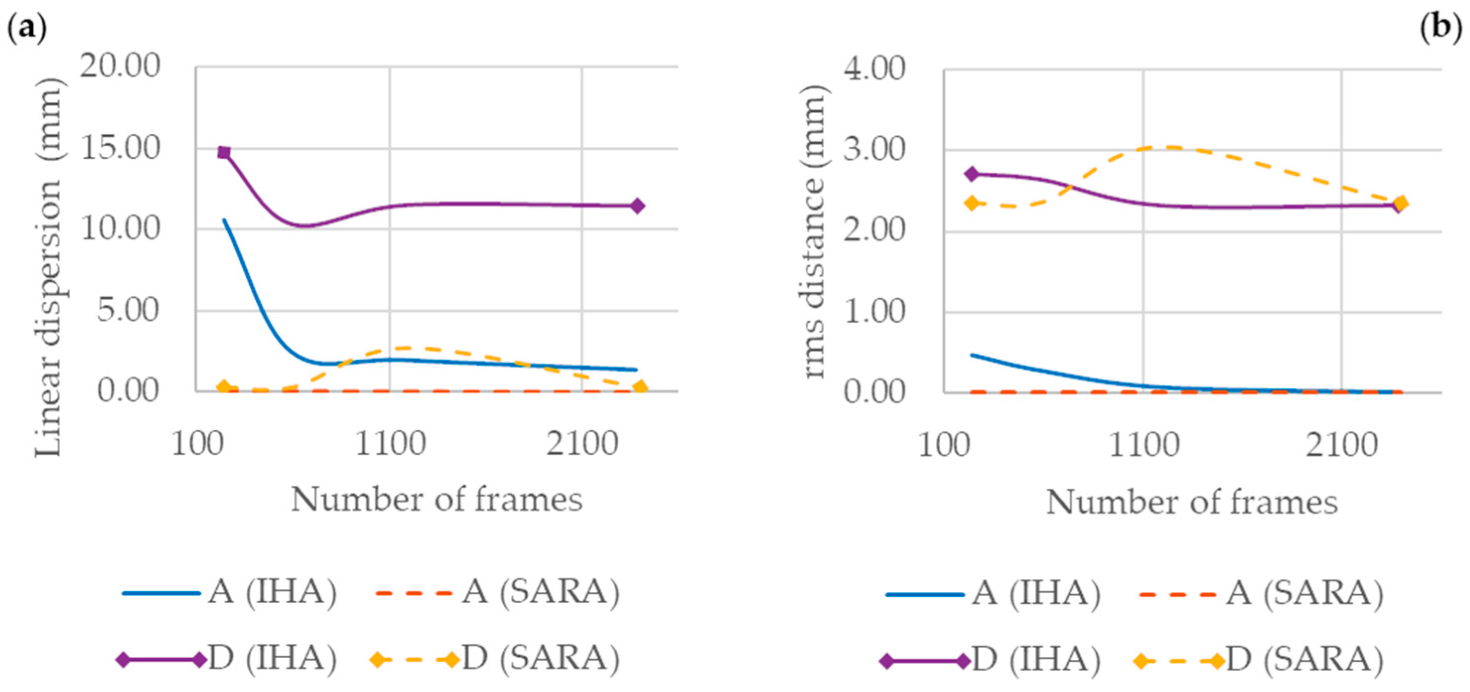
3.3. Results of S3 Set: Speed of Motion Patterns and Sampling Frequency

The dispersion parameters and the rms distance values resulting from the analysis, for the different speed and sampling frequency values selected, are presented in Appendix A,

Table A3. Dispersion parameters (d_eff, in mm, and χ_eff, in deg) and rms distance (Δ, in mm) between exact and estimated AoRs for different speeds and sampling frequency, in Hz, tested. Results are given for A and D motion configurations; the selected speed values (V1…V3) are detailed in Section 2.3.4. For each algorithm, the resulting number of time frames N_f is reported.

Conf.	Trial		IHA (w.1)				IHA (w.2)				IHA (w.3)				SARA
	V	fS	Nf	deff	χeff	Δ	Nf	deff	χeff	Δ	Nf	deff	χeff	Δ	Nf	deff	χeff	Δ
A	V1	100	463	1.96	1.64	0.07	463	1.96	0.49	0.13	463	1.97	0.17	0.25	480	0.03	0.02	0.01
	V1	250	1160	1.42	1.38	0.08	1160	1.42	0.42	0.07	1160	1.43	0.16	0.13	1200	0.04	0.02	0.01
	V1	500	2318	1.10	0.15	0.02	2318	1.10	0.05	0.05	2318	1.10	0.02	0.11	2400	0.04	0.02	0.01
	V1	1000	4633	0.80	0.12	0.02	4633	0.80	0.03	0.05	4633	0.80	0.01	0.08	4800	0.04	0.02	0.01
	V2	100	354	1.96	0.94	0.01	354	1.96	0.27	0.11	354	1.97	0.10	0.24	360	0.04	0.02	0.01
	V2	250	887	1.55	0.47	0.04	887	1.55	0.14	0.11	887	1.57	0.05	0.21	900	0.03	0.02	0.01
	V2	500	1769	1.62	0.14	0.06	1769	1.62	0.03	0.08	1769	1.64	0.01	0.15	1800	0.03	0.02	0.01
	V2	1000	3540	1.03	0.26	0.06	3540	1.03	0.07	0.06	3540	1.04	0.02	0.08	3600	0.03	0.02	0.01
	V3	100	240	10.6	0.17	0.47	240	10.7	0.06	0.39	240	11.1	0.02	1.48	240	0.03	0.02	0.01
	V3	250	591	2.46	0.46	0.28	591	2.50	0.16	0.62	591	2.67	0.07	1.14	600	0.03	0.02	0.01
	V3	500	1194	1.95	0.30	0.08	1194	1.95	0.08	0.12	1194	1.96	0.03	0.17	1200	0.03	0.02	0.01
	V3	1000	2383	1.35	0.02	0.02	2383	1.35	0.01	0.05	2383	1.36	0.00	0.12	2400	0.03	0.01	0.01
D	V1	100	463	11.1	3.60	2.34	463	11.1	1.42	2.32	463	11.1	0.58	2.41	480	0.30	0.27	2.35
	V1	250	1162	11.1	3.27	2.31	1162	11.1	1.30	2.28	1162	11.1	0.53	2.34	1200	0.31	0.27	2.63
	V1	500	2319	11.2	3.28	2.32	2319	11.2	1.31	2.30	2319	11.2	0.54	2.37	2400	0.30	0.27	2.51
	V1	1000	4637	11.2	3.27	2.33	4637	11.2	1.31	2.32	4637	11.2	0.54	2.41	4800	0.30	0.27	2.35
	V2	100	354	11.3	3.29	2.30	354	11.3	1.30	2.28	354	11.3	0.52	2.35	360	1.21	0.26	2.38
	V2	250	887	11.2	3.35	2.33	887	11.2	1.35	2.30	887	11.2	0.56	2.37	900	0.29	0.27	2.34
	V2	500	1771	11.3	3.31	2.32	1771	11.3	1.32	2.30	1771	11.3	0.54	2.39	1800	0.31	0.26	2.35
	V2	1000	3541	11.3	3.35	2.32	3541	11.3	1.34	2.31	3541	11.3	0.55	2.39	3600	0.29	0.26	2.36
	V3	100	240	14.7	4.42	2.70	240	14.7	1.92	2.92	240	14.8	0.86	3.46	240	0.29	0.25	2.35
	V3	250	591	10.3	4.52	2.63	591	10.3	1.96	2.85	591	10.4	0.87	3.24	600	0.30	0.26	2.36
	V3	500	1194	11.5	3.35	2.32	1194	11.5	1.34	2.29	1194	11.5	0.55	2.35	1200	2.67	0.26	3.04
	V3	1000	2385	11.5	3.35	2.32	2385	11.5	1.35	2.30	2385	11.5	0.56	2.37	2400	0.28	0.26	2.35

. The number of frames (N_f) considered by each algorithm is also presented.

When the lowest (V1) and average (V2) speed are considered, a limited improvement in the estimation of AoR positioning is observed by rising the sampling frequency for configuration A, whereas no significant improvement is shown for configuration D. In particular, for the 1-DoF motion configuration, the linear dispersion and rms distance are halved at 1000 Hz (about 1 mm), while the angular dispersion falls below 0.3 deg (starting from 0.9–1.64 deg at 100 Hz).

At highest speed (V3), the improvement in linear dispersion and rms distance obtained at a high sampling rate is evident for both motion configurations, although it is very clear especially for configuration A. The linear dispersion obtained at 100 Hz (10.6 mm) is reduced to 2.46 mm at 250 Hz, and it falls below 2 mm at higher frequencies. Similarly, the angular dispersion is generally reduced and achieves a very low magnitude (below 0.1 deg) at maximum frequency. The same behavior is observed for configuration D; however, the improvement in estimation accuracy is less significant.

The AoR estimation based on the SARA method shows an almost constant level of accuracy for most of the trials analyzed, which is generally higher than the one observed for the IHA approach. Figure 7 shows the estimation of the angular velocity performed by the IHA algorithm and its comparison with the angular velocity set as input of the multi-body model, by choosing motion configuration A. As shown in Figure 7a, the evaluation accuracy of the angular velocity at low speed (V1) is very high, as the AoR estimation. Figure 7b shows the same signals when a higher speed (V3) is selected. In this condition, by assuming a constant sampling rate, the angular velocity is predicted with less accuracy as compared to the result shown in Figure 7a. This outcome affects the accuracy of AoR estimation performed by means of the helical axis approach, whereas it has no impact on SARA methodology.

3.4. Results of S4 Set: Common and Random Sources of Additive Noise on Markers’ Trajectories

In Appendix A,

Table A4. Dispersion parameters (d_eff, in mm, and χ_eff, in deg) and rms distance (Δ, in mm) between exact and estimated AoRs for different common (SNR_cmn) and random (SNR_rnd) signal-to-noise ratios (in dB) of the corresponding sources of noise signals. Results are given for A and D motion configurations.

Conf.	Trial		IHA (w.1)			IHA (w.2)			IHA (w.3)			SARA
	SNRcmn	SNRrnd	deff	χeff	Δ	deff	χeff	Δ	deff	χeff	Δ	deff	χeff	Δ
A	100	100	1.91	1.30	0.10	1.91	0.35	0.06	1.95	0.11	0.14	0.02	0.01	0.01
	100	90	3.87	3.71	0.24	3.88	0.98	0.20	3.89	0.32	0.33	0.07	0.05	0.02
	100	80	8.04	10.0	1.37	8.06	2.76	0.83	8.10	0.97	0.55	0.21	0.16	0.08
	100	70	14.5	7.69	0.88	14.5	2.11	0.83	14.6	0.77	1.11	0.62	0.49	0.55
	90	100	14.7	7.69	0.83	14.7	2.11	0.67	14.7	0.77	0.98	0.62	0.49	0.55
	90	90	19.4	25.0	6.10	19.4	7.57	5.29	19.5	2.92	3.92	0.63	0.49	0.52
	90	80	25.6	29.2	15.1	25.6	8.88	15.8	25.7	3.41	15.9	0.66	0.53	0.54
	90	70	30.1	10.8	3.52	30.1	3.52	3.77	30.1	1.43	3.36	0.89	0.71	1.08
	80	100	32.7	10.8	3.78	32.7	3.52	4.10	32.8	1.43	3.83	0.90	0.71	1.07
	80	90	31.9	10.8	3.56	31.9	3.50	4.00	31.9	1.43	3.81	0.93	0.71	1.01
	80	80	32.2	26.6	22.4	32.2	8.14	22.6	32.2	3.14	23.5	0.98	0.72	1.10
	80	70	32.5	37.4	21.8	32.6	11.1	19.5	32.7	4.23	18.7	1.19	0.86	1.71
	70	100	53.1	37.4	21.9	53.1	11.1	20.3	53.1	4.23	20.1	1.32	0.86	1.74
	70	90	31.7	37.5	23.9	31.8	11.1	22.3	31.9	4.26	22.1	1.45	0.85	1.74
	70	80	35.7	36.1	22.0	35.8	10.9	21.1	36.5	4.15	21.1	1.59	0.86	1.59
	70	70	32.3	35.3	12.7	32.4	10.8	14.3	32.9	4.15	15.9	1.82	0.98	2.16
D	100	100	11.1	3.32	2.36	11.1	1.30	2.33	11.1	0.52	2.40	0.30	0.27	2.40
	100	90	11.4	3.56	2.31	11.4	1.38	2.25	11.4	0.55	2.26	0.31	0.27	2.42
	100	80	14.6	8.32	2.83	14.6	3.11	2.74	14.6	1.21	2.65	0.38	0.31	2.60
	100	70	24.9	15.0	4.73	24.9	5.56	4.32	25.0	2.18	3.83	0.77	0.55	2.36
	90	100	25.1	15.8	5.69	25.1	5.84	5.17	25.1	2.28	4.54	0.77	0.55	2.38
	90	90	24.9	15.6	5.40	24.9	5.77	4.91	25.0	2.26	4.30	0.82	0.55	7.01
	90	80	24.9	12.7	2.92	24.9	4.66	2.67	25.0	1.79	2.40	0.81	0.58	2.40
	90	70	23.6	28.9	7.67	23.6	10.5	6.95	23.7	4.15	6.27	1.07	0.73	2.51
	80	100	26.0	28.9	10.2	26.0	10.5	9.36	26.1	4.15	8.62	1.06	0.73	2.49
	80	90	24.1	28.6	8.23	24.1	10.3	7.47	24.2	4.06	6.67	1.07	0.73	2.15
	80	80	23.8	29.1	8.32	23.8	10.5	7.67	23.9	4.14	6.95	1.12	0.75	2.17
	80	70	28.1	31.7	11.7	28.1	11.3	11.0	28.3	4.43	10.0	1.28	0.85	2.15
	70	100	32.6	31.7	19.3	32.6	11.3	17.6	33.0	4.43	14.9	1.42	0.85	2.29
	70	90	29.0	31.6	9.52	29.0	11.3	9.04	29.1	4.40	8.52	1.53	0.86	2.19
	70	80	30.2	31.2	8.86	30.2	11.2	8.45	30.3	4.37	8.04	1.64	0.87	2.18
	70	70	35.3	13.7	2.94	35.3	5.01	3.63	35.3	1.94	4.49	1.89	1.00	2.48

, the dispersion parameters and the rms distance resulting from the analysis are collected for different combinations of common and random noise signals added to the markers’ trajectories provided by the multi-body model. Figure 8 and Figure 9 show a direct comparison between the MHAs obtained with the different weighting factors and the functional axes calculated with the SARA algorithm, respectively, for motion configurations A and D. The exact AoR is also shown to ease the interpretation of the results. All the plots refer to the shank LCS.

The results highlight the significant impact of marker noise on the accuracy of AoR estimated by helical axis methodology. This effect seems to be particularly highlighted in the transition between SNR_cmn = 100 dB and SNR_cmn = 90 dB, and it increases at low SNR_rnd values. For SNR_cmn values lower than 90 dB, the addition of a random noise signal does not seem to increase the linear dispersion of the IHA sets in a significant way. The same behavior is highlighted both in A and D motion configurations. On the other hand, the angular dispersion is generally increased by lowering the SNRs of both source signals, and this effect is even more relevant for configuration A. Surprisingly, although linear and angular dispersion parameters show a significant increase even at relatively low levels of noise, the accuracy of AoR estimation by means of the MHA is generally not compromised for SNR_cmn higher than 80 dB, regardless of the SNR_rnd values selected. This effect is more evident for configuration A as compared to the tri-planar motion configuration (D).

By comparing the results presented so far with the outcomes of the SARA approach, the latter clearly outperforms the helical axis methodology for all the noise conditions tested (see Figure 8 and Figure 9). In particular, the rms distance between the exact and estimated AoRs remains at very low values (below 5 mm) for almost all the trials, whereas it reaches about 20 mm (in the worst scenario) when the helical axis method is used. Figure 10 shows the estimation of the angular velocity performed by the IHA algorithm and its comparison with the angular velocity set as input of the multi-body model by choosing motion configuration A and different SNR_cmn values. A progressively worse evaluation of the angular velocity is obtained by increasing the SNR of the common noise signal, affecting the accuracy of the estimation algorithm.

4. Discussion

This paper proposed a comparison between the helical axis and SARA approaches for the estimation of functional joint axes, starting from simulated motion capture data provided by the multi-body modeling approach. Compared to similar studies from the literature that considered simulated motion data [26], the multi-body model provided additional flexibility to the configuration of the motion patterns, thus allowing an extended comparison between the performance of the two methodologies considered. In particular, this work provided a quantitative analysis in terms of dispersion and estimation accuracy of the functional joint axes estimated by the two algorithms that can improve the knowledge of the algorithms themselves, in support to other studies that compared the methods by a mathematical perspective [34]. Moreover, the effect of the different weighting factors in MHA estimation has not really been discussed by objective evaluation of the results, as presented in the current work. Reichl et al. [40] presented a comparison between finite helical axis and SARA on simulated motion data; however, they focused on a simpler knee joint model based on a compound hinge joint with 2 DoFs and did not provide any discussion about marker positioning, speed of motion patterns, and sampling rate. A similar analysis was conducted by the authors on experimental data [35]; however, this approach lacks the possibility to change the conditions of the trials with the same flexibility shown in the current paper.

4.1. AoR Estimation by Means of Helical Axis Is Significantly Affected by Time Discretization

As reported in Section 3.1, by varying the range and speed of motion patterns, a significant dependency between estimation accuracy and the number of time frames available was observed for the IHA algorithm. In particular, this phenomenon was highlighted when high speed and range of motion are considered. Indeed, given the constant sampling rate of the simulated motion capture data, those conditions correspond to the worst time discretization of the trajectories used to reconstruct joint motion. As confirmed by the simulations presented in Section 3.3, the improvement in IHA estimation accuracy, when higher than 100 Hz sampling frequencies are selected, is obvious, as signaled by the low values of linear dispersion d_eff and rms distance Δ achieved (Table A3). Of course, high sampling frequency values such as 1000 Hz are not desirable during real experimentation due to the limitations of the instrumentation and data acquisition systems, though significant improvements in estimation accuracy are shown even for more feasible solutions, such as 250 and 500 Hz. Moreover, high discretization would result in a large number of time frames that can affect the efficiency of the algorithms in applications where the computational time is relevant. As shown in Section 3.3, the SARA approach does not seem to be significantly influenced by the number of time frames, regardless of the speed selected. This result is quite interesting and widens the field of application of this methodology to fast and wide motion patterns, even for relatively low sampling frequency. The dependency between AoR estimation accuracy, in terms of linear dispersion, and time discretization of the motion patterns is highlighted by the results shown in Figure 11a and Figure 12a for representative conditions.

The results presented in Section 3.1 show that, when the linear dispersion of the IHA set is high, mainly due to large ROMs and speed, the rms distance is also increased (see Figure 11b and Figure 12b). This result signals that, in general, an increase in the linear dispersion has an impact on the estimation accuracy of the MHA position, regardless of the weighting factor chosen. As far as the angular dispersion χ_eff is concerned, it seems to be independent of the several ROM/speed combinations tested, but it is affected far more significantly by the weight selected for MHA estimation. In particular, the correction proposed by Ehrig et al. [34] shows the most limited angular dispersion among the several solutions, but it has an impact on the accuracy of AoR estimation in terms of its positioning (see Table A1, IHA (w.3) columns). The corresponding increase in rms distance was highlighted especially for motion configurations A (1 DoF, flexion/extension) and C (2 DoFs, helical motion), whereas it was quite negligible for the other configurations that share linear translation DoF of the AoR along the antero-posterior direction. The presence of translational motion occurring in the sagittal plane might mix up the analysis and should be investigated in the future. However, the results obtained by choosing the different weighting factors do not clearly support the use of one weight rather than the other. In general, the corrections help in achieving a more confined set of helical axes; however, they may compromise the identification of the correct location of the AoR.

4.2. SARA Generally Provides Better Estimation Accuracy Due to Its Intrinsic Stability

Compared to the helical axis approach, SARA highlighted the best performance in terms of rms distance between the estimated AoR and the exact one, which is the parameter used to assess the accuracy of the AoR estimation. In particular, this result was confirmed for A, B, and C configurations for all the conditions tested, whereas both algorithms performed in a similar way for the tri-planar motion configuration (D, as shown in Figure 11b and Figure 12b). As far as the linear and angular dispersion parameters are concerned, SARA showed the lowest values in most of the conditions observed; however, this result was expected since it is directly connected to its formulation being quite different than the IHA’s. As presented in Section 2.2.2, SARA initially considers two separate LCSs, respectively integral with the shank and foot, to evaluate the relative motion between each segment and the fixed GCS. In this calculation, each AoR is considered stationary with respect to the corresponding segment. Then, the functional axis obtained at the end of the procedure is estimated as the average of the AoRs calculated for each segment. Compared to the SARA approach, the helical axis does not consider any of those hypotheses for determining the relative motion between two rigid segments, yet the additional freedom of this methodology plays a key role in the “stability” of the results. For this reason, the variability in the IHA sets is expected to be more pronounced than the one observed as the outcome of the SARA algorithm. This aspect must be taken into account when the two methods are compared. For tri-planar motion (see Table A1), the angular dispersion obtained for the IHA approach is quite a good approximation of the actual orientation variability of the joint AoR imposed by the model; however, this is not confirmed for all the ROM/speed tested. On the contrary, linear dispersion is always an overestimation of the actual linear variability of the joint AoR. This confirms the weakness of the helical axis approach in determining the correct positioning of the AoR, already highlighted in the literature [34].

4.3. SARA Is More Suitable Than IHA for Kinematic Analyses Based on Noisy Markers’ Trajectories

As pointed out in the literature [40], the intrinsic variability of the helical axis approach also affects its sensitivity to noise. As confirmed by the results presented in Section 3.4, in which different levels of additive noise were considered to alter the markers’ trajectories as provided by the multi-body model, the performance of the IHA algorithm considerably worsen when SNR_cmn values lower than 80 dB are selected. In particular, the AoR estimation accuracy seems to be mainly affected by the source of the common noise signal, which is used to simulate non-rigid deformations of the marker clusters such as the one related to the soft tissue artifact. Oddly, the rms distance measured at the maximum level of the common noise signal decreases while lowering SNR_rnd. This result might be due to the high level of random noise, which could contribute to the overall noise signal by subtracting to the common one. The SARA algorithm, on the other hand, can benefit from the lack of numerical differentiation and filtering that IHA methodology requires [34,37]; therefore, it might be more suitable for any application based on position-based rather than velocity-based datasets, such as those provided by motion capture analysis. Numerical differentiation can indeed intensify the effect of noise on marker coordinates and compromise the reconstruction of joint kinematics. In addition, unlike the IHA methodology, the SARA algorithm does not require the calculation of the foot DoFs relative to the shank LCS, thus removing the impact of the errors associated with coordinate transformations. In support of these considerations, the AoR estimation performed by the SARA algorithm was always more accurate than the one obtained by application of the IHA methodology, even for high levels of noise.

4.4. Different Scattering of the Marker Clusters Has a Limited Impact on AoR Estimation Accuracy

Finally, the simulations presented in Section 3.2, which considered different scattering of the marker clusters on the surface of each segment, showed that no significant dependency between dispersion parameters and marker disposition was observed for both algorithms. The larger variability in estimation accuracy was obtained for the 1-DoF motion configuration (A); however, it was not possible to derive a correlation with the marker scattering in each cluster. This aspect should be taken into account during experimentation since marker positioning has an impact on bone pose estimation, which could not be investigated with the modeling approach considered in this study.

4.5. Limitations

The main limitations of this work are represented by the approximations in the ankle joint motion patterns that were provided as input for the multi-body model. In particular, the three rotational DoFs of the bushing joint do not accurately match the actual physiological ones. Unlike the anatomical interpretation of joint axes (antero-posterior, longitudinal, medio-lateral), the modeling of the joint in the multi-body approach considers three mutually orthogonal axes. Moreover, the DoFs associated with any joint axes are independent by mathematical formulation of the bushing. This feature leads to a simplified representation of the joint DoFs, which result to be decoupled in the model, whereas they cannot be isolated in the real scenario. For these reasons, the simulated flexion/extension, adduction/abduction, and inversion/eversion motion patterns can only approximate the real joint DoFs and have limited meaning from the anatomical/physiological point of view. However, this approximation was considered reasonable for the aim of the current work, which focused on the objective evaluation of the helical axis and SARA techniques in a realistic scenario, rather than on the accurate representation of ankle joint motion through multi-body modeling. Moreover, this simplification greatly facilitates the formulation of the model.

5. Conclusions

This paper showed a comparison between different approaches for the estimation of functional joint axes. The work was conducted at a simulation level by developing a multi-body model resembling the lower limb of a subject, which was used to generate simulated motion capture data. The helical axis and SARA approaches were used to estimate the AoR of the simulated ankle joint for several motion patterns and testing conditions. The main conclusions are reported in the following:

• For the 1-DoF and 2-DoFs configurations, the SARA proves to be more accurate than the helical axis methodology, regardless of the different conditions considered;
• For the 6-DoFs configuration, the SARA outperforms the helical axis approach when a high level of noise is considered or when the number of samples used to discretize the gait cycle is limited;
• The IHA methodology allows a description of joint kinematics that is intrinsically less constrained than the one enabled by the SARA. This could be useful when a more detailed, time-dependent representation of joint kinematics is necessary.

References

1. Renggli, D.; Graf, C.; Tachatos, N.; Singh, N.; Meboldt, M.; Taylor, W.R.; Stieglitz, L.; Schmid Daners, M. Wearable Inertial Measurement Units for Assessing Gait in Real-World Environments. Front. Physiol. 2020, 11, 90. [Google Scholar] [CrossRef] [PubMed]
2. Cappozzo, A.; Dellacroce, U.; Leardini, A.; Chiari, L. Human Movement Analysis Using Stereophotogrammetry: Part 1: Theoretical Background. Gait Posture 2005, 21, 186–196. [Google Scholar] [CrossRef] [PubMed]
3. Chiari, L.; Croce, U.D.; Leardini, A.; Cappozzo, A. Human Movement Analysis Using Stereophotogrammetry: Part 2: Instrumental errors. Gait Posture 2005, 21, 197–211. [Google Scholar] [CrossRef] [PubMed]
4. Page, A.; De Rosario, H.; Mata, V.; Hoyos, J.V.; Porcar, R. Effect of Marker Cluster Design on the Accuracy of Human Movement Analysis Using Stereophotogrammetry. Med. Bio. Eng. Comput. 2006, 44, 1113–1119. [Google Scholar] [CrossRef] [PubMed]
5. Davis, R.B.; Õunpuu, S.; Tyburski, D.; Gage, J.R. A Gait Analysis Data Collection and Reduction Technique. Hum. Mov. Sci. 1991, 10, 575–587. [Google Scholar] [CrossRef]
6. Benedetti, M.; Catani, F.; Leardini, A.; Pignotti, E.; Giannini, S. Data Management in Gait Analysis for Clinical Applications. Clin. Biomech. 1998, 13, 204–215. [Google Scholar] [CrossRef]
7. Frigo, C.; Rabuffetti, M.; Kerrigan, D.C.; Deming, L.C.; Pedotti, A. Functionally Oriented and Clinically Feasible Quantitative Gait Analysis Method. Med. Biol. Eng. Comput. 1998, 36, 179–185. [Google Scholar] [CrossRef]
8. Leardini, A.; Sawacha, Z.; Paolini, G.; Ingrosso, S.; Nativo, R.; Benedetti, M.G. A New Anatomically Based Protocol for Gait Analysis in Children. Gait Posture 2007, 26, 560–571. [Google Scholar] [CrossRef]
9. Gao, F.; Carlton, W.; Kapp, S. Effects of Joint Alignment and Type on Mechanical Properties of Thermoplastic Articulated Ankle-Foot Orthosis. Prosthet. Orthot. Int. 2011, 35, 181–189. [Google Scholar] [CrossRef]
10. Ferraresi, C.; De Benedictis, C.; Franco, W.; Maffiodo, D.; Leardini, A. In-Vivo Analysis of Ankle Joint Movement for Patient-Specific Kinematic Characterization. Proc. Inst. Mech. Eng. H 2017, 231, 831–838. [Google Scholar] [CrossRef]
11. Ferraresi, C.; De Benedictis, C.; Maffiodo, D.; Franco, W.; Peluso, A.; Leardini, A. A Methodology for the Development of a Hinged Ankle-Foot Orthosis Compatible with Natural Joint Kinematics. Mech. Mach. Sci. 2019, 73, 93–102. [Google Scholar] [CrossRef]
12. Kobayashi, T.; Orendurff, M.S.; Hunt, G.; Gao, F.; LeCursi, N.; Lincoln, L.S.; Foreman, K.B. The Effects of Alignment of an Articulated Ankle-Foot Orthosis on Lower Limb Joint Kinematics and Kinetics during Gait in Individuals Post-Stroke. J. Biomech. 2019, 83, 57–64. [Google Scholar] [CrossRef] [PubMed]
13. Leardini, A.; Aquila, A.; Caravaggi, P.; Ferraresi, C.; Giannini, S. Multi-Segment Foot Mobility in a Hinged Ankle-Foot Orthosis: The Effect of Rotation Axis Position. Gait Posture 2014, 40, 274–277. [Google Scholar] [CrossRef]
14. Leardini, A.; Chiari, L.; Croce, U.D.; Cappozzo, A. Human Movement Analysis Using Stereophotogrammetry: Part 3. Soft tissue artifact assessment and compensation. Gait Posture 2005, 21, 212–225. [Google Scholar] [CrossRef] [PubMed]
15. Bonci, T.; Camomilla, V.; Dumas, R.; Chèze, L.; Cappozzo, A. Rigid and Non-Rigid Geometrical Transformations of a Marker-Cluster and Their Impact on Bone-Pose Estimation. J. Biomech. 2015, 48, 4166–4172. [Google Scholar] [CrossRef]
16. De Rosario, H.; Page, Á.; Besa, A. Analytical Study of the Effects of Soft Tissue Artefacts on Functional Techniques to Define Axes of Rotation. J. Biomech. 2017, 62, 60–67. [Google Scholar] [CrossRef]
17. Manal, K.; Davis, I.M.; Galinat, B.; Stanhope, S. The Accuracy of Estimating Proximal Tibial Translation during Natural Cadence Walking: Bone vs. Skin Mounted Targets. Clin. Biomech. 2003, 18, 126–131. [Google Scholar] [CrossRef]
18. Benoit, D.L.; Andersen, M.S.; Damsgaard, M.; Ramsey, D.K.; Rasmussen, J. A Model to Compensate for Soft Tissue Artifact during Gait. Gait Posture 2009, 30, S5. [Google Scholar] [CrossRef]
19. Ferraresi, C.; De Benedictis, C.; Bono, L.; Del Gaudio, F.; Ferrara, L.; Masiello, F.; Franco, W.; Maffiodo, D.; Leardini, A. A Methodology for the Customization of Hinged Ankle-Foot Orthoses Based on in Vivo Helical Axis Calculation with 3D Printed Rigid Shells. Proc. Inst. Mech. Eng. H 2021, 235, 367–377. [Google Scholar] [CrossRef]
20. Gastaldi, L.; Lisco, G.; Pastorelli, S. Evaluation of Functional Methods for Human Movement Modelling. Acta Bioeng. Biomech. 2015, 17, 31–38. [Google Scholar] [CrossRef]
21. Monnet, T.; Desailly, E.; Begon, M.; Vallée, C.; Lacouture, P. Comparison of the SCoRE and HA Methods for Locating in Vivo the Glenohumeral Joint Centre. J. Biomech. 2007, 40, 3487–3492. [Google Scholar] [CrossRef] [PubMed]
22. Galetto, M.; Gastaldi, L.; Lisco, G.; Mastrogiacomo, L.; Pastorelli, S. Accuracy Evaluation of a New Stereophotogrammetry-Based Functional Method for Joint Kinematic Analysis in Biomechanics. Proc. Inst. Mech. Eng. H 2014, 228, 1183–1192. [Google Scholar] [CrossRef] [PubMed]
23. Woltring, H.J.; Huiskes, R.; de Lange, A.; Veldpaus, F.E. Finite Centroid and Helical Axis Estimation from Noisy Landmark Measurements in the Study of Human Joint Kinematics. J. Biomech. 1985, 18, 379–389. [Google Scholar] [CrossRef]
24. Woltring, H.J. Estimation of the Trajectory of the Instantaneous Centre of Rotation in Planar Biokinematics. J. Biomech. 1990, 23, 1273–1274. [Google Scholar] [CrossRef]
25. Chèze, L.; Fregly, B.J.; Dimnet, J. Determination of Joint Functional Axes from Noisy Marker Data Using the Finite Helical Axis. Hum. Mov. Sci. 1998, 17, 1–15. [Google Scholar] [CrossRef]
26. Ehrig, R.M.; Taylor, W.R.; Duda, G.N.; Heller, M.O. A Survey of Formal Methods for Determining Functional Joint Axes. J. Biomech. 2007, 40, 2150–2157. [Google Scholar] [CrossRef]
27. Leardini, A.; O’Connor, J.J.; Catani, F.; Giannini, S. Kinematics of the Human Ankle Complex in Passive Flexion; a Single Degree of Freedom System. J. Biomech. 1999, 32, 111–118. [Google Scholar] [CrossRef]
28. Leardini, A.; Stagni, R.; O’Connor, J.J. Mobility of the Subtalar Joint in the Intact Ankle Complex. J. Biomech. 2001, 34, 805–809. [Google Scholar] [CrossRef]
29. Lewis, G.S.; Sommer, H.J.; Piazza, S.J. In Vitro Assessment of a Motion-Based Optimization Method for Locating the Talocrural and Subtalar Joint Axes. J. Biomech. Eng. 2006, 128, 596–603. [Google Scholar] [CrossRef]
30. Sheehan, F.T. The Instantaneous Helical Axis of the Subtalar and Talocrural Joints: A Non-Invasive in Vivo Dynamic Study. J. Foot Ankle Res. 2010, 3, 13. [Google Scholar] [CrossRef] [Green Version]
31. Ehrig, R.M.; Taylor, W.R.; Duda, G.N.; Heller, M.O. A Survey of Formal Methods for Determining the Centre of Rotation of Ball Joints. J. Biomech. 2006, 39, 2798–2809. [Google Scholar] [CrossRef] [PubMed]
32. Camomilla, V.; Cereatti, A.; Vannozzi, G.; Cappozzo, A. An Optimized Protocol for Hip Joint Centre Determination Using the Functional Method. J. Biomech. 2006, 39, 1096–1106. [Google Scholar] [CrossRef] [PubMed]
33. Asadi Nikooyan, A.; van der Helm, F.C.T.; Westerhoff, P.; Graichen, F.; Bergmann, G.; (Dirkjan) Veeger, H.E.J. Comparison of Two Methods for In Vivo Estimation of the Glenohumeral Joint Rotation Center (GH-JRC) of the Patients with Shoulder Hemiarthroplasty. PLoS ONE 2011, 6, e18488. [Google Scholar] [CrossRef] [PubMed] [Green Version]
34. Ehrig, R.M.; Heller, M.O. On Intrinsic Equivalences of the Finite Helical Axis, the Instantaneous Helical Axis, and the SARA Approach. A Mathematical Perspective. J. Biomech. 2019, 84, 4–10. [Google Scholar] [CrossRef] [PubMed]
35. Reichl, I.; Ongaro, M. Finite Helical Axis versus Symmetrical Axis of Rotation Approach for the Human Knee Joint: Squats, Rowing and Cycling. Comput. Methods Biomech. Biomed. Eng. 2013, 16, 109–111. [Google Scholar] [CrossRef] [PubMed]
36. Colle, F.; Lopomo, N.; Visani, A.; Zaffagnini, S.; Marcacci, M. Comparison of Three Formal Methods Used to Estimate the Functional Axis of Rotation: An Extensive in-Vivo Analysis Performed on the Knee Joint. Comput. Methods Biomech. Biomed. Eng. 2016, 19, 484–492. [Google Scholar] [CrossRef]
37. Cappello, A.; La Palombara, P.F.; Leardini, A. Optimization and Smoothing Techniques in Movement Analysis. Int. J. Bio-Med. Comput. 1996, 41, 137–151. [Google Scholar] [CrossRef]
38. Berme, N.; Cappozzo, A. Biomechanics of Human Movement: Applications in Rehabilitation, Sports and Ergonomics; Bertec Corporation: Worthington, OH, USA, 1990; pp. 203–231. [Google Scholar]
39. Stokdijk, M.; Meskers, C.G.M.; Veeger, H.E.J.; de Boer, Y.A.; Rozing, P.M. Determination of the Optimal Elbow Axis for Evaluation of Placement of Prostheses. Clin. Biomech. 1999, 14, 177–184. [Google Scholar] [CrossRef]
40. Reichl, I.; Auzinger, W. Identifying Tibio-Femoral Joint Kinematics: Individual Adjustment versus Numerical Robustness. IFAC Proc. Vol. 2012, 45, 819–824. [Google Scholar] [CrossRef] [Green Version]
Figure 1. The methodology for the generation of noisy marker trajectories: (a) two views of the multi-body model, with markers on the shank (red) and foot (blue) highlighted, as well as the joint reference frame at the ankle (cyan); (b) the angular motion of the knee and ankle joints; (c) the linear motion of the ankle AoR; (d) downsampled and noisy marker trajectories in the global coordinate system. The plots refer to a generic tri-planar (6 DoFs) motion configuration.
Applsci 12 01274 g001
Figure 2. Random (red) and common (black) noise signals for different signal-to-noise ratios.
Applsci 12 01274 g002
Figure 4. IHA (yellow lines) and MHA (black dashed line) estimation for different motion configurations: (a) 1 DoF, flexion/extension; (b) 2 DoFs, flexion/extension + horizontal displacement; (c) 2 DoFs, helical motion; (d) 6 DoFs, tri-planar motion. Linear (in mm) and angular (in deg) dispersion parameters are reported in each plot. Lateral and medial tips of the exact AoR are represented in red and blue colors, green points are the intersection of the IHAs with two quasi-sagittal planes orthogonal to v axis and located at ±50 mm from the origin of the shank LCS.
Applsci 12 01274 g004
Figure 5. AoRs calculated with MHA, by choosing different weighting factors, and SARA, for motion configuration A. Each row and column correspond to a particular range of motion (ROM) and speed (V) selected, using the same nomenclature detailed in Section 2.3.2. The exact AoR imposed by joint kinematics setup is highlighted in dashed black line. All axes units are in mm.
Applsci 12 01274 g005
Figure 6. AoRs calculated with MHA, by choosing different weighting factors, and SARA, for motion configuration D. The axes are represented in two views: (a) transverse (horizontal) plane; (b) frontal plane. Each row and column correspond to a particular range of motion (ROM) and speed (V) selected, using the same nomenclature detailed in Section 2.3.2. The exact AoR imposed by joint kinematics setup is highlighted in dashed black line. All axes units are in mm.
Applsci 12 01274 g006
Figure 7. The absolute value of the angular velocity signal, as imposed by the model (ωAnkle, dashed line) in motion configuration A, and as estimated by the IHA algorithm (ωIHA). The two plots were obtained by considering the same sampling frequency (fS = 100 Hz) and different motion speed: (a) lowest speed, V1; (b) highest speed, V3. Dispersion parameters are reported in each plot.
Applsci 12 01274 g007
Figure 8. AoRs calculated with MHA, by choosing different weighting factors, and SARA, for motion configuration A. Each row and column correspond to a particular level of common and random noise signals, in terms of signal-to-noise ratios. The exact AoR imposed by joint kinematics setup is highlighted in dashed black line. All axes units are in mm.
Applsci 12 01274 g008
Figure 9. AoRs calculated with MHA, by choosing different weighting factors, and SARA, for motion configuration D. Each row and column correspond to a particular level of common and random noise signals, in terms of signal-to-noise ratios. The exact AoR imposed by joint kinematics setup is highlighted in dashed black line. All axes units are in mm.
Applsci 12 01274 g009
Figure 10. The absolute value of the angular velocity signal, as imposed by the model (ωAnkle, dashed line) in motion configuration A, and as estimated by the IHA algorithm (ωIHA). The plots were obtained by considering SNRrnd = 100 dB, and different levels of common noise signal: (a) SNRcmn = 100 dB; (b) SNRcmn = 90 dB; (c) SNRcmn = 80 dB; (d) SNRcmn = 70 dB.
Applsci 12 01274 g010
Figure 11. Linear dispersion (a) and rms distance (b) in A and D motion configurations, for different number of frames, obtained by increasing the joint motion speed. Results are shown for IHA (w.1) and SARA algorithms.
Applsci 12 01274 g011
Figure 12. Linear dispersion (a) and rms distance (b) in A and D motion configurations, for different sampling rate. Results are shown for IHA (w.1) and SARA algorithms.
Applsci 12 01274 g012