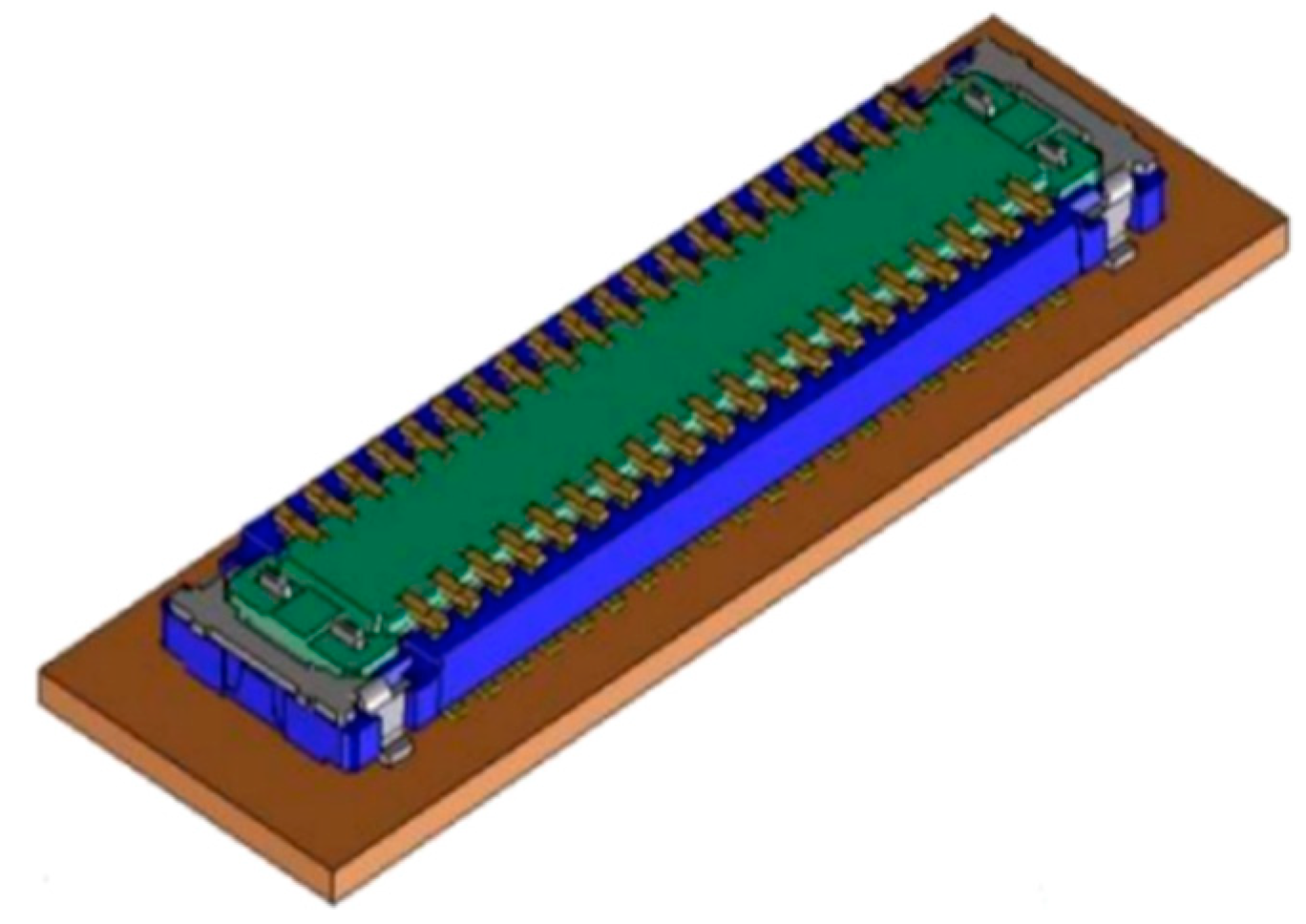
Article

Study on Data-Driven Approaches for the Automated Assembly of Board-to-Board Connectors

College of Mechanical and Electrical Engineering, Graduate Institute of Automation Technology, National Taipei University of Technology, Taipei 10608, Taiwan
*
Author to whom correspondence should be addressed.
Appl. Sci. 2022, 12(3), 1216; https://doi.org/10.3390/app12031216
Submission received: 8 November 2021 / Revised: 10 January 2022 / Accepted: 17 January 2022 / Published: 24 January 2022
(This article belongs to the Topic Artificial Intelligence in Sensors)

Abstract

:
The mating of the board-to-board (BtB) connector is rugged because of its design complexity, small pitch (0.4 mm), and susceptibility to damage. Currently, the assembly task of BtB connectors is performed manually because of these factors. A high chance of damage to the connectors can also occur during the mating process. Thus, it is essential to automate the assembly process to ensure its safety and reliability during the mating process. Commonly, the mating procedure adopts a model-based approach, including error recovery methods, owing to less design complexity and fewer pins with a high pitch. However, we propose a data-driven approach prediction for the mating process of the fine pitch 0.4 mm board-to-board connector utilizing a manipulator arm and force sensor. The data-driven approach uses force data for time series encoding methods such as recurrence plot (RP), Gramian matrix, k-nearest neighbor dynamic time warping (kNN-DTW), Markov transition field (MTF), and long short-term memory (LSTM) to compare each of the model prediction performances. The proposed method combines the RP model with the convolutional neural network (RP-CNN) to predict the force data. In the experiment, the proposed RP-CNN model used two final layers, SoftMax and L2-SVM, to compare with the other prediction models mentioned above. The output of the data-driven prediction is the coordinate alignment of the female board-to-board connector with the male board-to-board connector based on the value of force. Based on the experiment, the encoding approach, especially RP-CNN (L2-SVM), outperformed all prediction models as mentioned above with an accuracy of 86%.

1. Introduction

All devices utilize a PCB board to function and incorporate various electronic devices. One of these components is a board-to-board connector used to connect two wires or two circuits robustly. Figure 1 illustrates a surface-mounted board-to-board connector with 20 × 2 pins. Electric connectors use in various applications, such as mobile devices, tablets, and transportation [1]. Furthermore, experts assess the importance of automation in the assembly line in the industrial sector according to four main points: (1) increasing production rate, (2) enhancing production speed, (3) optimizing production, (4) assisting human tasks, and (5) improving cost-effectiveness.
Due to design complexity, fine pitch 0.4 mm board-to-board connectors are assembled manually in the production units. The industry’s most common challenges faced in the assembly line are aligning male and female pairs and fast-mating the connectors because of the complex design. In addition, performing the mating process without damage is one of the biggest challenges because humans cannot perceive the correct amount of force applied. Sometimes, this leads to a fault or damage to the pins in the connectors. In addition, the board-to-board connector assembly relies on a faintly audible clicking sound made by the connector during successful mating. However, it is not a reliable method to determine whether the process is a successful insertion. In addition to these challenges, there are various other constraints such as (1) the position of the male and female board-to-board connectors on the device, (2) obstacles surrounding the connector, (3) the size, and (4) the number of pins, as this increases the complexity of the mating process.
Due to the utilization of different types of connectors for other purposes and variations in design, these constraints may vary and affect the adopted method. The model-based approach has limitations due to the system’s complexity, tolerance range, and size. In addition, there is less research available that addresses the challenge of fine-pitch connector insertion. To the best of our knowledge, no study has been conducted on the fine pitch for the sole purpose of insertion position optimization. Considering these factors gives rise to a data-driven approach to overcoming the constraints above. Advancements in machine learning techniques have proved to be one of the best data analysis techniques. We can exploit these properties to make the mating process more reliable, efficient, and faster.
Due to the design complexity, as illustrated in Figure 2, the operation of board-to-board mating is performed manually in the industry. This is mainly because of the immense complexity and challenges in design and pitch size (0.4 mm). This research aims to determine an effective mating process by predicting the mating connector location based on the collected force data on the BtB mating using our proposed approach, which uses an encoding technique and CNN model for prediction.
Our proposed approach allows the user to analyze the collected force dataset, especially from the fine pitch BtB connector, which uses an industrial robot mounted with a force sensor. Here, the industrial robot performs designated motion on the BtB connector based on a defined trajectory. Then, we encode the collected force data into 2D image data to train the CNN model and 1D time series models to compare the model’s prediction performance. Based on this study, we can understand which model performs better in this application.

2. Existing Research

This section describes the existing research about the mating connector comprising technique and data analysis. Figure 3 illustrates the literature review mapping for the board-to-board connector as well as related topics, including (1) position error mitigation, (2) blind search strategies, and (3) vision force-guided system. These topics are strongly related to the mating process on the Peg-Hole Connector Insertion technique. In addition, the data analysis section discusses probabilistic, machine learning, and encoding approaches. For a quick overview of each existing research approach in this application, please see Table 1.

2.1. Peg-Hole Insertion Connector Technique

A general peg-hole is also a ubiquitous method that involves the analysis of force during the mating process. As in other insertion methods, a positioning error results in a reaction force between the surfaces, which causes some damage [2]. Various researchers have adopted different approaches to compensate for the reaction forces. Simultaneously, Daniel [3] presented the situation of jamming, absorbed between two surfaces by utilizing compliance devices to compensate for the reaction force and avoid damage. He used variable remote center compliance (VRCC), which had a shear pad of elastomers to alter the center of the compliance during the insertion, owing to the reaction force. Nagarajan [4] utilized remote center compliance (RCC) to compensate for the reaction force. The material also offered a greater force required to complete the insertion process. A few other research studies adopted the active method in the peg-hole approach by utilizing Gaussian mixture regression to copy the movement of a human hand in the lead by teaching and implementing a force control strategy for autonomous insertion [4]. In addition, Di [5] utilized the error recovery strategy from the size information of the connector and adjusted the compliance motion for successful mating of the four-pin plug-in connector.
The most common technique for peg-hole insertion is Blind Search. There are other blind search strategies, such as the spiral, probing, and binary trajectory techniques. The tilt strategy was selected in the peg-hole insertion when no visual system was available for assistance [6]. Due to its design, blind search strategies and passive method techniques have been widely applied to these macro systems. However, these techniques cannot be utilized directly at the micro-level, as there is a vast difference in the design of connectors. Connector mating has three categories: (1) arriving, (2) exploring, and (3) mating. Chen utilized a four-pin plug-in connector to analyze the assembly task and proposed four search algorithms based on force/moment data [7]. The four search algorithms are as follows: (1) spiral search, (2) probing search, (3) binary search I, and (4) binary search II. These algorithms indicated the relationship between the change in force based on the misalignment during insertion, followed by error recovery.
Huang and Song [8,9] proposed a hybrid vision-force-guided system for a four-pin plug-in connector. Di [5] stated a combination of vision and force on the fault inspection online. It improves the rate of detecting the system’s error and makes it more robust when utilizing the data provided by the force and vision system. First, the vision system takes an image as an ideal case, uses it as a benchmark, and compares the rest of the image with this benchmark image. It determines the change in coordination with both images and predicts the fault in grasping. Therefore, if the grasping is not straight, there will always be some error in insertion, owing to the small space available for insertion. It has an extra step in detecting the vision system’s connector for grasping. The tilting strategy combined with impedance control can overcome the position error caused by the vision system in the grasping procedure.
To overcome the challenge of [5], “iHand-designed” was explicitly utilized for connector grasping and achieved an insertion rate of 99 % [10]. This particular type of gripper helps predict the distance variation with the connector. It detects the deformation in the PCB. Fransico [11] designed a gripper for accurate alignment and for analyzing the permissible tolerance range of plug-in connectors. Franciso also [12] tested 70 plug-in connectors of various sizes and performed the mating process utilizing a robot arm and a robotic adaptive gripper. It provided the tolerance dataset solely for the plug-in connectors but not the fine pitch surface mount connector.

2.2. Data Analysis on Mating Connector

According to Chunghun [13], the probabilistic approach for the mating process indicates the connector’s analysis at different states and what a connector encounters during the process of mating. At the preliminary stage, it utilized the method from Kubota [14] that all the connectors produced visual, audible, and force signals during mating and used them for the analysis by using logistic regression. Jian [15] chose a fuzzy pattern match to detect and diagnose failures during the mating process. The speed also affects the mating operation, as the insertion rate directly influences the peak of the force in the mating process [16]. Approximately all research utilizes a plug-in connector with PINs varying between 4 and 8 pins.
Presently, reinforcement learning (RL) is also extensively discussed in the assembly system, especially the peg-in-hole (PIH) method. The PIH approach generally differs in search and insertion [17]. Hou [18] proposed fuzzy logic-driven variable time scale prediction-based reinforcement learning to improve the efficiency of a reinforcement learning algorithm in the PIH assembly process, which successfully decreases the assembly time by about 44% compared to the Deep-Q Learning approach [19]. Then, Gerrit [20] proposed meta-reinforcement learning to solve the PIH approach in five experiments, namely (1) straight downwards; (2) random search; (3) spiral search; (4) RL-PEARL from scratch; and (5) PEARL Sim2Real. The result indicated that their method could solve the PIH approach in less than 20 trials. Similarly, Sagar [21] initiated research on the PIH approach using generative adversarial imitation learning (GAIL) to help the robot learn within 20 episodes of human expert demonstration. The approach could improve the insertion time by five seconds compared to the standard operation.
In linear research about reinforcement learning, the study discusses the assembly process by imitating human behavior, still a hot topic in this field. Abbu-Dakka [22] solved the peg-in-hole task by human demonstration using exception strategies. Moreover, De Chambier and Suomalainen [23,24] proposed learning compliance for assembly motion demonstration. The key idea of these methods is to learn from human demonstration and exploration for the distribution in their dynamic model, as Dennis mentioned in his research [25].
As a result, the inspiration for using the encoding method of our data was inspired by Zhinguang and Martinez [26,27,28], which applied Gramian angular field (GAF) and Markov transition field (MTF) on the time series data. Furthermore, Hatami [29] tried to classify the time-series images using a deep convolutional neural network. However, in this study, we propose a data-driven approach method based on a fine pitch 0.4 mm connector with a 20 pin connector to predict the best location within a small area of insertion. Figure 2 illustrates a plug-in connector whose size is significantly more prominent with a simplified design than the standard BtB connector. The fine pitch BtB connector is an optimized interconnect solution for a smaller and thinner electronics product [30]. It originates for compact and high-density packaging electronics devices. The following section will explain each fundamental theory related to our research, including the various deep learning techniques utilized on our dataset for the prediction to assemble the board-to-board connector.

2.3. Novelty

The novelty of our approach is to predict the class data for the mating position using our encoding RP-CNN method compared to other models. The prediction aims to correctly predict the force class for the mating process on the board-to-board connector. The detailed approach of the proposed method will be described in the following section.

3. Materials and Methods

The research objective is to analyze the mating of the board-to-board connector utilizing a data-driven approach with a reliable prediction of the alignment of the connectors for safe and successful mating. This study used an articulated robotic arm for the mating process mounted with a force sensor and a suction cup as the gripper on the end-effector. Furthermore, the proposed method uses several encoding methods to transform the force data into graphical representative (2D Image). The outcome of the system is the prediction of which classes of forces are suitable for the mating process board-to-board connection.

3.1. Connector Overview

The connector utilized in this research is a fine-pitch board-to-board connector mainly used in mobile phones and tabs. It has a slight angle with a mating height of 0.80 mm with 25 pins on each row. Table 2 presents the specifications of the connector, while Figure 4 illustrates the pitch of the pin and the total width of the fine-pitch BtB connector.

3.2. Assumptions and Limitations

In this section, we discuss the constraints that affect connector mating. The board-to-board connector has certain limitations based on the manufacturing and position of the BtB on the device. Figure 5 illustrates that the X and Y movement is limited to 0.18 mm and 0.23 mm, respectively. This tolerance means that as long as the male BtB connector remains in the range of 0.23 mm in the Y and 0.18 mm in the X direction, the mating will always be successful. Therefore, this study was performed in a controlled environment, ensuring that the connector did not exceed the tolerance range area in any data collection process.
There was no extra bending in the PCB board, as the experiment was performed at a low speed [14]. The other factor based on the speed is the effect owing to the rate of assembly, which may involve extra force and sudden jerks, causing the force value to increase and damage it. Another assumption is that the entire movement is in the vertically downward direction, and the Z-axis of the force sensor is on the vertical axis. In this research, we analyzed the data of the Z-axis of the force sensor as the insertion mating was performed vertically downward by pushing the male connector in the female connector for mating. Thus, our research focuses on processing the collected force data using the encoding approach and predicting it using the CNN layer.
Since we needed to collect the force data first as our reference for the successful insertion, this research applies only to insertion applications with reference data (golden sample) to map the data first for the following mating process.

3.3. Preview of the Connector

In this experiment, the BtB connector has a significant limitation. The lower part contains a PCB board with a female BtB connector. The upper part of the device comprises a male connector attached to the device with the help of a flexible film. This flexible material allows the male BtB to move freely in the X and Y directions. Figure 6 illustrates the upper part of the device, and the area marked in red is the board-to-board connector. The shiny part is a connector underneath the board-to-board connector. Figure 7 illustrates the other side of the male board-to-board connector, as it shows two rows of pins with 25 pins on each side, as mentioned in the previous section.

3.4. Architecture

The physical system of the experiment comprises an articulated robot arm, a force sensor, and a suction cup on the end effector of the robot. In this section, we discuss the hardware, followed by the design of the entire physical system. The robot utilized is a Staubli TX 40 equipped with a DynPick Wacoh force sensor. Thus, it has been calibrated to compensate for the sensor’s extra weight. Figure 8 illustrates the system flowchart in which we utilize the TCP/IP to control the robot and the RS 232 protocol to collect the data from the force sensor. Figure 9 illustrates the overall flow of the system in the proposed study.

3.5. Dataset Collection

The robotic arms perform a downward push motion in the Z-direction with the suction cup mounted on the end effector, as shown in Figure 10. This suction cup sucks the plane metal outer surface of the board-to-board connector (as shown in Figure 6) and moves the projection accordingly. We experimented in a specially designed and controlled environment to collect the force data from the board-to-board connector mating process. When the movement is within the range of the limitation of the mating process (from 0.18 mm to 0.235 mm), the mating process will be successful.
Figure 11 shows the force data gathered from the mating operation. The G refers to the male connector’s position always staying aligned to the female connector.
The force data were collected in every 0.02 mm movement in the connector’s X–Y direction. Every displacement of the connector is marked with a number to represent the force data collected during the mating process. It also describes the distance from the G point, which is an initial point. We labeled the corresponding area of the BtB connector with four classes, as illustrated in Figure 11. The dataset would train the CNN model in the encoding method. Later on, the model can predict classes for the BtB insertion application.

3.6. Nature of the Data

This section describes the nature of the data from the collected force sensor data. Mainly it consists of record number, translational, and moment force data. Figure 12 represents the format data of the sensor. It also describes the primary axis sensitivity value as stated on the LSB/N unit.
Here, Figure 13 shows the collected data as (.csv) files. It contains the force sensor data, including the translational, moment, elapsed time, and record number. To convert the value to actual force data, we use the following Equation (1)
Figure 13. System diagram.
Applsci 12 01216 g013
D e t e c t e d   l o a d   [ N ] = ( d e t e c t e d   v a l u e   f r o m   s e n s o r [ L S B ] z e r o   p o i n t   o u t p u t   v a l u e   [ L S B ] ) m a i n   a x i s   s e n s i t i v i t y   [ L S B N m ]  
where,
  • detected value from sensor [LSB] = FX − MZ;
  • zero-point output value [LSB] = 8192 ± 655;
  • main axis sensitivity [LSB/Nm] = ±32.800, 32.815, 32.835, 1653.801,1634.816, 1636.136.
The robot moved downward in the Z direction with a pre-defined trajectory to push the plug into the receptor, as mentioned in Figure 11. As the robot’s performance dataset states, the robot’s minimum repeatability accuracy was ±0.02 mm, which was more significant than our minimum movement area. That aspect would affect the accuracy and precision of the force sensor’s measurement. Therefore, we designed classification experiments with four data classes to overcome this problem. The force information on a single point on the BtB shows that the force value varied in a range, as illustrated with the bar chart with an error in Figure 14. Based on this situation, we divided the connector area into four classes: first class, second class, third class, and fourth class.
The main parameters of the collected force data were coordinate location and the force itself. We tried to model the data based on the time-series model. A time series contained data points organized in time; hence we assigned the coordinate data to act as time. Figure 15 shows the illustration sample of the force data modeling as time-series data in a single coordinate point.

3.7. Deep Learning for Prediction

This section briefly discusses the various deep learning techniques utilized to test the datasets by predicting highly accurate classes. The details of the collected dataset from the previous section are available in Table 3 and Figure 16. As mentioned in Figure 9, our proposed method used the encoding data method to change the series data into a representative 2D image. The following section describes how the encoding method transforms the series force data into a representative 2D image.

3.7.1. Recurrence Plot

The recurrence plot is a technique utilized to analyze non-linear systems. It is mainly a visualization of recurrent states of the dynamic system. Technically, the recurrence plot helps us reveal all the times when the phase space trajectory of the dynamic system visits roughly the same area in the phase space. Here, we represent all the recurrence plot events as a mating process. The RP visualizes a two-dimensional square matrix. Matrix elements refer to the period in which a dynamic system repeats. In this matrix, both columns and rows correspond to a particular pair of times. This visualization technique indicates the recurrence of a specific state in a non-linear system. This visualization aims to inspect the various phase-space trajectories. The RP reveals small and large-scale patterns formed based on the relationship between the series on the row and column. If observed closely in the images of RP, it indicates single dots and diagonal lines accompanied by horizontal and vertical lines. The single dots in the RP suggest that the particular states are rare, whereas the horizontal lines and vertical lines indicate that a few of the conditions in the system are not altered, or the change is prolonged. The time-series analysis tasks usually comprise fitting the curve, estimating function, forecasting and prediction, classification, and clustering categories.
R i j = θ ( ϵ | | s i s j | | ) ,   s ( . )   ϵ   R ,   i ,   j = 1 ,   . K = 1 ,
where:
θ   Heaviside function
K   The number of considered states
s i ,   s j   The state-space
ϵ  Threshold distance
Equation (2) represents the recurrence-encoding Equation., which contains single dots, diagonal, vertical, and horizontal lines. The textures in the 2D image describe the relationship between the two states, where the fading indicates that the series contains a trend. Similarly, as discussed above, the horizontal and vertical lines indicate a tendency. However, these patterns are not easy to perceive directly with human eyes, as Silva [31] described the steps to calculate RP for a univariate time signal. A phase space trajectory and the RP matrix indicate various states’ closeness in the phase space. The threshold distance in Equation (2) represents the distance between the two states: Figure 17 illustrates the encoding method for the datasets.

3.7.2. Gramian Angular Summation Field (GASF)

We utilized our dataset to predict the Gramian angular summation field of the advanced algorithm on the UCR time-series classification dataset. The GASF technique Equation (3) encodes the 1-D data to a 2-D matrix as indicated in Equation (4). We encode 1-D data to the 2-D GASF matrix by utilizing the piecewise aggregate approximation (PAA) [32], which takes the mean of the back-to-back points of the 1-D data. Using the PAA technique on our dataset, we obtained a length of 25 without losing important data. Subsequently, the data are rescaled between (0, 1) to be fitted into the GASF matrix. Figure 18 displays the encoding method of the GASF, while Figure 19 illustrates the pipeline of the encoding method for GASF.
Figure 18. Gramian angular summation field (GASF) encoding in each class.
Applsci 12 01216 g018
c o s   ( φ i + φ j ) = X · X = 1 a r c c o s   ( c o s ( x i ) ) 2   ·   1 a r c c o s   ( c o s ( x j ) ) 2 c o s ( ϕ i + ϕ i ) = X · X ( ( I x 2 )   ·   I X 2 )
where,
X’—transpose of X
I—Identity Matrix
ϕ —when ϕ [ 0 , π ]
[ s i n   ( φ 1 + φ 1 ) s i n   ( φ 1 + φ 2 ) s i n   ( φ 2 + φ 1 ) s i n   ( φ 2 + φ 2 ) s i n   ( φ 1 + φ n ) s i n   ( φ 2 + φ n ) s i n   ( φ n + φ 1 )   s i n   ( φ n + φ 2 )     s i n   ( φ n + φ n ) ]  
Figure 19. Encoding method in each class.
Applsci 12 01216 g019

3.7.3. Gramian Angular Difference Field (GADF)

Figure 20 illustrates the encoding data for each class utilizing the Gramian angular difference field (GADF) technique. The GADF technique uses a piecewise aggregate to rescale the input data between (0, 1), and it comprises a kernel size of 2 × 2, followed by two max-pooling layers. The model implements three dropout layers of 0.2, 0.2, and 0.3 to ensure that the model is efficient. In the fully connected layer, the model utilized two dense layers with 128 neurons in both layers and the activation function ReLU, as illustrated in Figure 21.
Finally, the four neurons and the SoftMax function aim to predict the output layers on the available classes. Table 4 presents the final hyperparameters adopted after testing various properties and fine-tuning the network.

3.7.4. Markov Transition Field (MTF)

The Markov transition field (MTF) is another encoding technique utilized in this experiment. It represents the transition probability from one state-space to another and can predict the trend of the following data series. Also, it is a visualization technique to highlight the behavior of time-series data. We use this technique on our dataset to predict the position of the male BtB connector, as illustrated in Figure 9. Each time series has 50 values, so we encoded the values to MTF and obtained a 2D encoding of size (50 × 50) for each sequence in the dataset. Figure 22 illustrates the encoding result utilizing the MTF. The CNN network has three convolutional networks with ReLU and three max-pooling layers with kernel sizes of 3 × 3 and 2 × 2, respectively. The fully connected layers have three layers of 128, 135, 135, and four neurons. The model utilizes three dropouts of values (0.3), (0.4), and (0.2). We use the Adam optimizer with an initial value of 0.001 with an L2 regularizer to reduce overfitting in the model and train the model for 350 epochs. Table 5 shows the details of the adopted hyperparameters in the MTF CNN network.

3.7.5. K-Nearest Neighbor (kNN) Dynamic Time Warping (DTW)

The kNN DTW algorithm ensembles two methods, kNN and dynamic time warping. The most difficult challenge in utilizing kNN is determining the measures, i.e., the k value, which can accurately determine the similarity of the two data series [33]. It takes a warping distance parameter, which means how similar in the series it can be compared. We adopted k values of (3, 7, 9) and (11, 13, 15) to predict the classes. Hence, we chose these values based on the k value selection parameters while considering the warping distance. Table 6 lists the warping distance with the k values.

3.7.6. Long Short-Term Memory (LSTM)

We also tested our data utilizing the deep learning algorithm made for the series data. Here, we used LSTM for the sequence classification task. Figure 23 illustrates the architecture of the LSTM model designed for training our classification model. In our LSTM architecture, we used two LSTM layers with 50 cells. It has three dense layers with two dropouts (0.2, 0.2) between the dense layers. The output layer represents four neurons and the SoftMax activation function to predict the class.

4. Results

This section discusses the performance of various models in BtB applications. Firstly, we describe our performance using the encoding approach (RP, GAF, MTF) and demonstrate our result using the machine learning approach such as LSTM and kNN-DTW. The main reason for comparing these approaches is that our dataset acts as a time-series dataset.

4.1. Recurrence Plot

In this model, we utilized the recurrence plot encoding method to obtain a grayscale image and then the CNN model to train and predict the classes. We used two types of final layer: SoftMax and L2-SVM layers. For the SoftMax layer, we apply a cross-entropy as the loss function in ConvNet. In the L2-SVM, we tuned the network with two optimizers, SGD and ADAM.
Figure 24 (left) illustrates the accuracy graph of the model with the SoftMax layer, with a training accuracy of 86% and a test accuracy of 78%. Nonetheless, It also shows the loss of the model with the SoftMax layer with a cross-entropy optimizer. The model indicates a few signs of noise loss, meaning that the weight decay is not smooth. However, SoftMax utilizing cross-entropy achieves a lower error value because the cross-entropy uses the log to penalize each error. This penalty value depends on the value of the error. Therefore, the accuracy increases, leading to a minor penalty and helping the model achieve a lower error value.
Figure 24 (right) represents the confusion matrix of the SoftMax CNN model. The prediction of the classes is significantly high in the first and fourth classes. The generalization gap in the error values of testing and training affects the accuracy of the third class. Here, the error is lower in the SoftMax loss, but its optimization and weight decay are not as smooth as those of the L2-SVM with SGD. The L2-SVM utilizes a kernel-regularizer, also called the weight decay factor, with a value of 0.01 in the final output layer.
Figure 25 (left) illustrates the accuracy graph of the L2-SVM with SGD with 78% training. During testing, it reached 71% accuracy. The model shows the loss graph of the L2-SVM with SGD. It settles with less noise, but the loss value remains in the range of 0.9 to 0.8. One possible reason for this phenomenon is the low learning rate, which slows graph convergence. In addition, Figure 25 (right) illustrates the confusion matrix of the SGD-tuned RP model with L2-SVM. We utilized the squared-hinge loss as the loss function with the L2 kernel regularizer and the SGD optimizer. The squared hinge rapidly increases the error value by penalizing it quadratically. However, the SGD optimizer is slower than Adam; it converges slowly.
Nevertheless, Adam seems to be a challenge because of its fast convergence. Therefore, if the value of the learning rate (α) and beta1 (β1) is average or high, it will approach the convergence rapidly, jump the convergence point, and start overfitting. Hence, we utilized an early stopping technique to achieve the best convergence to avoid this issue. Figure 26 (left) shows the result of the RP model with L2-SVM, including model accuracy, model loss, and the confusion matrix.
Table 7 and Table 8 present the comparison table of all the SoftMax and L2-SVM accuracy values with the SGD and Adam CNN models.

4.2. Grammian Angular Field

We utilized the GASF encoding method on our dataset to train the CNN network for alignment prediction. The image we used was grayscale as the input for the CNN, and we applied the PAA technique to the sequence length in the preprocessing technique. Figure 27 illustrates the accuracy and loss graph of the GASF model. It offers 74% and 73% accuracy in training and testing, respectively. We utilized early stopping with a tolerance value of 40 epochs to ensure that the model did not reach overfitting. In addition, an L2 kernel regularizer in the second layer of the fully connected layer helped in weight decay and smoothly optimized the model with an initial value of 0.01. This method also produced a lower error rate of 0.53 and 0.61 for the training and test, which means the classification will be better in the classes. After applying the dropouts of 0.2 and 0.34, the error rate could be decreased significantly in the training and test. In addition, Figure 27 shows the confusion matrix of the GASF CNN model. The first- and third-class classifications are higher, but the second and fourth classes are lower. One of the possible reasons could be the generalization gap between the loss value of validation and training after epoch 150.
In the GADF-encoded CNN model, we achieved 77.6% and 73.2% accuracy in the training and test, respectively. Figure 28 (left) illustrates an accuracy graph of the GADF. There was no significant change in the training results because the Adam optimizer remained biased towards zero, whereas it also shows the loss of the GADF CNN model. The model achieves an error value of 0.64 in training and 0.72 in the test. The model generalizes well, as indicated on the confusion matrix in Figure 28 (right).
Table 9 compares the accuracy values of the GASF and GADF techniques. The accuracy value of all the GADF model classes is better than the GASF model, except for the 1st class.

4.3. Markov Transition Field

The MTF-encoded method utilizes the previous initial state to provide the probability of the next state. Figure 29 (left) illustrates an accuracy graph of the MTF CNN model. The MTF method does not perform well on our dataset; it solely achieved an accuracy of 49% in the training and 42% in the testing. It also illustrates a loss graph of the MTF-CNN mode. The error is very high in the model, as we can observe the loss is very high at the initial stage with a value of 2.8. It declined to 1.22 in the training and 1.28 in the testing, as shown in Figure 29 (middle). Although this decrease in error is smooth with no generalization gap, the final loss value is not significantly low. This high error value leads to a decrease in the accuracy of each class in the prediction.
One of the reasons the accuracy is the lowest in the encoding method is that the obtained encoding image has significantly fewer features. Most of the image area comprises white and black spaces, and the CNN is susceptible to this type of area in the input data, as there will be no learning. Increasing the size of the dataset can help overcome this challenge. The MTF is suitable for a highly dynamic system with more changes from one initial state to another. The MTF keeps the total value of a row equivalent to 1 only; therefore, in our case, we have all the features on the diagonal. Figure 29 (right) also illustrates the confusion matrix of the MTF-CNN model. The model did not achieve high accuracy in any class in the matrix.

4.4. The Long Short-Term Memory (LSTM)

The LSTM performance for the classification task did not indicate excellent performance. We utilized two LSTM layers with 50 nodes each in our model. We used a dropout of 0.2 each to prevent overfitting bypassing randomly selected neurons during training. Hence, it lowers the sensitivity of specific weights of particular neurons. The model achieved an accuracy of 60% in the training and 58% in the testing. As a result, the loss of the model is also decreasing to 0.76 and 0.64, respectively.
Although the loss decreased significantly, the loss graph still had a generalization gap even after applying the dropout and had a lot of noise in the convergence of the model. Table 10 presents the accuracy values of all classes in the LSTM model. In addition, Figure 30 demonstrates the accuracy, loss, and confusion matrix of the LSTM model. It shows that the confusion matrix of the predicted classes in the LSTM model as the second class indicates the best classification in all classes, whereas the third and fourth indicate misclassification

4.5. kNN-DTW

We utilized the kNN-DTW ensemble technique to classify the dataset. We performed kNN-DTW on two values of warping distance, that is, 10 and 15. The warping distance dramatically affects the performance, similar to the k value of kNN. Suppose we select a high warping distance value; accordingly, the model cannot generalize optimally. The whole process will become computationally expensive and time-consuming, which we faced in our experiment. Based on this experience, we decided to utilize warping distances of 10 and 15. Our model searched solely within lengths of 10 and 15. If the value of kNN is insignificant, then the model would be unstable.
Similarly, if k is set too high, the model will take an enormous amount of time, that is, more than 60 min, and the error will be higher. Table 11 presents the accuracy of the kNNDTW process for a warping distance of 10. Table 12 offers the accuracy value of the kNN-DTW method for a warping distance of 15. The accuracy of k = 15 for a warping distance of 15 is significantly better than the other k values with an average accuracy of 60%, similar to the LSTM model. Table 13 explains all accuracy in k designed values.

4.6. Comparison of Models

4.6.1. Global Comparison and Analysis

Table 14 indicates the performance comparison of all-time series classifications on our dataset. The 2-D encoding methods, such as the recurrence plot and Gramian angular, performed better than the 1-D input methods. The performance of recurrence plot encoding is highest in all aspects, including accuracy, loss, and average accuracy, compared to the other models trained on our dataset. The results of the encoding are undoubtedly better than the 1-D methods. The RP and Gramian angular methods exhibit an accuracy higher than 70%, whereas the LSTM solely achieves an accuracy of 60% and an average accuracy of 58.25%. The kNN-DTW with a warping distance value of 15 performs similarly to LSTM, but it has a significant disadvantage, owing to the time complexity and fine-tuning challenge. Here, the MTF encoding method performs poorly compared to kNN-DTW, owing to its characteristics for highly dynamic data only. In comparison, our dataset has only 50 states that significantly reduce the number of features in the encoding of the CNN steps. We utilized two approaches in the recurrence plot to obtain the best classification. The first activation function uses SoftMax, whereas the other operates the L2-SVM method. The RP (SoftMax) and RP (SVM) achieved the highest accuracy and the best classification, with an average accuracy of 76%. The standard deviation of the RP (L2-SVM Adam) is the lowest, that is, closest to 0 compared to other σ values in the table, which means that the classification of all the classes is uniform and better in RP (L2-SVM Adam) than the rest of the models. Although RP (L2-SVM) has a better class accuracy, it is susceptible to outliers. In addition, it is not easy to fine-tune as it penalizes quadratically, so the optimizer’s convergence rate becomes high, which leads to model overfitting.

4.6.2. Benefit the Application and Additional Information of the Mating Process

Based on the prediction result, the robot can push the plug connector into the receptor based on reasonable force, as Figure 31 shows the successful mating process The metal cover-nail protector for housing corners protects against housing or terminal damage from a zippering effect. The connector itself has a test condition of repeated insertion and withdrawal up to 30 cycles repeatedly by the rate of 10 cycles per minute. Thus, the maximum force for the insertion of vertical mating on plug and receptor is 40 N.

4.6.3. Future Work

  • The first step of future work is to make this model more robust and increase its accuracy. We have planned to explore more deep learning models, such as combining the convolutional network with the LSTM network, which will increase the accuracy and the robustness of the model similar to LSTM-FCN [34].
  • The tolerance range of the movable male BtB is not significant, so we try to use a single-axis robot KA series from the HIWIN company, which has 0.01 mm repeatability (https://www.hiwin.tw/products/sar/ka.aspx, accessed date: 25 December 2021). After that, we can use our proposed force-position model to perform the mating process.

5. Conclusions

This research presented an initial approach for the assembly of a board-to-board connector. This research can be described as an initial approach to study the effect of male and female BtB pins on each other. The main focus was to predict the alignment of the male connector within the tolerance range, utilizing the force data obtained from the mating process.
The proposed system comprised mainly three main parts: (1) data collection, (2) data processing, and (3) system prediction. First, the data collection system comprised a system designed to gather the datasets. The data collection used a robotic arm equipped with force control and a suction cup.
Second, our proposed method transformed the series of force data into 2D images representative before being trained into the CNN model. Recurrent Plot, GASF, GADF, and MTF were used in the experiment to compare each encoding performance in the BtB mating application. Last, the third system was a model predictive system that utilized the convolutional system to predict the best classes for the mating process. The predictive model revealed a maximum accuracy of 86% from the recurrent plot with a SoftMax activation function from the experiment.
In contrast, the LSTM model did not perform well. One of the main reasons for this was the amount of data. However, this was one of the advantages of the encoding model: the number of elements x in series became double, x → x2. The encoding method formed a 2D matrix from 1D; hence, the number of features increased in the CNN.
We emphasized the necessity of decreasing the error rate rather than increasing the model’s overall accuracy. If the generalization gap is small, the classification will be better for the classes in the model. Therefore, in the RP CNN model, although the accuracy of L2-SVM (Adam) was lower than that of RP-CNN (SoftMax), the classification of all the classes was equal and relatively better than SoftMax if we left the 0 class of SoftMax. Similarly, in the Gramian angular summation field and other difference fields, the GADF loss h settled smoothly, so the classification of nearly every class was more than 70%. Training the models with more data increased the model’s accuracy and classification of each class. Thus, based on Table 14, the best prediction model for this fine pitch 0.4 mm is RP with a SoftMax activation function.

Author Contributions

Conceptualization, H.-I.L. and F.S.W.; methodology, A.K.S.; validation, A.K.S. and F.S.W.; data curation, F.S.W.; writing—original draft preparation, A.K.S.; writing—review and editing, H.-I.L. and F.S.W.; visualization, F.S.W.; supervision, H.-I.L. All authors have read and agreed to the published version of the manuscript.

Funding

This research was funded by Ministry of Science and Technology (MOST 108-2221-E-027-115-MY3).

Institutional Review Board Statement

Not applicable.

Informed Consent Statement

Not applicable.

Data Availability Statement

Data sharing not applicable.

Conflicts of Interest

The authors declare no conflict of interest.

References

  1. Polchow, J.R.; Angadi, S.; Jackson, R.; Choe, S.-Y.; Flowers, G.T.; Lee, B.-Y.; Zhong, L. A Multi-Physics Finite Element Analysis of Round Pin High Power Connectors. In Proceedings of the 2010 Proceedings of the 56th IEEE Holm Conference on Electrical Contacts, Charleston, SC, USA, 4–7 October 2010; IEEE: Piscataway, NJ, USA, 2010; pp. 1–9. [Google Scholar]
  2. Zhang, Y.; Lu, H.; Pham, D.T.; Wang, Y.; Qu, M.; Lim, J.; Su, S. Peg–hole disassembly using active compliance. R. Soc. Open Sci. 2019, 6, 190476. [Google Scholar] [CrossRef] [PubMed] [Green Version]
  3. Whitney, D.E. Quasi-Static Assembly of Compliantly Supported Rigid Parts. J. Dyn. Syst. Meas. Control 1982, 104, 65–77. [Google Scholar] [CrossRef]
  4. Pitchandi, N.; Subramanian, S.P.; Irulappan, M. Insertion force analysis of compliantly supported peg-in-hole assembly. Assem. Autom. 2017, 37, 285–295. [Google Scholar] [CrossRef]
  5. Di, P.; Huang, J.; Chen, F.; Sasaki, H.; Fukuda, T. Hybrid vision-force guided fault tolerant robotic assembly for electric connectors. In Proceedings of the 2009 International Symposium on Micro-NanoMechatronics and Human Science, Nagoya, Japan, 7–10 November 2010; IEEE: Piscataway, NJ, USA, 2009; pp. 86–91. [Google Scholar]
  6. Chhatpar, S.; Branicky, M. Search strategies for peg-in-hole assemblies with position uncertainty. In Proceedings of the 2001 IEEE/RSJ International Conference on Intelligent Robots and Systems. Expanding the Societal Role of Robotics in the Next Millennium (Cat. No.01CH37180), Maui, Hawaii, USA, 29 October–3 November 2001; IEEE: Piscataway, NJ, USA, 2002. [Google Scholar]
  7. Chen, F.; Cannella, F.; Huang, J.; Sasaki, H.; Fukuda, T. A Study on Error Recovery Search Strategies of Electronic Connector Mating for Robotic Fault-Tolerant Assembly. J. Intell. Robot. Syst. 2015, 81, 257–271. [Google Scholar] [CrossRef]
  8. Huang, J.; Di, P.; Fukuda, T.; Matsuno, T. Fault-tolerant mating process of electric connectors in robotic wiring harness assembly systems. In 2008 7th World Congress on Intelligent Control and Automation, Chongqing, China, 25–27 June 2008; IEEE: Piscataway, NJ, USA, 2008; pp. 2339–2344. [Google Scholar]
  9. Song, H.-C.; Kim, Y.-L.; Lee, D.-H.; Song, J.-B. Electric connector assembly based on vision and impedance control using cable connector-feeding system. J. Mech. Sci. Technol. 2017, 31, 5997–6003. [Google Scholar] [CrossRef]
  10. Chen, F.; Sekiyama, K.; Sun, B.; Di, P.; Huang, J.; Sasaki, H.; Fukuda, T. Design and Application of an Intelligent Robotic Gripper for Accurate and Tolerant Electronic Connector Mating. J. Robot. Mechatron. 2012, 24, 441–451. [Google Scholar] [CrossRef]
  11. Yumbla, F.; Yi, J.-S.; Abayebas, M.; Moon, H. Analysis of the mating process of plug-in cable connectors for the cable harness assembly task. In Proceedings of the 2019 19th International Conference on Control, Automation and Systems (ICCAS), Jeju, Korea, 15–18 October 2019; IEEE: Piscataway, NJ, USA, 2019. [Google Scholar]
  12. Yumbla, F.; Yi, J.-S.; Abayebas, M.; Shafiyev, M.; Moon, H. Tolerance dataset: Mating process of plug-in cable connectors for wire harness assembly tasks. Intell. Serv. Robot. 2020, 13, 159–168. [Google Scholar] [CrossRef]
  13. Ha, C.; Jun, H.; Ok, C. Probabilistic evaluation approach for electrical connector mating: An empirical study on auto-motive electronic connectors. J. Adv. Mech. Des. Syst. Manuf. 2017, 11, JAMDSM0064. [Google Scholar] [CrossRef] [Green Version]
  14. Kubota, S.; Toi, T. In Process Assurance of Wire Harness Connector Mating. In Mazda Technical Report, 27th ed.; Mazda Motor Corporation: Hiroshima, Japan, 2009; pp. 169–174. [Google Scholar]
  15. Huang, J.; Fukuda, T.; Matsuno, T. Model-Based Intelligent Fault Detection and Diagnosis for Mating Electric Connectors in Robotic Wiring Harness Assembly Systems. IEEE/ASME Trans. Mechatronics 2008, 13, 86–94. [Google Scholar] [CrossRef]
  16. Price, D. Influence of Assembly Speed on Electrical Connector Mating Force. SAE Int. J. Engines 2017, 10, 2027–2033. [Google Scholar] [CrossRef]
  17. Chen, H.; Li, J.; Wan, W.; Huang, Z.; Harada, K. Integrating combined task and motion planning with compliant control. Int. J. Intell. Robot. Appl. 2020, 4, 149–163. [Google Scholar] [CrossRef]
  18. Hou, Z.; Li, Z.; Hsu, C.; Zhang, K.; Xu, J. Fuzzy Logic-Driven Variable Time-Scale Prediction-Based Reinforcement Learning for Robotic Multiple Peg-in-Hole Assembly. IEEE Trans. Autom. Sci. Eng. 2020, 19, 218–229. [Google Scholar] [CrossRef]
  19. Inoue, T.; De Magistris, G.; Munawar, A.; Yokoya, T.; Tachibana, R. Deep reinforcement learning for high precision assembly tasks. In Proceedings of the 2017 IEEE/RSJ International Conference on Intelligent Robots and Systems (IROS), Vancouver, BC, Canada, 24–28 September 2017; IEEE: Piscataway, NJ, USA, 2017; pp. 819–825. [Google Scholar]
  20. Schoettler, G.; Nair, A.; Ojea, J.A.; Levine, S.; Solowjow, E. Meta-Reinforcement Learning for Robotic Industrial Insertion Tasks. In Proceedings of the 2020 IEEE/RSJ International Conference on Intelligent Robots and Systems (IROS), Las Vegas, NV, USA, 25–29 October 2020; IEEE: Piscataway, NJ, USA, 2020; pp. 9728–9735. [Google Scholar]
  21. Gubbi, S.; Kolathaya, S.; Amrutur, B. Imitation Learning for High Precision Peg-in-Hole Tasks. In Proceedings of the 2020 6th International Conference on Control, Automation and Robotics (ICCAR), Singapore, 20–23 April 2020; IEEE: Piscataway, NJ, USA, 2020; pp. 368–372. [Google Scholar]
  22. Abu-Dakka, F.J.; Nemec, B.; Kramberger, A.; Buch, A.; Kruger, N.; Ude, A. Solving peg-in-hole tasks by human demonstration and exception strategies. Ind. Robot. Int. J. 2014, 41, 575–584. [Google Scholar] [CrossRef]
  23. Chambrier, G.; Billard, A. Learning search polices from humans in a partially observable context. Robot. Biomim. 2014, 1, 1–14. [Google Scholar] [CrossRef] [Green Version]
  24. Suomalainen, M.; Kyrki, V. Learning compliant assembly motions from demonstration. In Proceedings of the 2016 IEEE/RSJ International Conference on Intelligent Robots and Systems (IROS), Daejeon, Korea, 9–14 October 2016; IEEE: Piscataway, NJ, USA, 2016; pp. 871–876. [Google Scholar]
  25. Ehlers, D.; Suomalainen, M.; Lundell, J.; Kyrki, V. Imitating Human Search Strategies for Assembly. arXiv 2021, arXiv:abs/1809.04860. [Google Scholar]
  26. Wang, Z.; Oates, T. Imaging Time-Series to Improve Classification and Imputation. arXiv 2021, arXiv:abs/1506.00327. [Google Scholar]
  27. Martínez-Arellano, G.; Terrazas, G.; Ratchev, S. Tool wear classification using time series imaging and deep learning. Int. J. Adv. Manuf. Technol. 2019, 104, 3647–3662. [Google Scholar] [CrossRef] [Green Version]
  28. Gouarir, A.; Martínez-Arellano, G.; Terrazas, G.; Benardos, P.; Ratchev, S. In-process Tool Wear Prediction System Based on Machine Learning Techniques and Force Analysis. Procedia CIRP 2018, 77, 501–504. [Google Scholar] [CrossRef]
  29. Hatami, N.; Gavet, Y.; Debayle, J. Classification of Time-Series Images Using Deep Convolutional Neural Networks. arXiv 2021, arXiv:abs/1710.00886. [Google Scholar]
  30. Te Connectivity. 2013. Available online: https://www.te.com/commerce/DocumentDelivery/DDEController?Action=srchrtrv&DocNm=5-1773464-1_finepitchbtb_QRG&DocType=DS&DocLang=English&s_cid=1046 (accessed on 15 October 2021).
  31. Silva, D.; Souza, V.; Batista, G. Time Series Classification Using Compression Distance of Recurrence Plots. In Proceedings of the 2013 IEEE 13th International Conference on Data Mining, Dallas, TX, USA, 7–10 December 2013; IEEE: Piscataway, NJ, USA, 2013. [Google Scholar] [CrossRef] [Green Version]
  32. Yang, C.; Chen, Z.; Yang, C. Sensor Classification Using Convolutional Neural Network by Encoding Multivariate Time Series as Two-Dimensional Colored Images. Sensors 2019, 20, 168. [Google Scholar] [CrossRef] [Green Version]
  33. Mahato, V.; O’Reilly, M.; Cunningham, P. A Comparison of k-NN Methods for Time Series Classification and Regression. 2018. Available online: http://ceur-ws.org/Vol-2259/aics_11.pdf (accessed on 30 October 2021).
  34. Karim, F.; Majumdar, S.; Darabi, H.; Chen, S. LSTM fully convolutional networks for Time Series Classification. IEEE Access 2017, 6, 1662–1669. [Google Scholar] [CrossRef]
Figure 1. Fine pitch board-to-board (BtB) connector.
Applsci 12 01216 g001
Figure 2. Mating connection.
Applsci 12 01216 g002
Figure 3. Literature mapping review.
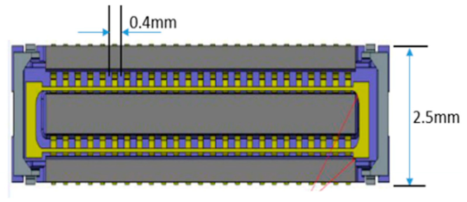
Applsci 12 01216 g003
Figure 4. The pitch and the width of the 0.4 mm BtB connector.
Applsci 12 01216 g004
Figure 5. Front and side view for movement limitation.
Applsci 12 01216 g005
Figure 6. The position of the BtB on the device.
Applsci 12 01216 g006
Figure 7. The backside pin of the BtB.
Applsci 12 01216 g007
Figure 8. Physical and communication system of the proposed approach.
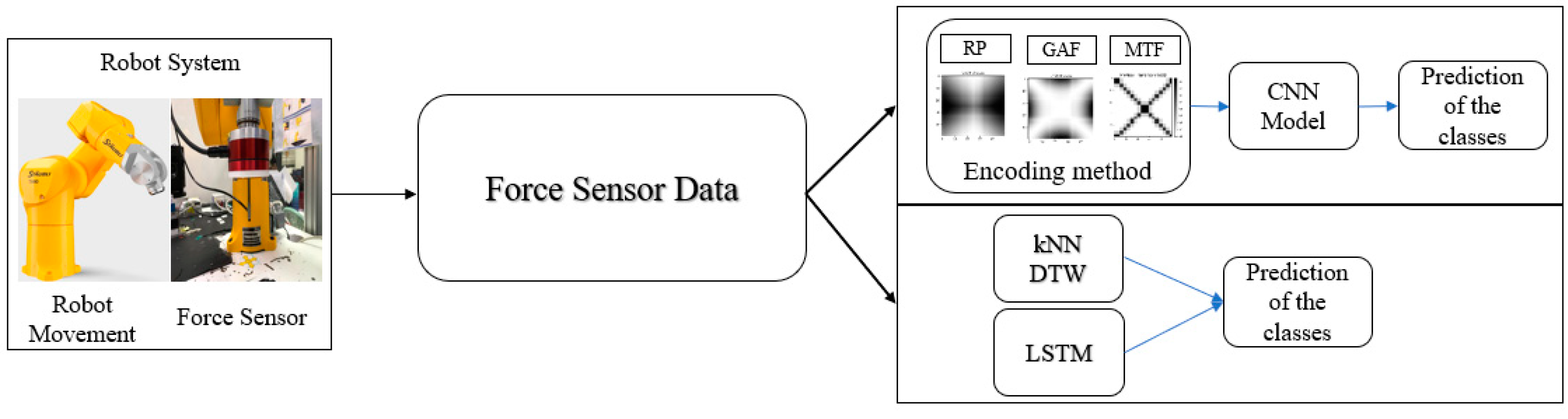
Applsci 12 01216 g008
Figure 9. System diagram.
Applsci 12 01216 g009
Figure 10. Mating process.
Applsci 12 01216 g010
Figure 11. Dataset collection area.
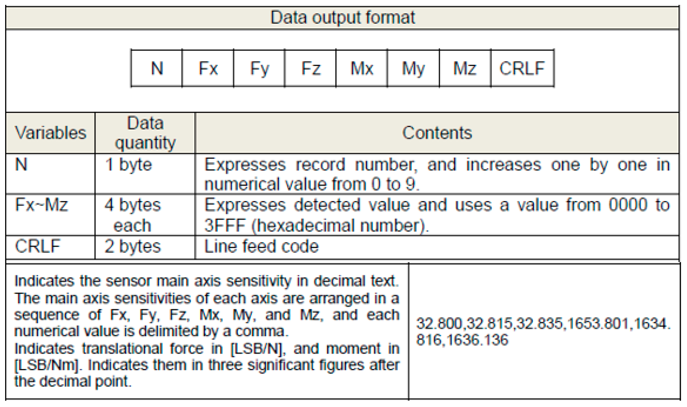
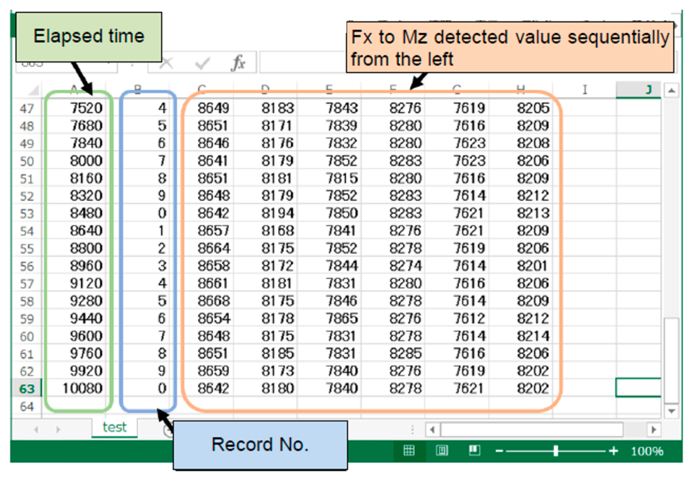
Applsci 12 01216 g011
Figure 12. Force sensor data.
Applsci 12 01216 g012
Figure 14. Force class.
Applsci 12 01216 g014
Figure 15. Illustration sample of the force data as time-series data.
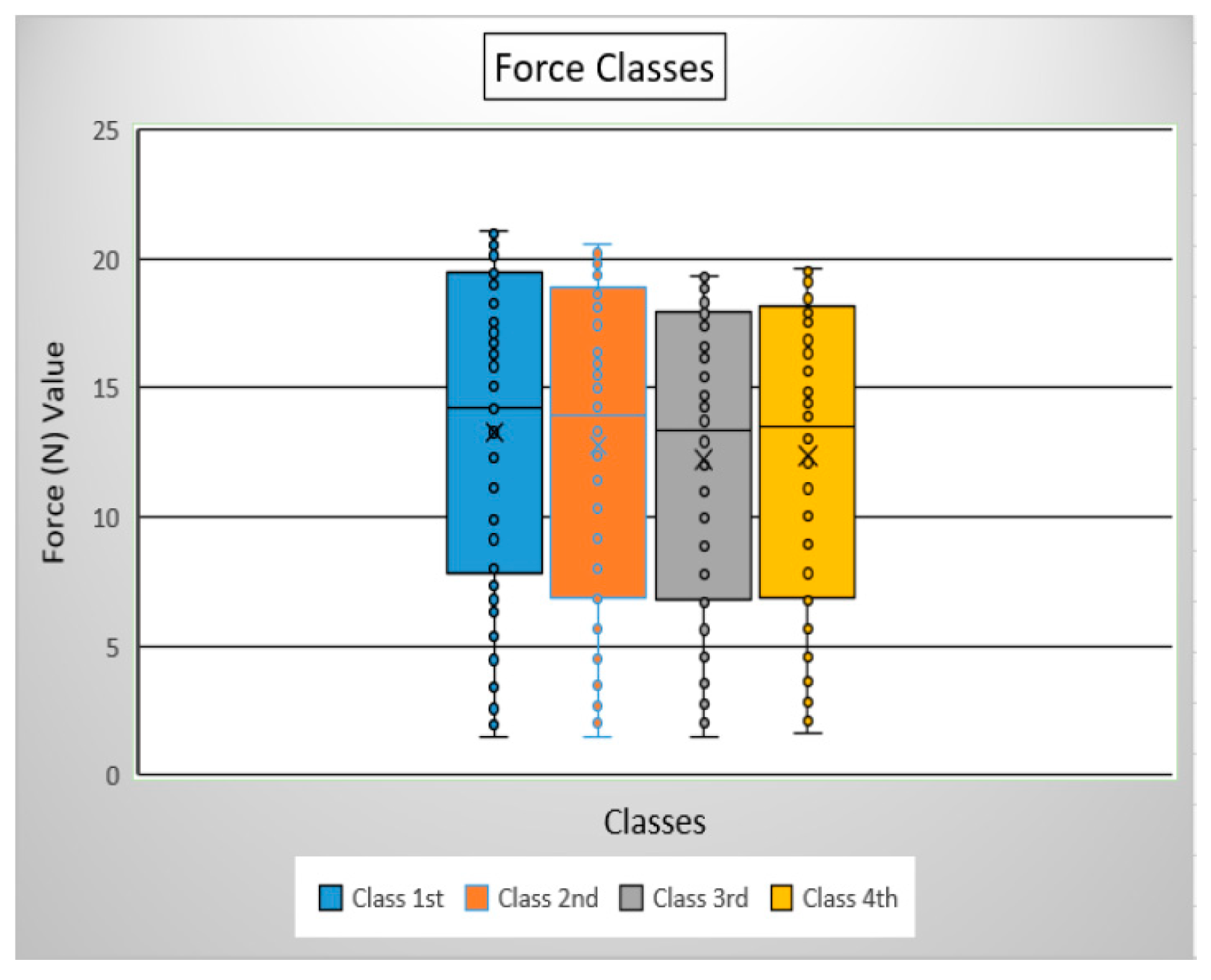
Applsci 12 01216 g015
Figure 16. The class distribution of the training and test data.
Applsci 12 01216 g016
Figure 17. Encoding method in each class.
Applsci 12 01216 g017
Figure 20. Encoding methods in each class utilizing Gramian angular difference field (GADF).
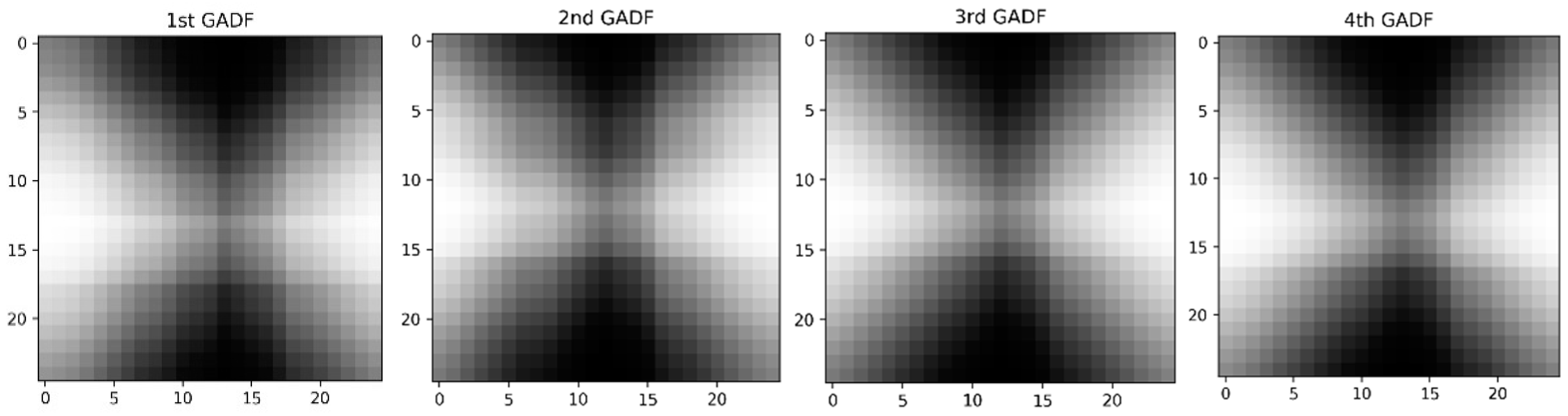
Applsci 12 01216 g020
Figure 21. Encoding methods in each class utilizing GADF.
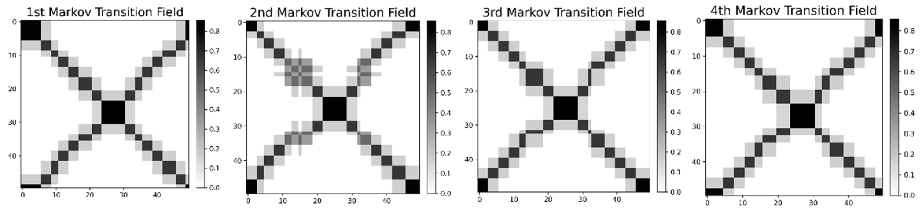
Applsci 12 01216 g021
Figure 22. Encoding methods in each class utilizing Markov transition field (MTF).
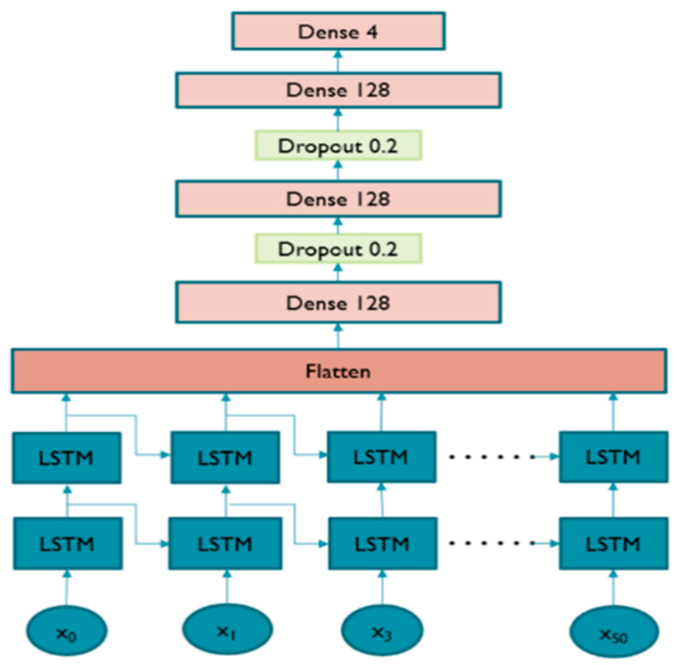
Applsci 12 01216 g022
Figure 23. The architecture of the long short-term memory (LSTM).
Applsci 12 01216 g023
Figure 24. Model accuracy (left), loss (middle), and confusion matrix (right) of SoftMax tuned recurrence plot (RP) model.
Applsci 12 01216 g024
Figure 25. Model accuracy (left), loss (middle), and confusion matrix of the SGD-tuned RP model with L2-SVM (right).
Applsci 12 01216 g025
Figure 26. Model accuracy (left), loss (middle), and confusion matrix of the RP model with L2-SVM (right).
Applsci 12 01216 g026
Figure 27. Model accuracy (left), loss (middle), and confusion matrix (right) of the GASF CNN model.
Applsci 12 01216 g027
Figure 28. Accuracy (left), loss (middle) and confusion matrix (right) of the GADF CNN model.
Applsci 12 01216 g028
Figure 29. Accuracy (left), error (middle) and confusion matrix (right) of the MTF CNN model.
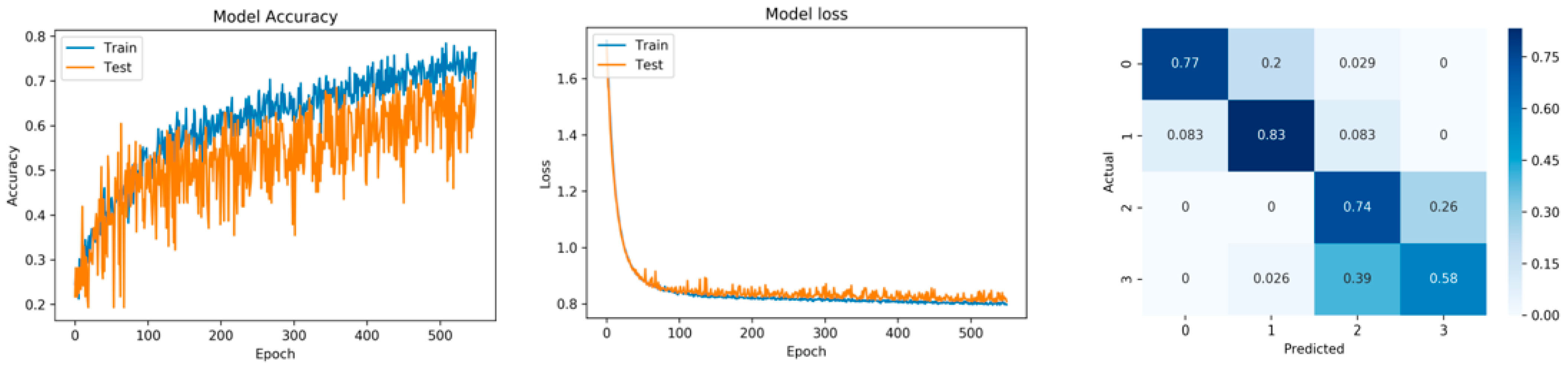
Applsci 12 01216 g029
Figure 30. Accuracy, error and confusion matrix of the LSTM model.
Applsci 12 01216 g030
Figure 31. The successful mating process with its insertion max force.
Applsci 12 01216 g031
Table 1. Highlights of the literature review.
Mating Category
ReferenceCategorySub CategoryNovelty on Insertion Process
[2]TechniquePosition Error MitigationPassive Compliance Control
[3]TechniquePosition Error MitigationVariable Remote Control
[4]TechniquePosition Error MitigationRemote Center Compliance
[5]TechniquePosition Error MitigationError Recovery Strategy
[6]TechniqueBlind Search StrategiesThe Tilt Strategy
[7]TechniqueBlind Search StrategiesSpiral, Probing, and Binary Search
[8]TechniqueVision-Force GuideHybrid Force and Vision
[9]TechniqueVision-Force GuideHybrid Force and Vision
[10]TechniqueVision-Force GuideRobotic Gripper
[11]TechniqueVision-Force GuideRobotic Gripper
[12]TechniqueVision-Force GuideRobotic Gripper
[13]Data AnalysisProbabilistic ApproachAnalysis on Connector States
[14]Data AnalysisLogistic RegressionAnalysis on Visual, Audio, and Force
[15]Data AnalysisGeneralization Fuzzy Analysis for Diagnosis
[16]Data AnalysisPredictionSpeed Analysis
[17]Data AnalysisMachine LearningReinforcement Learning
[18]Data AnalysisMachine Learning Fuzzy Logic Driven Approach
[19]Data AnalysisMachine Learning Deep Q Learning Prediction
[20]Data AnalysisMachine LearningMeta-Reinforcement Learning
[21]Data AnalysisMachine LearningGenerative Adversarial Learning
[22]Data AnalysisMachine LearningLearning From Human Demonstration
[23]Data AnalysisMachine LearningAssembly Motion Demonstration
[24]Data AnalysisMachine LearningAssembly Motion Demonstration
[25]Data AnalysisMachine LearningCompliance Approach from Human Demonstration
[26]Data Analysis Encoding ApproachGAF and MTF
[27]Data AnalysisEncoding ApproachGAF and MTF
[28]Data AnalysisEncoding ApproachGAF and MTF
[29]Data Analysis Encoding Approach Time Series + Deep CNN
Table 2. Board-to-board connector specification.
Design Specification
Number of Pins50
Number of Pins50
Pitch0.40 mm
Mated height0.80 mm
Total Width2.50 mm
TypeSurface mount (SMT.)
Table 3. Dataset detail.
Data Set
Number of classes, c4
Number of training samples, Ntr400
Number of testing samples, Nts140
Length of training samples, l50
Table 4. Hyperparameters adopted in the GADF convolutional neural network (CNN).
Data Set
Loss functionCategorical cross-entropy
OptimizerAdam (0.001)
Kernel RegularizerL2 (0.01)
Batch size20
Epoch250 (early stopping)
Table 5. Hyperparameters adopted in the MTF CNN network.
Data Set
Loss functionCategorical cross-entropy
OptimizerAdam (0.001)
Kernel RegularizerL2 (0.01)
Batch size20
Epoch350
Table 6. Hyperparameters of the k-nearest neighbor dynamic time warping (kNN-DTW) network.
Hyperparameters Used
Warping Distancek Value
105
7
9
1511
13
15
Table 7. Hyperparameters adopted in the RP CNN L2-SVM.
Hyperparameters Used
Parameters1st Tuned2nd Tuned
LossSquared-hingeSquared-hinge
OptimizerAdamSGD
Kernel RegularizerL2 (0.01)L2 (0.01)
Batch size3220
Epoch420 (early stopping)600
Table 8. Accuracy value RP CNN network.
Accuracy Value of Classes
ClassesSoftMaxL2-SVM (SGD)L2-SVM (Adam)
10.910.770.83
20.700.830.75
30.560.740.74
40.80.580.71
Table 9. Class accuracy value of GAF CNN network.
Accuracy Value of Classes
ClassesGASFGADF
10.830.77
20.580.67
30.740.78
40.610.63
Table 10. Class accuracy value of long short-term memory (LSTM) network.
Accuracy Value of Classes
ClassesLSTM
10.60
20.71
30.52
40.50
Table 11. Class accuracy value of warping distance 10.
Accuracy Value of Classes
Classesk = 5k = 7k = 9
10.490.540.54
20.710.620.58
30.590.560.56
40.470.340.34
Table 12. Class accuracy value of warping distance 15.
Accuracy Value of Classes
Classesk = 11k = 13k = 15
10.570.490.54
20.710.670.67
30.590.670.70
40.470.500.47
Table 13. Class accuracy value of all k values.
Accuracy Value of k
k ValueAvg. Accuracy (%)
551
752
951
1159
1358.25
1560
Table 14. Comparison of all deep learning models.
ModelAccuracyLossAverage Class Acc. (%)Std.
Train TestTrainTest
RP (SoftMax)86800.430.774.2514.88
RP (L2-SVM SGD)78720.900.837310.65
RP (L2-SVM Adam)82760.740.79765.12
GASF74730.530.616911.63
GADF77.673.20.640.72727.41
LSTM60580.640.7058.259.53
MTF49421.181.233813.75
Bold represents best accuracy and lowesr stand dev; The RP (Softmax) model has the best accuracy in training and testing; the RP(L2-SVM Adam) has the lowest standard deviation.
Publisher’s Note: MDPI stays neutral with regard to jurisdictional claims in published maps and institutional affiliations.

