A Flexible Localization Method of Multi-Constrained Free-Form Surface Based on the Profile Curves

Abstract

The precision forming process is currently used for many difficult-to-cut parts such as aero-engine blades. However, satisfying the tolerance requirement of the forming accuracy is difficult. Thus, precision machining is used to ensure final accuracy of the part. The error of the near-net shape caused by the thermal process cannot be ignored in the machining process. If the cutting tool path is generated in terms of the design blade model, it would be too difficult to satisfy the material allowance and tolerance requirement of the design blade. In this paper, we propose a new flexible localization method to reconstruct a to-be-cut surface which improves the qualification rate. In this method, the tolerance and material allowance requirements are transformed into optimization constraints. Furthermore, the profile curves of the to-be-reconstructed blade surface are converted into the optimization variables. The material allowance distribution of the to-be-reconstructed surface needs to be as uniform as possible. Through this optimization, the profile curves of the blade surface at the specified height are obtained and used to evaluate the to-be-cut blade model. Finally, a typical compressor blade model is used to verify the proposed method. The results show that the approach can meet the tolerance requirements and ensure sufficient material allowance for the near-net shape blades.

1. Introduction

Blades are important parts in aerospace production, and determine performance. Regardless of the processing method used to fabricate the blade, it is essential to ensure that the section profiles of the manufactured blade are within the specified profile tolerance. The blade is a typical free-form surface part and the criterion for eligibility is whether its profile curves meet the design tolerance.

To reduce the difficult-to-cut material left on the blade billet, it is always forged to near-net shape before finishing the cutting. The cost is less when there is less material left from cutting. However, the risk of material shortage is higher when striving to reduce the amount of material left. If the blade billet cannot cover the design blade, the cutting would fail if it is machined by a toolpath generated based on the design blade. To save the expensive blade billet, a new to-be-cut blade surface different from the design blade is required for generating the toolpath. This new surface needs to satisfy both the material allowance and the tolerance requirements.

A coordinate measuring machine (CMM) is usually used to judge whether the blade is qualified in terms of the section profile. The tolerance bands are different in both the specified sections and the segments of same section (Figure 1). On the other hand, the uniform to-be-cut material is benefited by keeping a stable cutting force. Thus, the to-be-cut blade surface needs to satisfy two requirements. The first is that the profile curve of the blade on each specified section should satisfy the tolerance requirement. The second is that the billet should completely cover the to-be-cut blade surface.

This paper proposes a flexible localization method that ensures the non-uniform profile tolerance and uniform material allowance on the section profiles of blade. It is used to obtain an adequate to-be-cut surface as far as possible, even if the shape of the to-be-cut surface is different from the design surface. The near-shape blade billet is clamped on the machine tool and is measured by the on-machine measurement. The measured result representing the blade billet shape is introduced into localization optimization. After the optimization, a to-be-cut blade surface is obtained that is the used to generate the subsequent toolpath.

2. Literature Review

Many researchers have devoted much effort to workpiece localization in the past. Workpiece localization matches the billet and the to-be-cut model before the machining. It is categorized as a nonlinear least-squares problem to keep to-be-cut material uniform. Using a localization optimization algorithm, the appropriate orientation and position of the workpiece can be obtained which satisfy a user-defined set of constrains. In the past, the most popular method was the iterative closest point (ICP) method, which was first proposed by Paul and McKay [1]. Kang et al. [2] analyzed the sensitivity of this method and concluded that the ICP algorithm is efficient and robust. Subsequently, Chu et al. [3] put forward the iterative closest line (ICL) and iterative closest triangle (ICT) algorithms because the ICP algorithm is sensitive to the direction of the initial black model. However, the iteration speed of the algorithm depends on the number of measurement points. Thus, the ICP algorithm is robust, but its efficiency is not very high.

To solve this problem, scholars have made further improvements to the algorithm. Sun et al. [4] proposed three algorithms, including the variational algorithm, the tangent algorithm, and the Hong Tan algorithm. A comparison of the reliability and validity of these algorithms shows that the Hong Tan algorithm has higher accuracy and efficiency. Consequently, Mor and Mosheiov [5] proposed the particle swarm optimization (PSO) algorithm to achieve the accurate localization of the workpiece. Compared with the ICP algorithm, the PSO algorithm has a higher computational efficiency. However, the above algorithms easily become divergent if they do not have an appropriate initial value. In order to overcome this issue, Han et al. [6] developed a novel method whose objective function is the minimum distance. This method does not require an initial value and has a high precision and convergence rate in the calculation process. However, the drawback of the method is that it depends on a correction coefficient. The iterative process becomes divergent if the correction coefficient is chosen incorrectly. Subsequently, Xu et al. [7] proposed a new localization method that is divided into two steps. In this method, the rough alignment is finished according to the Gauss curvature and the mean curvature of the model. The drawbacks of this method lie in the error from the curvature calculation of the nominal model and of the machined model. Besides, the curvature threshold of two corresponding points is always artificially determined. Thus, it fails easy in the rough alignment. Similarly, Chu et al. [8] also proposed two stages in the localization process. The rough localization is finished according to the three corners of the model. It is then combined with a genetic algorithm and simplex method to complete the precise alignment. However, the above algorithm degrades for models with symmetric structure. Subsequently, a unified algorithm for all kinds of symmetrical parts was proposed by Li et al. [9], which can be expressed by the same optimization objective function if the symmetrical subgroups of the work pieces are known. These studies improve the efficiency of localization.

The above research is aimed at the alignment of the unconstrained model. However, due to the existence of multi-source error, it is likely that the design model cannot be wrapped in the billet model during an unconstrained alignment process. To deal with this problem, Li et al. [10] introduced the machining allowance problem which is defined as hybrid localization. The process is split into a location problem and a tolerance problem by using differential geometry and Lie group. Subsequently, Li and Griffiths [11] formulated the general 3D localization problem using three different optimization algorithms to solve this problem. Nevertheless, the presented method is just for simple geometric models that do not involve a free-form surface. Accordingly, Astanin et al. [12] proposed a workpiece localization optimization algorithm for a free-form surface and a mathematical model was established to ensure that the workpiece had sufficient machining allowance. Combined with the simplex method, it was concluded that the objective function of the logarithmic form had a higher efficiency. Furthermore, Sun et al. [13] proposed sequential quadratic programming (SQP) with a mathematical model of unified weight and made a quality evaluation of the registration. This algorithm is more efficient than the direct search algorithm, but it has low computational efficiency because of the Jacoby matrix and the Hessian matrix calculations in each iteration. Zhang et al. [14] modified the simplex method that is used to evaluate the shape error of the machined model. In summary, previous literature focuses on the simple to-be-cut feature but rarely on the free-form surface feature.

The above works focus on the optimization method, and the constraints are only used to ensure sufficient material allowance. Nevertheless, there are few works considering the profile tolerance in the free-form surface localization. Therefore, it is desirable to find a localization method to obtain an optimal to-be-cut blade surface. This surface is used to generate the toolpath that satisfies the material allowance and tolerance requirements. Contrary to previous studies, in this paper, a more flexible localization method is investigated to find available to-be-cut surfaces.

3. The Localization Problem of the Near-Net Shape Blade Surface

3.1. Establishment of the Localization Optimization Model

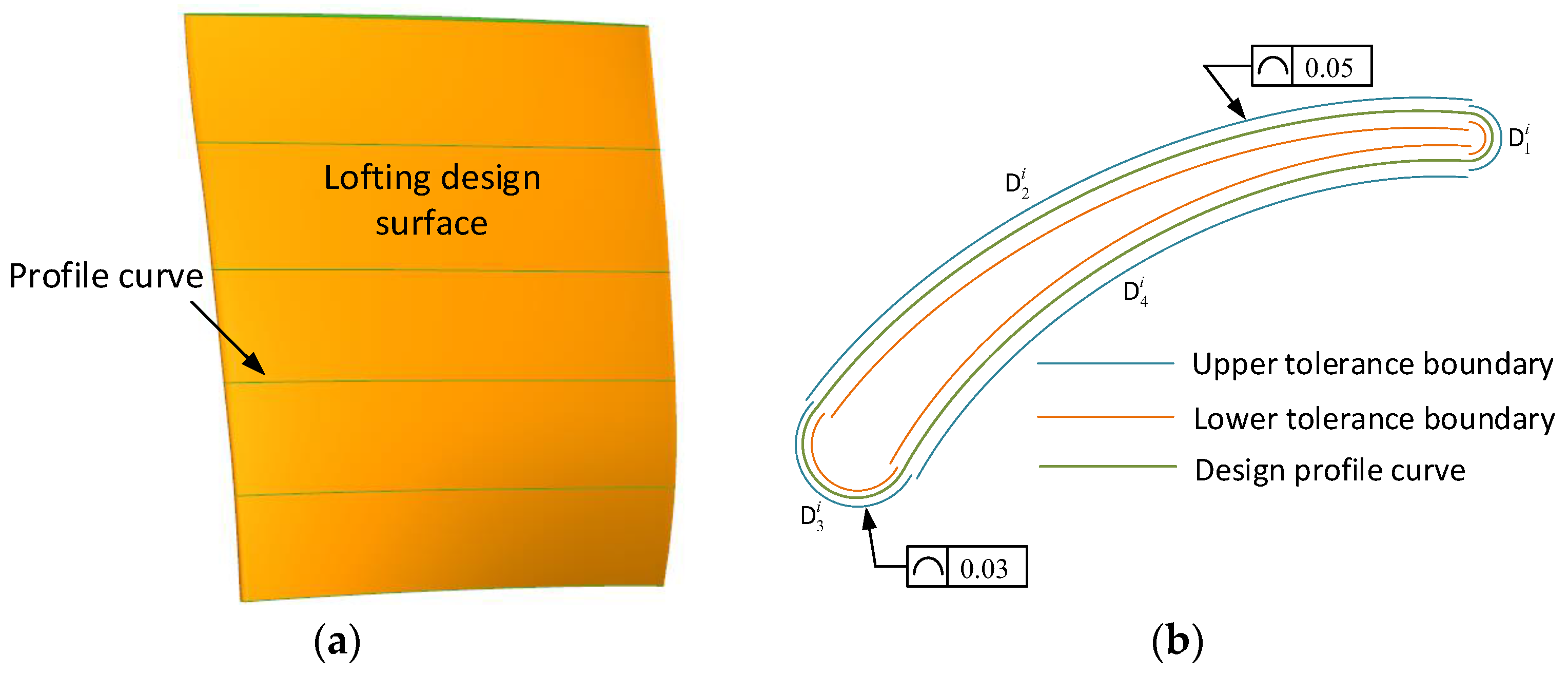
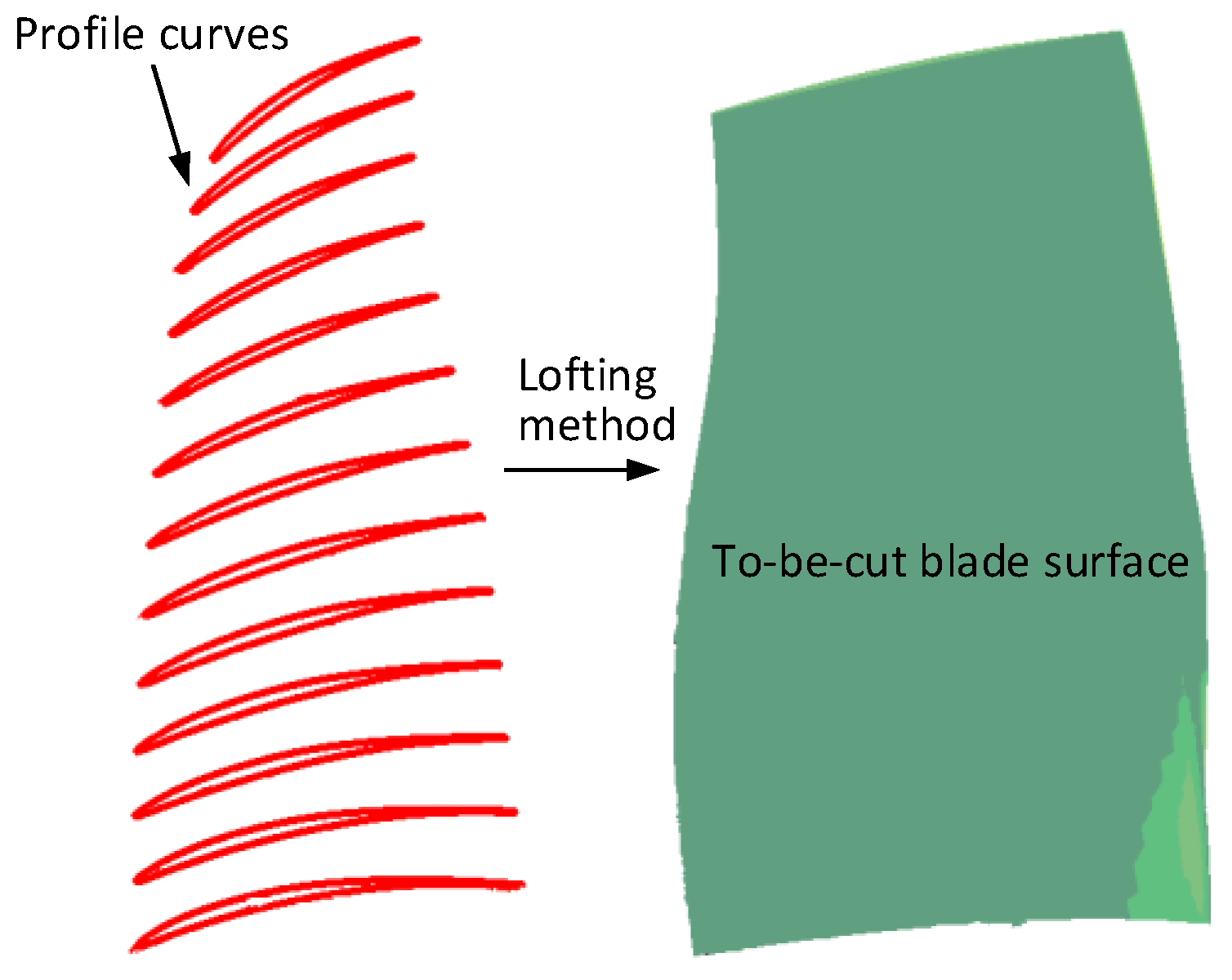
For the free-form surface of a blade, the profile curves on the design blade sections are the basis of controlling the surface shape (Figure 1a). The blade surface is constructed by lofting these profile curves. That is to say, the to-be-cut blade surface can be reconstructed in the same way. Thus, it is important to find a group of appropriate profile curves. The to-be-cut blade surface is represented by $r\left(u,v\right)$.

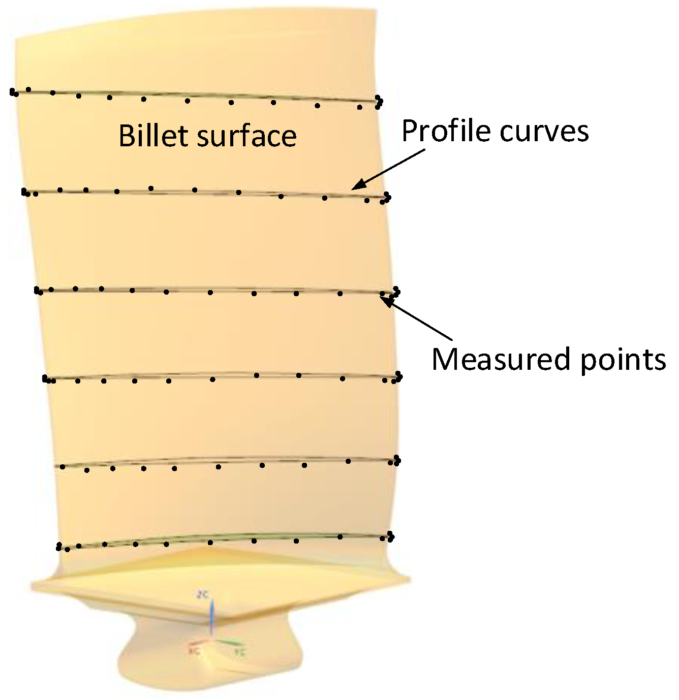
The blade billet shape is used to judge the material allowance for the to-be-cut blade surface. The blade billet shape is always recognized by on-machine measurement. The to-be-measured points are planned on the designed blade profiles. The measured result represents the real material boundary on the profile curves section (Figure 2). They are represented by $P_M=\left\{p_i|i=1,2,\cdots n\right\}$.

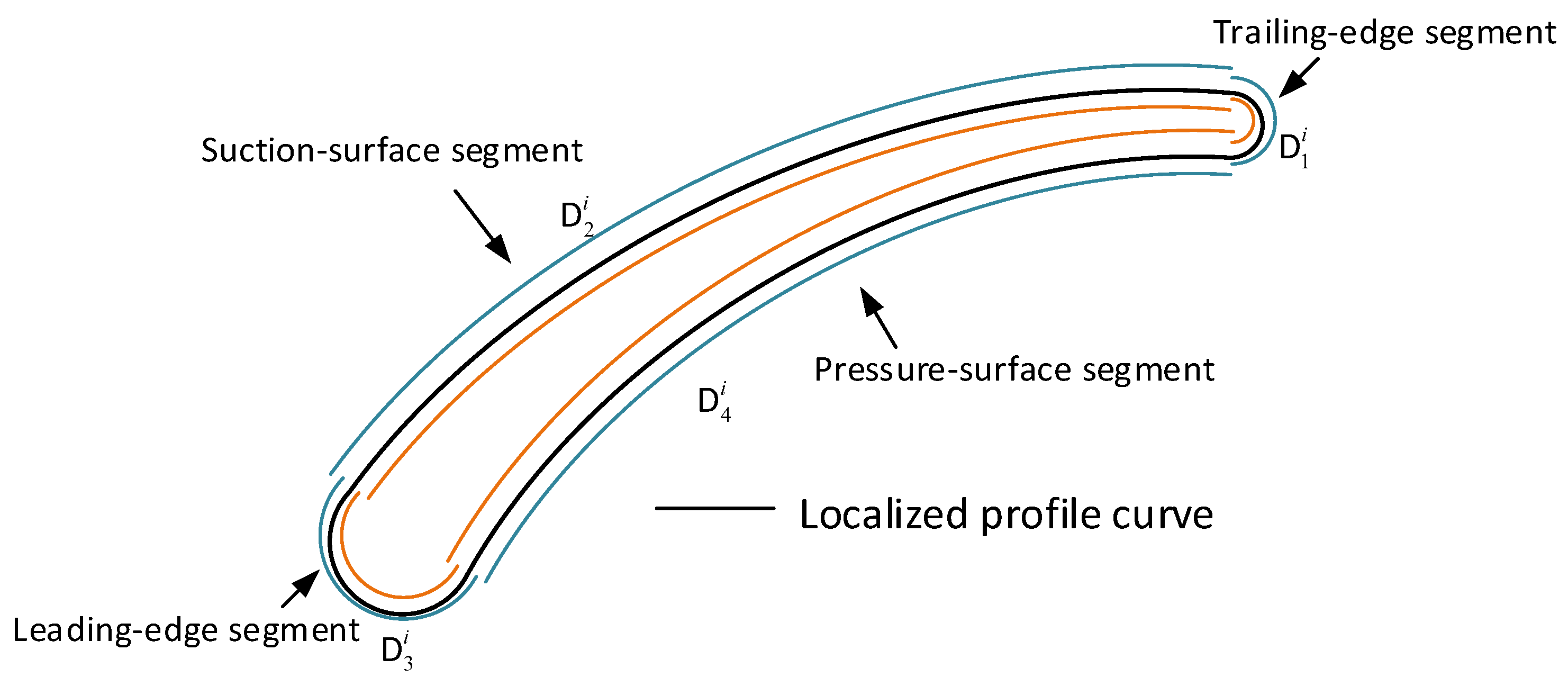
The blade surface is usually divided into the suction-surface segment, the pressure-surface segment, the leading-edge segment, and the trailing-edge segment. Different tolerances are required for these surface areas. After the blade surface localization, the profile of the to-be-cut blade surface segment needs to be within the respective profile tolerance zone (Figure 3).

The to-be-cut material on the blade billet is more uniform, and the cutting status is more stable. Therefore, the objective of the proposed localization is to make the material allowance more uniform. To obtain a favorable to-be-cut blade surface, we establish a flexible localization implemented by a multi-constraint optimization.

Optimization variable: the translation and the rotation matrices of the profile curves on the designed blade sections. The translation matrix is denoted as $T$, and the rotation matrix is denoted as $R$. Each profile curve is localized by its translation matrix and realized by the rotation matrix. The to-be-cut blade surface is reconstructed by the lofting method in terms of the respective profile curves that were localized.

Optimization Objective: The objective of the uniform to-be-cut material is substituted by the distance between the measured points of the blade billet and the to-be-cut blade surface. It is represented by

$$\min f\left(R_j,T_j\right)=\min \left({\displaystyle \sum _{i=0}^n}{\Vert d_i\Vert }^2\right)=\min \left({\displaystyle \sum _{i=0}^n\Vert r\left(u,v\right)-p_i\Vert }\right)$$

(1)

where $d_i$ are the distances from the measured points to the closest points on the to-be-cut blade surface.

Material allowance constraint: The first term is the material allowance constraint. The to-be-cut blade surface should be completely covered by the blade billet. It is represented by

$$h1\left(R_j,T_j\right)=\left(p_i-r\left(u,v\right)\right)\cdot n_i\ge 0$$

(2)

where $n_i$ is the normal of the closest point on the to-be-cut blade surface corresponding to the measured point.

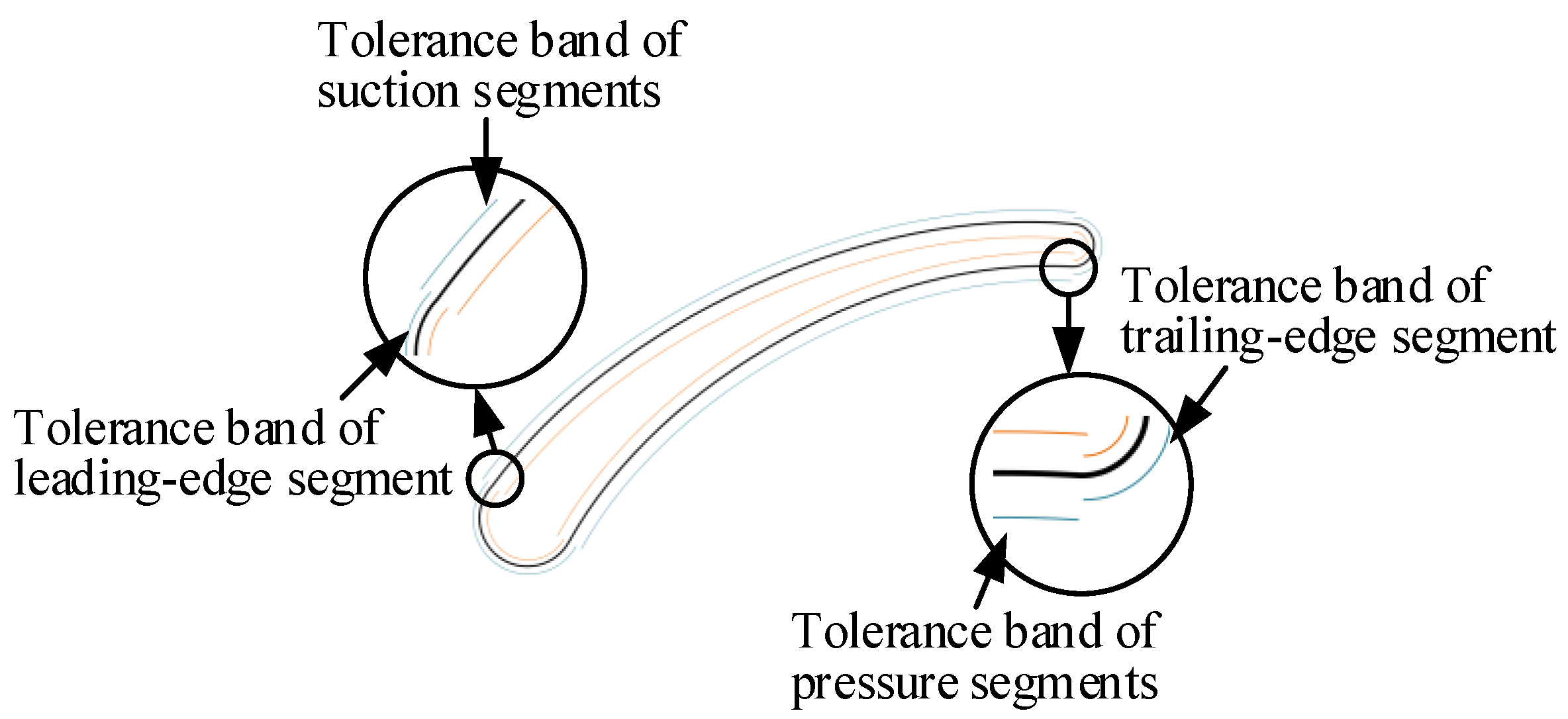
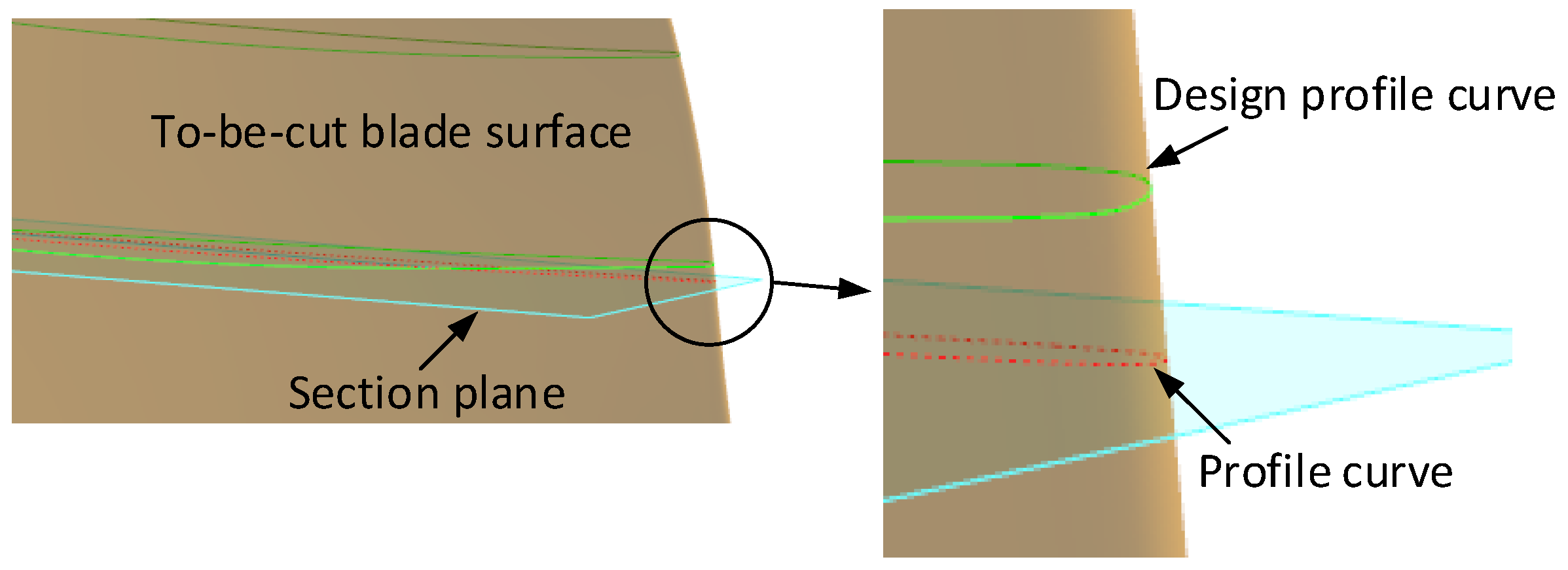
Profile tolerance constraint: The different segments of the profile curves that belong to the optimized blade surface need to be within corresponding profile tolerances (Figure 4). They are represented by

$$h2\left(R_j,T_j\right)=\left(C_{p,k}-S_{p,k}\right)\cdot n_{p,k}\ge 0\begin{array}{cc}& p=1\cdots m,k=1\cdots l\end{array}$$

(3)

$$h3\left(R_j,T_j\right)=\left(C_{q,k}-S_{q,k}\right)\cdot n_{q,k}\le 0\begin{array}{cc}& q=1\cdots m,k=1\cdots l\end{array}$$

(4)

where $S_{p,k}$ represent the closest points on the suction segment and the pressure segment of the profile curves, $S_{q,k}$ represent the closest points on the leading-edge segment and the trailing-edge segment of the profile curves. $C_{p,k}$ and $C_{q,k}$ are the scatter points on the tolerance boundaries. $n_{p,k}$ and $n_{q,k}$ are the unit normal of the scatter point. $k$ is the index of the profile curves and $p,q$ are the index of the scatter points on the profile curve.

There is no accurate expression of the tolerance boundaries. The tolerance boundaries of the profile curves are defined by deviating from the nominal profile curves along the normal vector. The expressions of profile tolerance boundaries are represented by

$$C_{i,k}(t)={\displaystyle \sum _{i=0}^n{N}_{i,3}}(t)V_i+\frac{T}{2}n(t)$$

(5)

$$C_{i,k}(t)={\displaystyle \sum _{i=0}^n{N}_{i,3}}(t)V_i-\frac{T}{2}n(t)$$

(6)

where $n\left(t\right)$ is the unit normal of a given point on the designed profile curve.

The profile curves $S\left(t\right)$ of the blade surface are represented by cubic B-spline curves. They are represented by $S(t)=\{s^0(t),s^1(t)\cdots s^l(t)\}$. The to-be-cut blade surface is represented by $r\left(u,v\right)=f\left[S\left(t\right),i\right]$ where $f$ is the lofting operator in terms of profile curves and $i$ is the index of the profile curves. According to the affine invariance property of B-spline curves, the transformation of the control points has same effect as the transformation of the profile curves. The formula of each transformed profile curve is

$$s_j\left(t\right)={\displaystyle \sum _{i=0}^n}R\left(\alpha \right)\cdot R\left(\beta \right)\cdot R\left(\gamma \right)\cdot T\left(\Delta x,\Delta y,\Delta z\right)\cdot N_{i,3}\cdot V_{i,j}$$

(7)

where $R\left(\alpha \right)=\left[\begin{array}{cccc}\cos \alpha & -\sin \alpha & 0& 0\\ \sin \alpha & \cos \alpha & 0& 0\\ 0& 0& 1& 0\\ 0& 0& 0& 1\end{array}\right]$ and $T\left(\Delta x,\Delta y\right)=\left[\begin{array}{cccc}1& 0& 0& \Delta x\\ 0& 1& 0& \Delta y\\ 0& 0& 1& 0\\ 0& 0& 0& 1\end{array}\right]$.

$R\left(\alpha \right)$, $R\left(\beta \right)$, and $R\left(\gamma \right)$ are the rotation matrices and $T\left(\Delta x,\Delta y,\Delta z\right)$ is the translation matrix. $\alpha$ is the rotation angle around the $\mathrm{X}$ axis, $\beta$ is the rotation angle around the $\mathrm{Y}$ axis, and $\gamma$ is the rotation angle around the $\mathrm{Z}$ axis. $\Delta x$, $\Delta y$, and $\Delta z$ are the translation values of the profile curve along the $\mathrm{X}$, $\mathrm{Y}$, $\mathrm{Z}$ directions, respectively.

3.2. Reconstruction of the To-Be-Cut Blade Surface

In the proposed localization optimization, the initial value is the profile curves on the sections of the design blade. By the Newton iteration method, the transformation parameters are determined as the optimization result. By the lofting method, the to-be-cut blade surface is constructed in terms of the profile curves in the sections (Figure 5). The process of lofting is as follows.

Step 1: The profile curves are generated in the sections represented by expressions $C_i\left(v\right)$.

Step 2: The number of control points of each profile curve are uniformed.

Step 3: The node vector in $v$ directions are uniformed.

Step 4: The number of $u$ directions on the surface, parameters, and node vector are determined.

Step 5: The control points of the surface are optimized in terms of the proposed optimization model.

Step 6: The expression of the surface is obtained in terms of the control points and the original B-spline basis function.

The parameter equation of the to-be-cut blade surface is given by

$$r\left(u,v\right)={\displaystyle \sum _{i=0}^m}{\displaystyle \sum _{j=0}^n}{N}_{i,3}\left(u\right)\cdot N_{j,3}\left(v\right)\cdot V_{i,j}$$

(8)

The above formula can also be written as

$$r\left(u,v\right)={\displaystyle \sum _{i=0}^m}\left({\displaystyle \sum _{j=0}^n}{N}_{j,3}\left(v\right)\cdot V_{i,j}\right)\cdot N_{i,3}\left(u\right)$$

(9)

It can also be written as

$$r\left(u,v\right)={\displaystyle \sum _{i=0}^m}{c}_i\left(v\right)\cdot N_{i,3}\left(u\right)$$

(10)

where $C_i\left(v\right)$ are the profile curves of the to-be-cut blade surface. $V_{i,j}$ are the control points of the profile curves. The translation and rotation operators in the optimization are applied on these control points.

3.3. The Profile Curve Calculation of the To-Be-Cut Surface

In the design coordinate system of the blade, the $\mathrm{XOY}$ plane is chosen to be perpendicular to the blade stack axis. The $\mathrm{X}$ axis is defined as parallel to the average cord or the axis of the engine, and the positive direction is from the leading edge to the trailing edge. If the $\mathrm{X}$ axis is not parallel to the axis of the engine, then the angle between the $\mathrm{X}$ axis and the axis of the engine must be rounded to the degree. The $\mathrm{Z}$ axis is set to be perpendicular to the engine axis and the $\mathrm{Y}$ axis is positively determined based on the right-hand rule. Thus, for the to-be-cut blade surface, a series of section planes would intersect with the blade surface. The intersection profile is the profile curve which is perpendicular to the $\mathrm{Z}$ axis.

The optimization constraints are judged within the blade sections. If the to-be-cut blade surface is covered by the blade billet and inside the profile tolerance band on all blade sections, it would be an available surface. Therefore, the profile curves on the blade sections need to be calculated (Figure 6). The profile curve in this paper is calculated by the Newton iteration method.

The parametric equation of the blade surface is

$$s\left(u,v\right)={\displaystyle \sum _{i=0}^m}{\displaystyle \sum _{j=0}^n}{N}_{i,3}\cdot N_{j,3}\cdot V_{i,j}$$

(11)

where $V_{i,j}=\left(x_{i,j},y_{i,j},z_{i,j}\right)$ are the control points of the surface.

The equation of blade sections is:

$$z=z_m$$

(12)

The intersection of the surface $s(u,v)$ and the plane $z_m$ satisfies

$$s_z=z_m$$

(13)

Which is used to determine the surface parameter value $\left(u,v\right)$.

The transformations of the profile curves on the blade sections are very small. In the optimization, the parameter $u$ of the nominal blade is inherited. The parameter is discretized into a sequence $\left[u_0,u_1,\cdots u_n\right]$ in the range $\left[0,1\right]$. Then the initial value of the Newton iterative method is $\left[\begin{array}{c}{u}_0,u_1\cdots u_n\\ v_i,v_i\cdots v_i\end{array}\right]$. The coordinates of the points $\left(x_i,y_i\right), i=0,1,\cdots n$ on the surface are obtained by substituting $(u,v)$. Finally, the expression of profile curve is obtained according to the calculus of interpolation of the coordinate points on the surface.

3.4. Implementation of Optimal Localization Algorithm

The blade localization before the finish machining is essentially an optimization. The input of this optimization is a set of profile curves $c_i\left(v\right)$ of the nominal surface, the measured points $p_i$ of the blade billet, and the segmented profile tolerance requirements. The output of this optimization is the position of the optimized profile curves.

The profile curves of the to-be-cut blade can be obtained as follows:

Step 1: A B-spline surface $S\left(u,v\right)$ is constructed through a set of profile curves $C_i\left(v\right)$. The initial translation value is $T^{\left(0\right)}$ and the initial rotation value is $R^{\left(0\right)}$.

Step 2: According to the affine deformation of the B-spline curves and surfaces, the new profile curves ${C_i}^{\prime }\left(v\right)$ are obtained by the space transformation of the control points of the curve $C_i\left(v\right)$ and obtaining the new lofting $S^{\prime }\left(u,v\right)$ according to the ${C_i}^{\prime }\left(v\right)$.

Step 3: By the Newton iterative method, the closest points ${p_i}^{\prime }$ on surface $S^{\prime }\left(u,v\right)$ are obtained, and the least squares distance from the measuring points $p_i$ to the closest point ${p_i}^{\prime }$ is calculated.

Step 4: According to the material allowance constraint, the constraint condition $h3$ is obtained. Moreover, the constraint equations $h1$ and $h2$ are obtained according to the profile curves within the profile tolerance band.

Step 5: According to the objective function and the constraint equations $h1$, $h2$, and $h3$, the optimization variables are updated during the optimization.

Step 6: It is judged whether the calculation results satisfy the constraint and satisfy the $\Vert x^{\left(k\right)}-x^{\left(k-1\right)}\Vert \le \epsilon$; if it is satisfied, the iterative process converges to an optimal solution.

Step 7: If the conditions of step 6 are not met, then according to the updated $x^{(k)}$ the process returns directly to step 2. If the number of iterations $k\le N$ is satisfied, then the optimization solution $x^{(k)}$ is obtained. Otherwise, there is no solution to the optimization.

4. Experiment

To find a favorable to-be-cut surface before machining, we considered three optimization methods: unconstrained optimization, material-constraint optimization, and multi-constraint optimization. They are explained in detail as follows.

Unconstrained optimization: The to-be-cut blade surface is localized in terms of minimizing the distance from the blade billet.

Material-constraint optimization: In addition to minimizing the distance between to-be-cut blade surface and the blade billet, the to-be-cut blade surface is localized to ensure there is sufficient material.

Multi-constraint optimization: In comparison with the material-constraint optimization, a profile tolerance constraint is added into the optimization model.

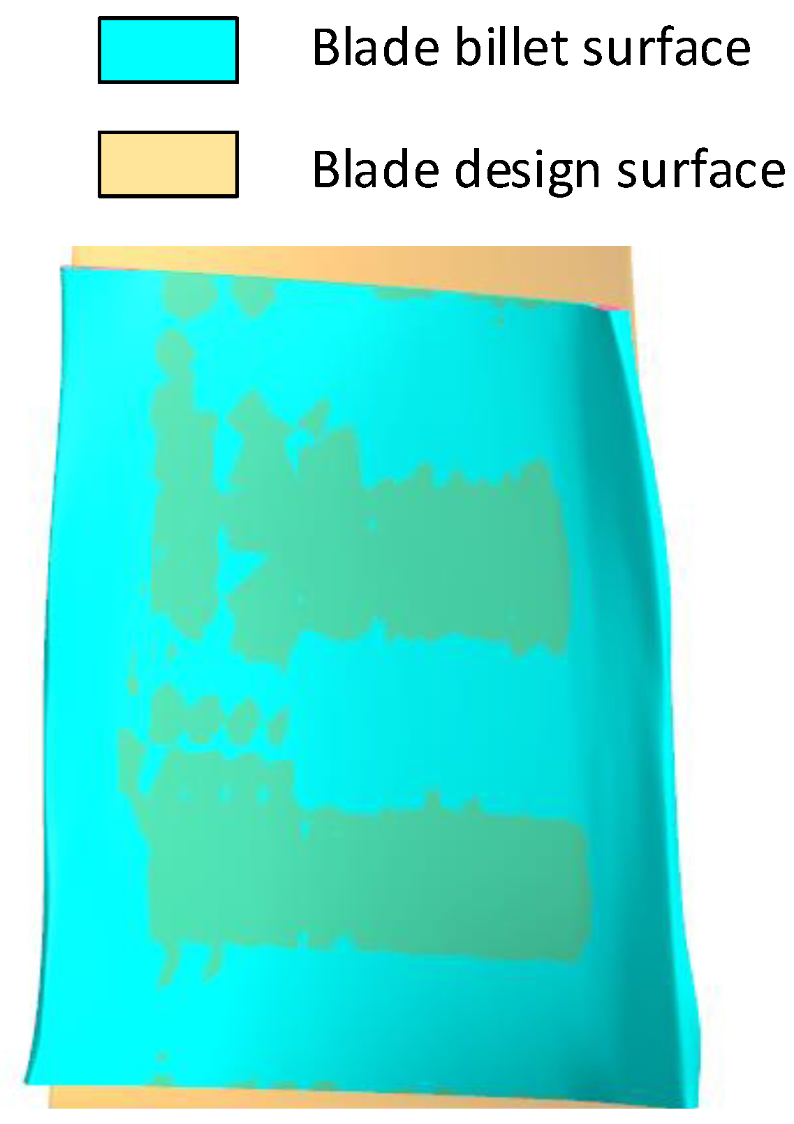
In our experiment, a compressor blade was used to verify the advantage of a proposed localization model that could guarantee sufficient material allowance and blade profile tolerances. The measured points and the blade design surface before the localization are shown in Figure 7.

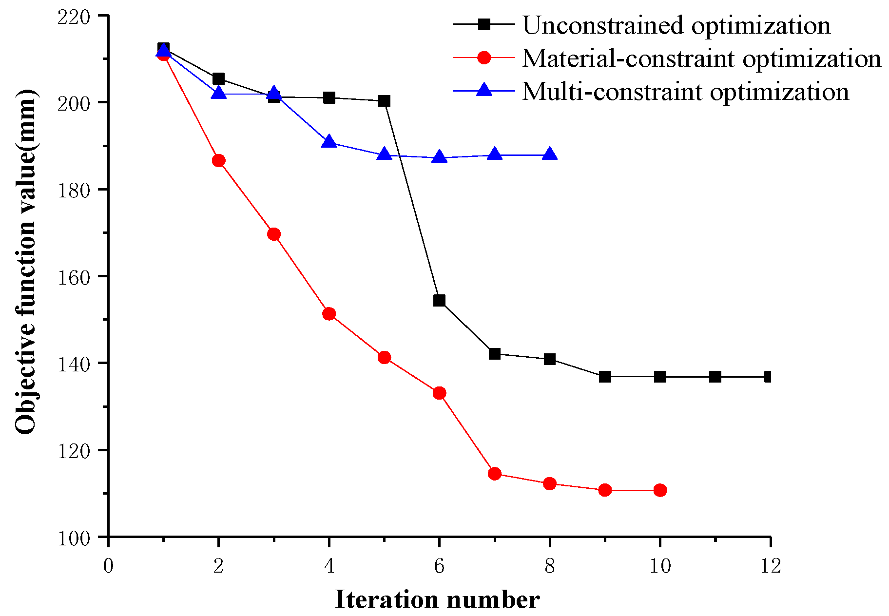
Figure 7 demonstrates that there was an absence of material allowance in some areas of the design blade model. If the design blade model was used directly to generate the toolpath, the machining would fail. Thus, it was necessary to implement the localization before the subsequent machining. The above three optimizations of localization were implemented. The convergence rates of the three optimizations are shown in Figure 8. In the unconstrained optimization, the square sum of the unsigned distances that only let the to-be-cut blade surface be in the center of the blade billet was minimized. In the material-constraint optimization, the square sum of the signed distances with all positive distances was minimized. In the multi-constraint optimization, the objective function was achieved with fewest iterations.

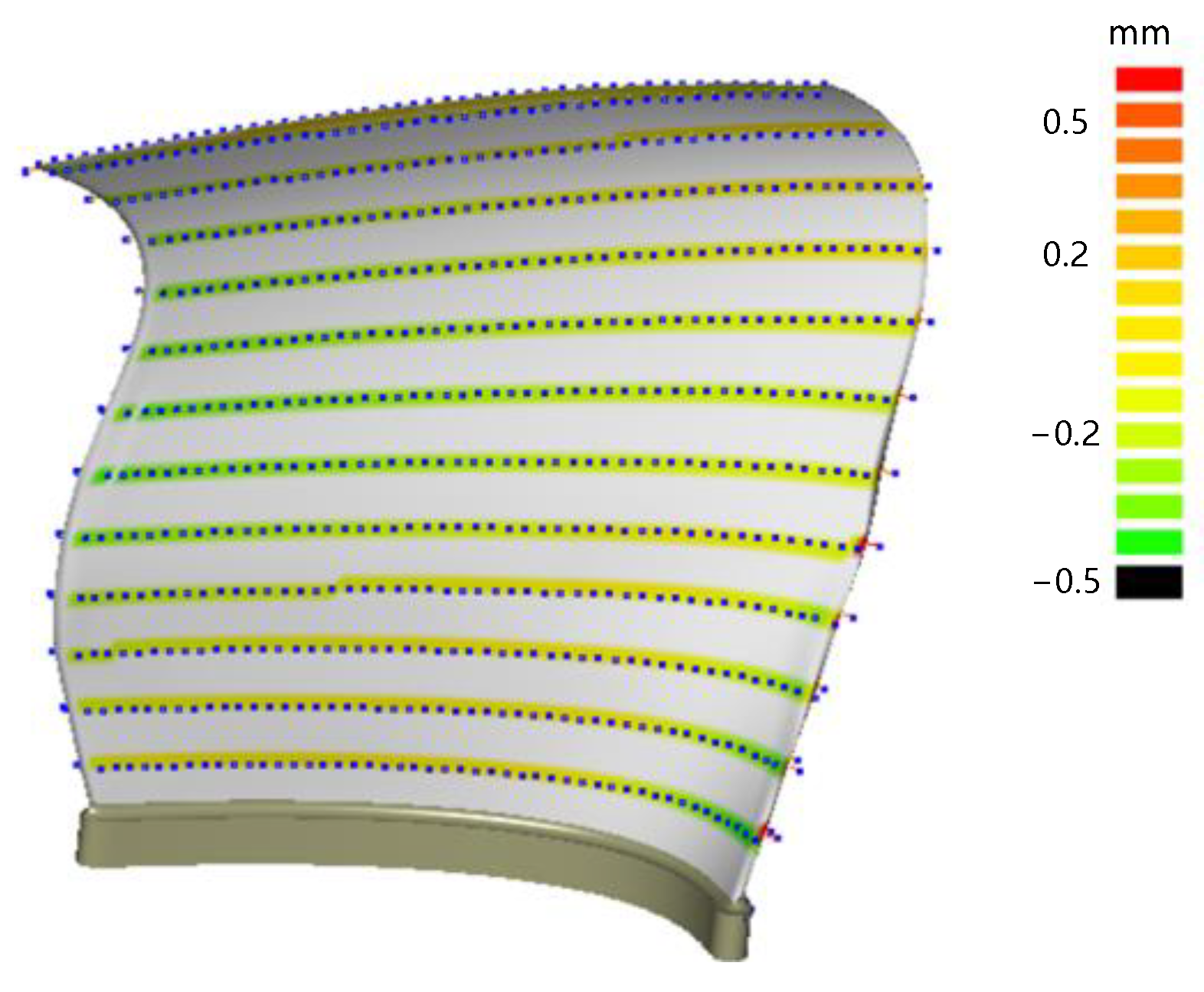
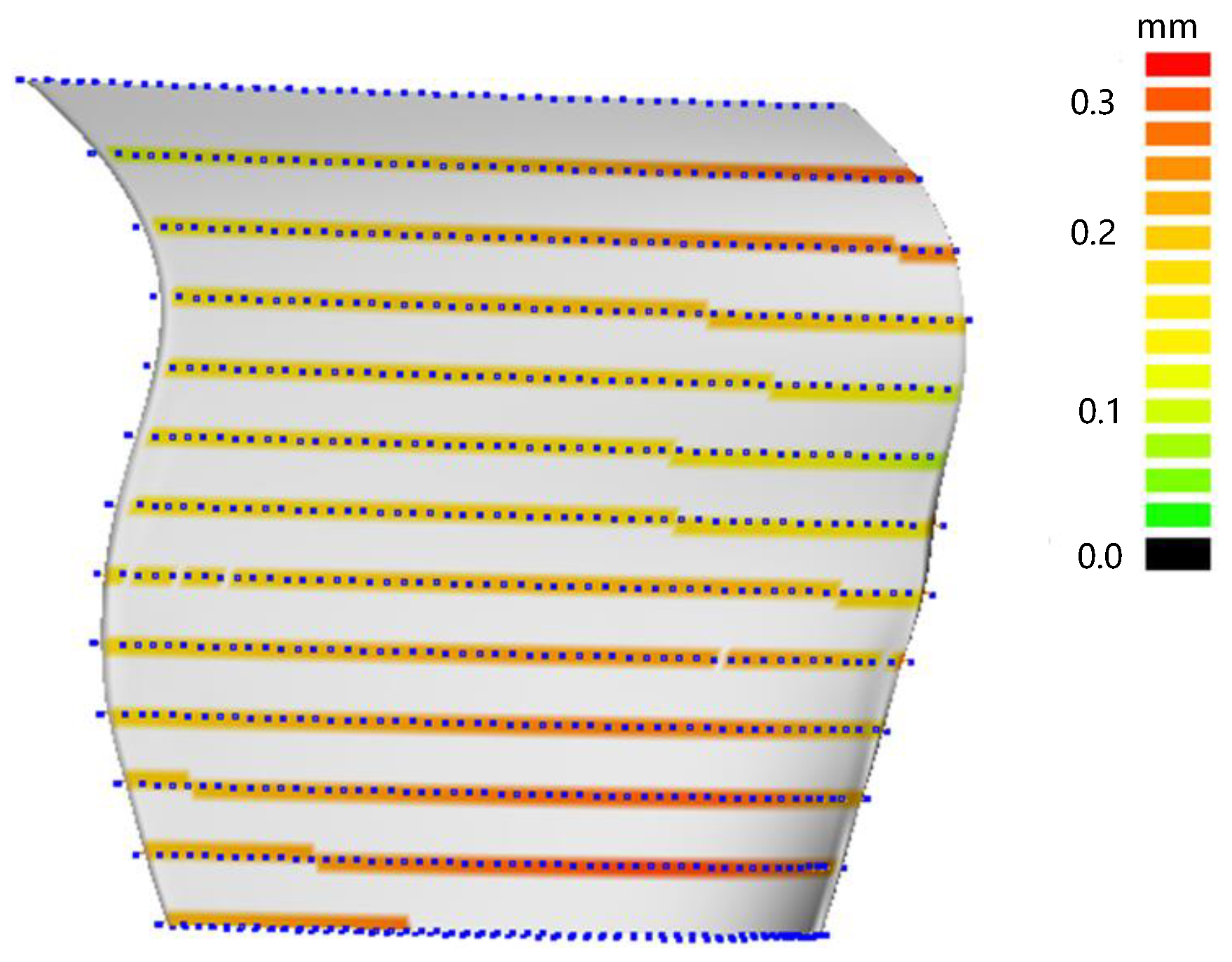
The optimized to-be-cut blade surfaces after optimization are shown in Figure 9. The chart color represents the material allowance left on the optimized to-be-cut blade surface. In the case of the unconstrained optimization, the profile curves were adjusted to put the to-be-cut blade surface in the middle of the blade billet (Figure 9). However, there was not enough material because this was be ensured in the optimization model. 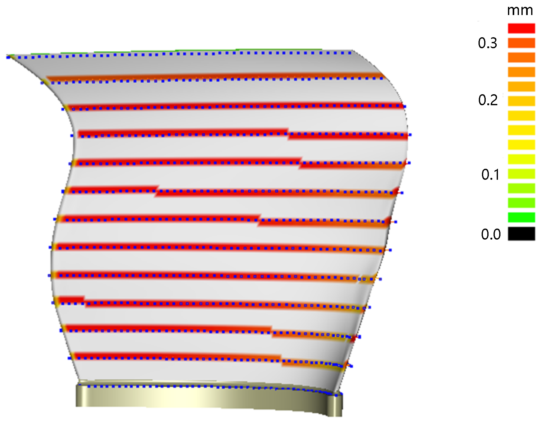In the case of material-constraint optimization, there was sufficient material for subsequent machining (Figure 10). There was enough material because of the material constraint in the optimization model. In the case of the multi-constraint optimization, the material allowance was satisfied for subsequent machining (Figure 11). This achieved the same effect as the previous optimization method.

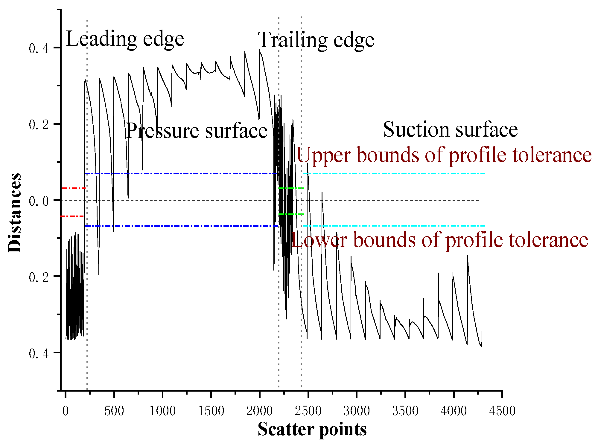
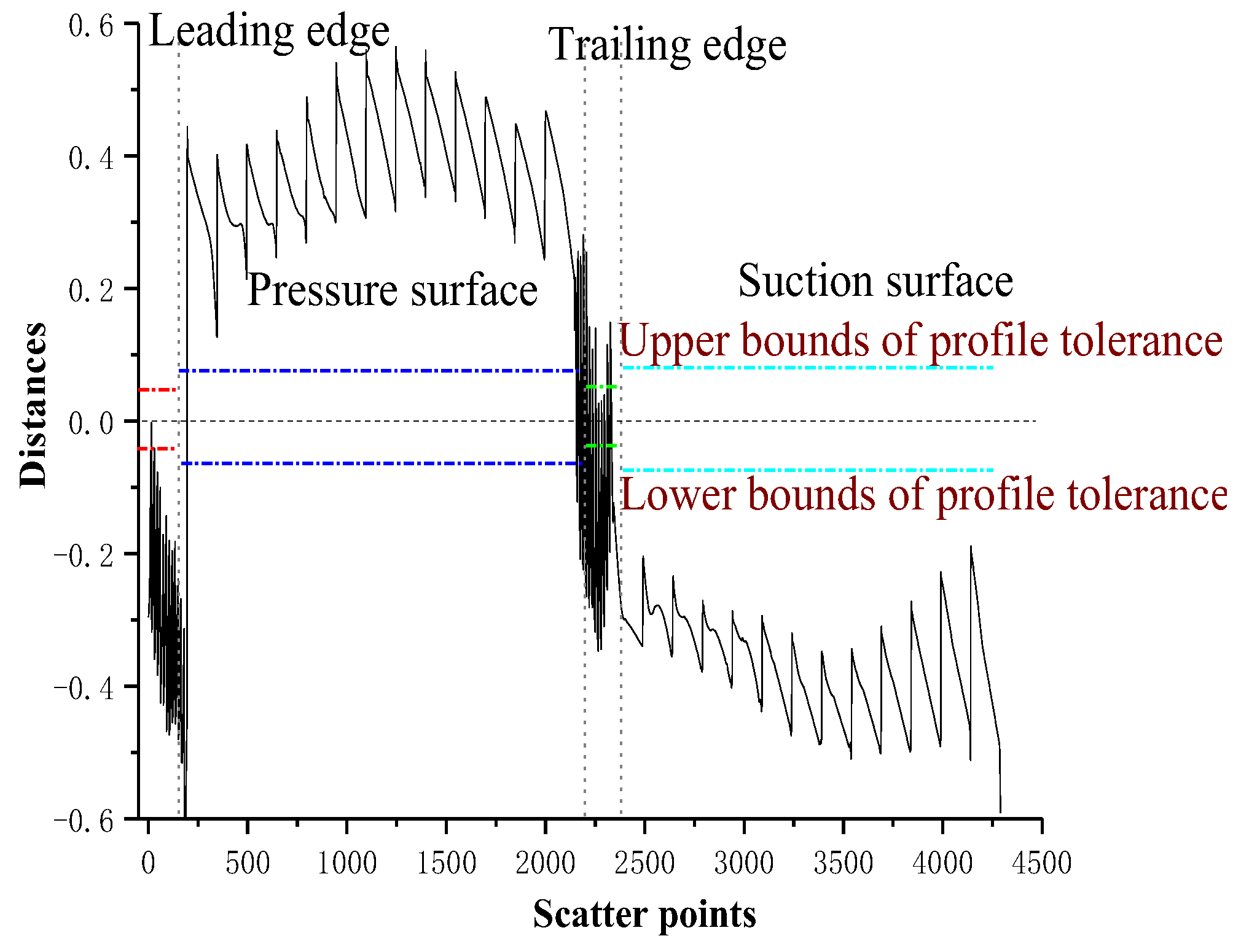
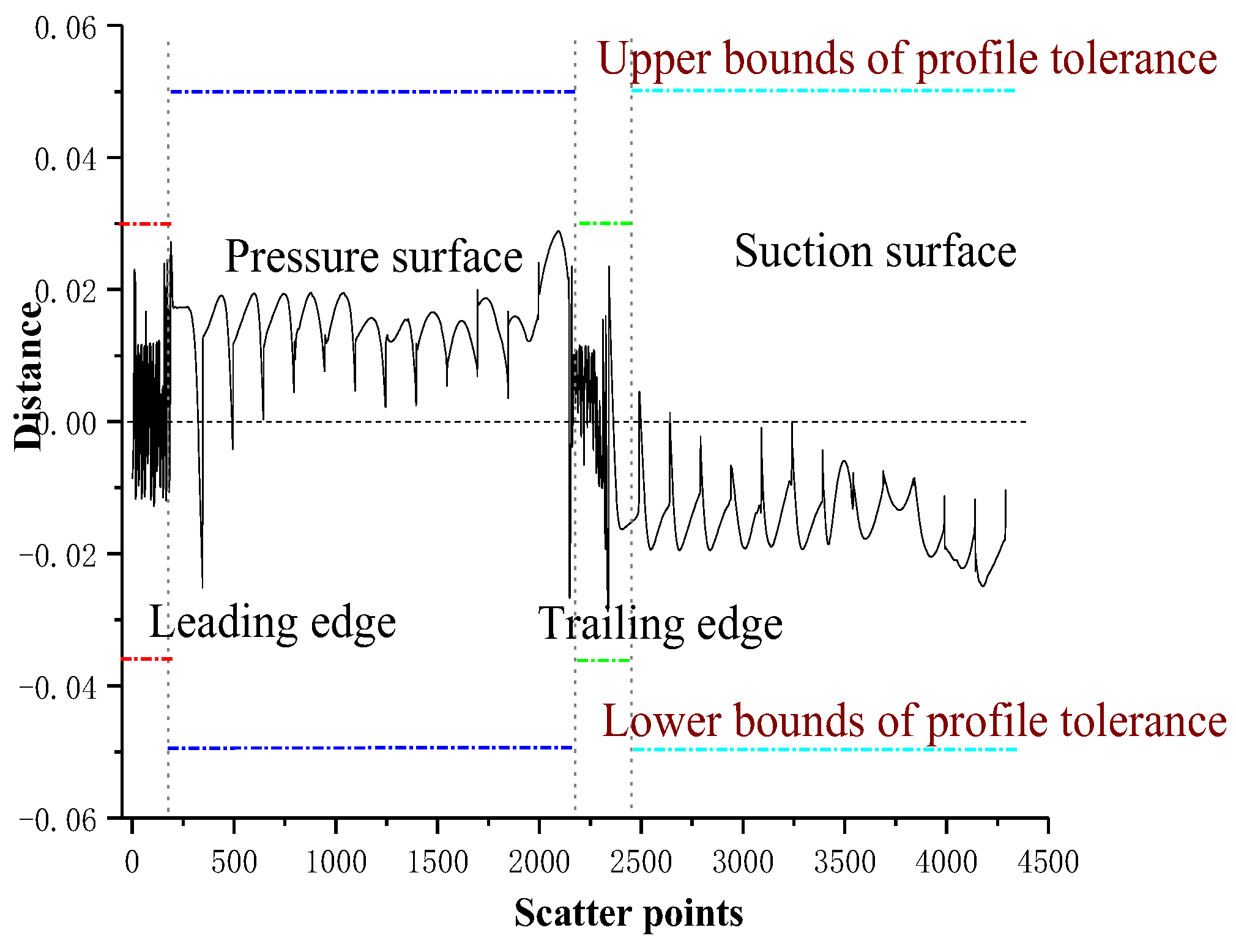
The distances between the optimized profile curves and the design profile curves for the unconstrained optimization are plotted in Figure 12. It can be observed that the profile curves were outside the profile tolerance. That is to say, the to-be-cut blade surface was not a qualified surface for generating a toolpath. Figure 13 shows the distances between the optimized profile curves and the design profile curves for the material-constraint optimization. Similarly, the to-be-cut blade surface is not a qualified surface due to the off-tolerance profile curves. The distances between the optimized profile curves and the design profile curves are plotted in Figure 14 for the multi-constraint optimization. In contrast to the results of the other two methods, they are within the profile tolerances. Thus, the to-be-cut blade surface reconstructed by the optimized profile curves is qualified.

Our results indicate that the unconstrained optimization is suitable for whole-part localization under large material allowance conditions, such as a casting and forging workpiece. Additionally, they suggest that material-constraint optimization is suitable for the to-be-cut feature under a near-net material allowance condition, such as a blend feature. Finally, the results suggest that the multi-constraint optimization is suitable for to-be-cut features under a near-net material allowance and geometric tolerance requirements.

A near-net forging blade has a free-form surface to be machined. It is a typical to-be-cut feature that has high tolerance requirements under a near-net material allowance condition. The localization method based on the multi-constraint optimization was verified to be most effective for this purpose in this experiment.

5. Conclusions

For complex surface parts such as aero-engine blades, the blade’s profile has high design precision which is usually required to meet specified profile tolerance requirements on a group of sections. However, before finish machining there are many sources of error that cause a shortage of materials on the near-net shape blade billet. If the toolpath is established according to the design blade, the machined blade may fail due to a lack of material.

The unconstrained optimization and the material-constraint optimization do not guarantee that the blade’s profile curves will be inside the profile tolerance band. To solve this problem, this paper proposed a multi-constraint optimization. By transforming the profile curves of the blade, the to-be-cut blade surface is obtained to satisfy the tolerance and material allowance requirements. Furthermore, the localization is more flexible because each profile curve has its own space transformation. The proposed method in this paper achieved improvements in satisfying the requirements of the design blade, compared to previous methods.

References

- Paul, J.B.; McKay, H.D. A Method for Registration of 3-D Shapes. IEEE Trans. Pattern Anal. Mach. Intell. 1992, 14, 239–256. [Google Scholar]
- Kang, B.; Gou, J.; Chu, Y.; Li, Z. A CAD-based probing and localisation method for arbitrarily fixed workpiece. In Proceedings of the IEEE International Conference on Robotics and Automation, Albuquerque, NM, USA, 25 April 1997; Volume 2, pp. 1259–1264. [Google Scholar]
- Chu, Y.; Gou, J.; Li, Z. On the hybrid workpiece localization/envelopment problems. In Proceedings of the IEEE International Conference on Robotics and Automation, Leuven, Belgium, 20 May 1998; Volume 4, pp. 3665–3670. [Google Scholar]
- Sun, Y.W.; Xu, J.T.; Guo, D.M.; Jia, Z.Y. A unified localization approach for machining allowance optimization of complex curved surfaces. Precis. Eng. 2009, 33, 516–523. [Google Scholar] [CrossRef]
- Mor, B.; Mosheiov, G. Parallel machine scheduling problems with common flow-allowance. Int. J. Prod. Econ. 2012, 139, 623–633. [Google Scholar] [CrossRef]
- Han, C.; Zhang, D.; Wu, B.; Pu, K.; Luo, M. Localization of freeform surface workpiece with particle swarm optimization algorithm. In Proceedings of the 2014 International Conference on Innovative Design and Manufacturing (ICIDM), Montreal, QC, Canada, 13–15 August 2014; pp. 47–52. [Google Scholar]
- Xu, J.T.; Liu, W.J.; Sun, Y.W. Optimal localization of complex surfaces in CAD-based inspection. Front. Mech. Eng. China 2008, 3, 426–433. [Google Scholar] [CrossRef] [Green Version]
- Chu, Y.X.; Gou, J.B.; Li, Z.X. Workpiece localization algorithms: Performance evaluation and reliability analysis. J. Manuf. Syst. 1999, 18, 113–126. [Google Scholar] [CrossRef]
- Li, Z.X.; Gou, J.B.; Chu, Y.X. Geometric Algorithms for Work piece Localization. IEEE Trans. Robot. Autom. 1998, 14, 864–878. [Google Scholar]
- Li, Q.D.; Riffiths, J.G.G. Iterative Closest Geometric Objects Registration. Comput. Math. Appl. 2000, 40, 1171–1183. [Google Scholar] [CrossRef] [Green Version]
- Li, W.-L.; Yin, Z.-P.; Xiong, Y.-L. Adaptive distance function and its application in free-form surface localization. In Proceedings of the 2009 International Conference on Information and Automation, Zhuhai/Macau, China, 22–24 June 2009; pp. 24–28. [Google Scholar]
- Astanin, S.; Antonelli, D.; Chiabert, P.; Alletto, C. Reflective workpiece detection and localization for flexible robotic cells. Robot. Comput. Manuf. 2017, 44, 190–198. [Google Scholar] [CrossRef]
- Sun, Y.W.; Wang, X.M.; Guo, D.M.; Liu, J. Machining localization and quality evaluation of parts with sculptured surfaces using SQP method. Int. J. Adv. Manuf. Technol. 2009, 42, 1131–1139. [Google Scholar]
- Zhang, Y.; Zhang, D.H.; Wu, B.H. An approach for machining allowance optimization of complex parts with integrated structure. J. Comput. Des. Eng. 2015, 2, 248–252. [Google Scholar] [CrossRef] [Green Version]