
Multiclassification Prediction of Clay Sensitivity Using Extreme Gradient Boosting Based on Imbalanced Dataset


Abstract
:1. Introduction
2. Materials and Methods
2.1. XGBoost
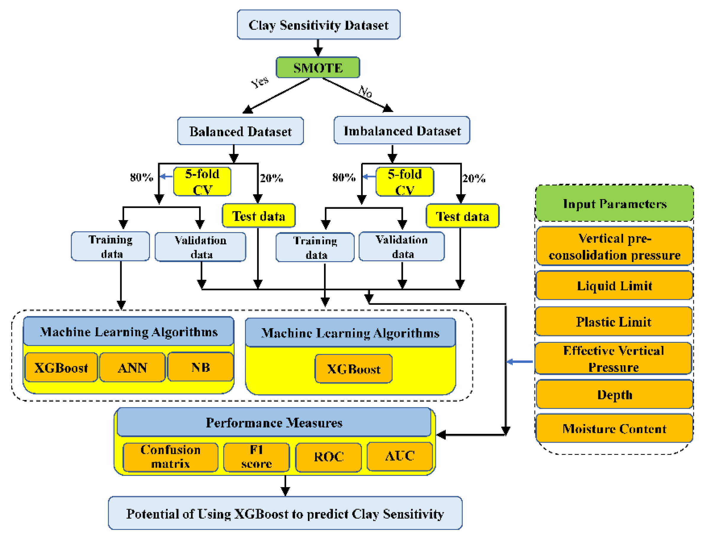
2.2. SMOTE
3. Preprocessing Data
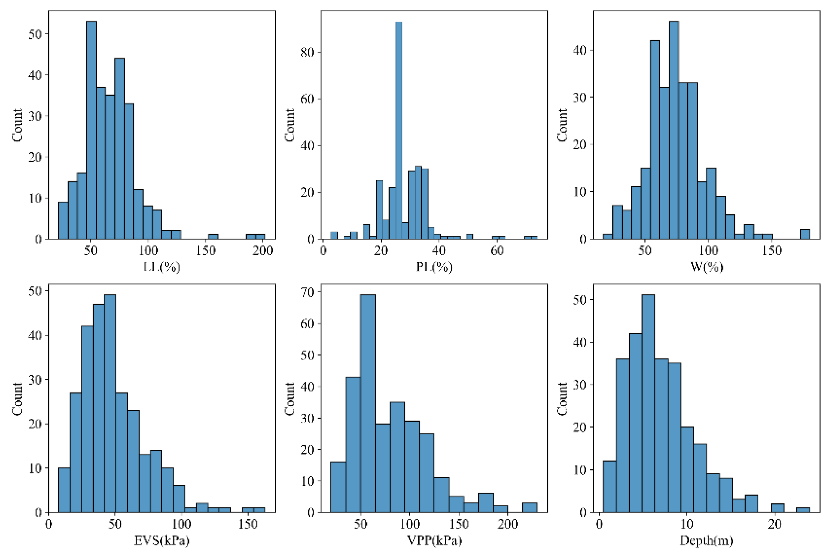
3.1. Description of Data
3.2. Data Preparation and Performance
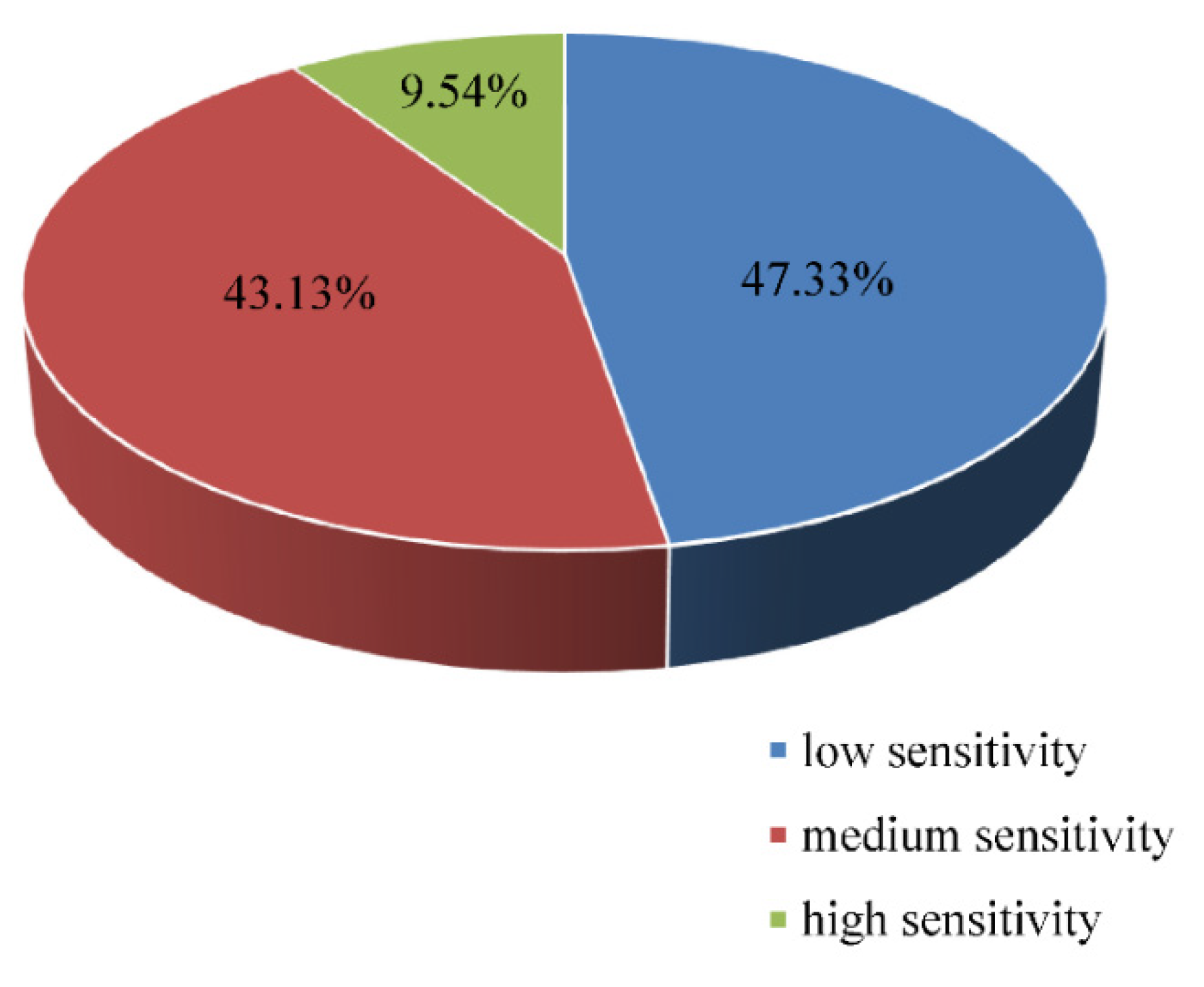
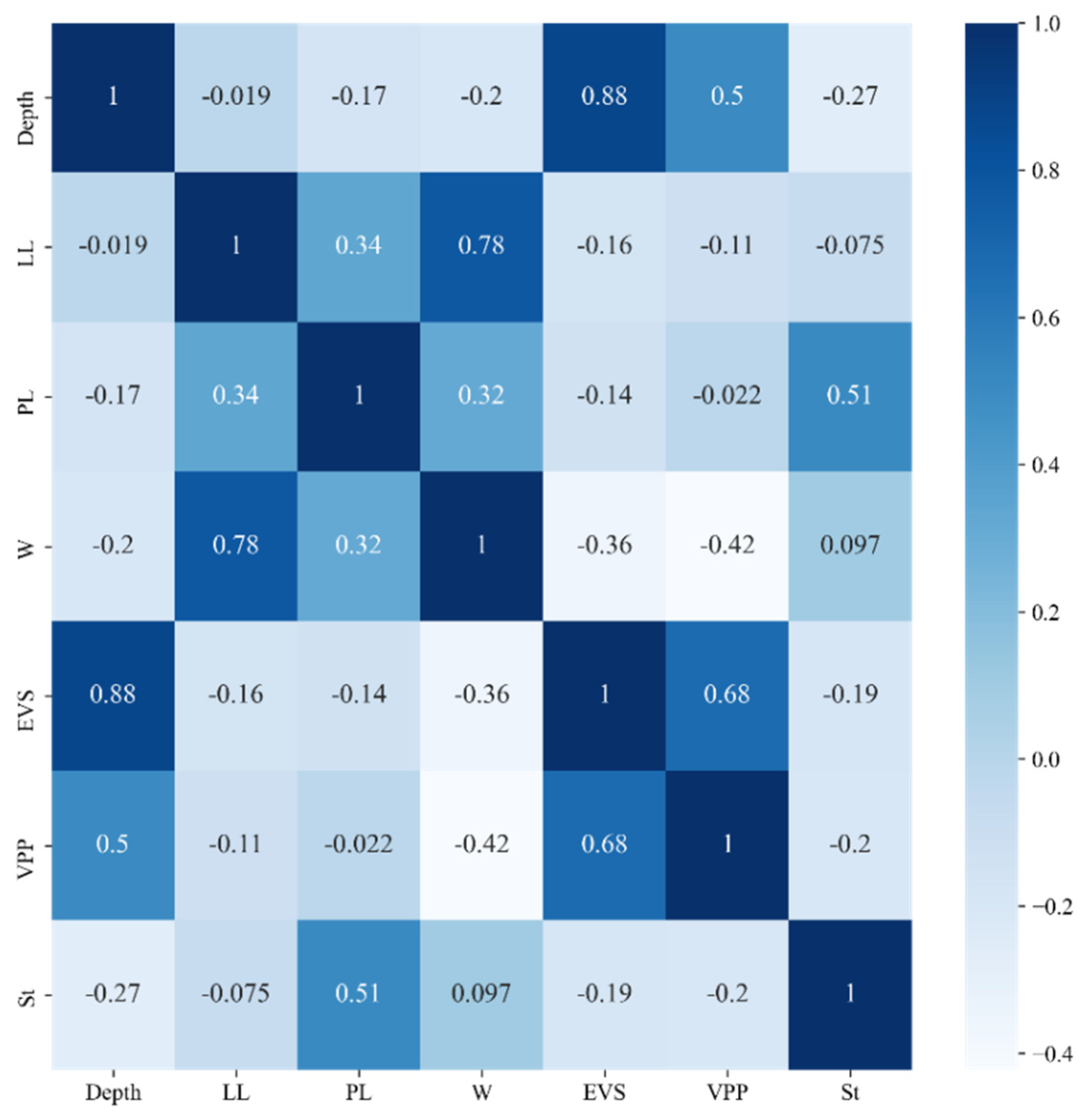
3.2.1. Analysis of Clay Dataset
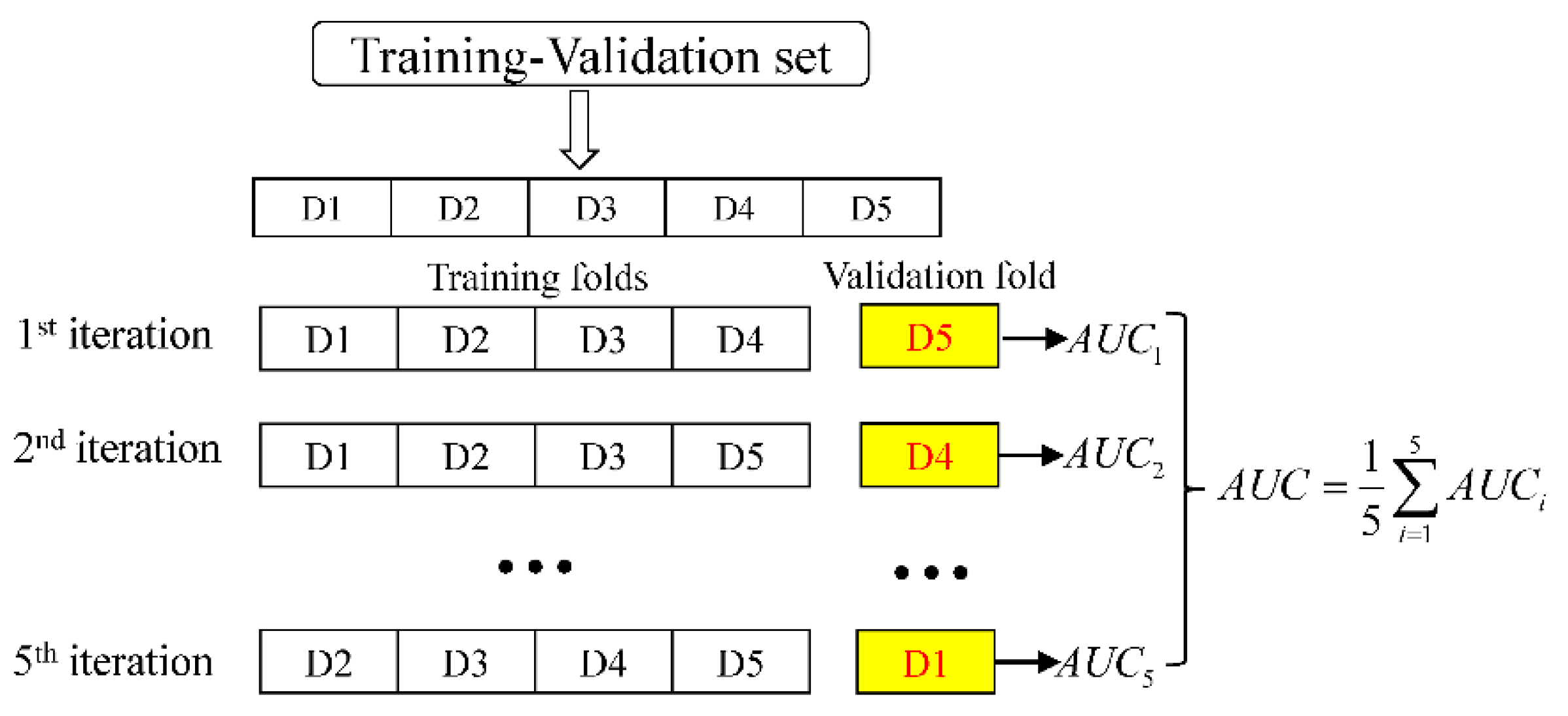
3.2.2. Cross-Validation
3.3. Performances
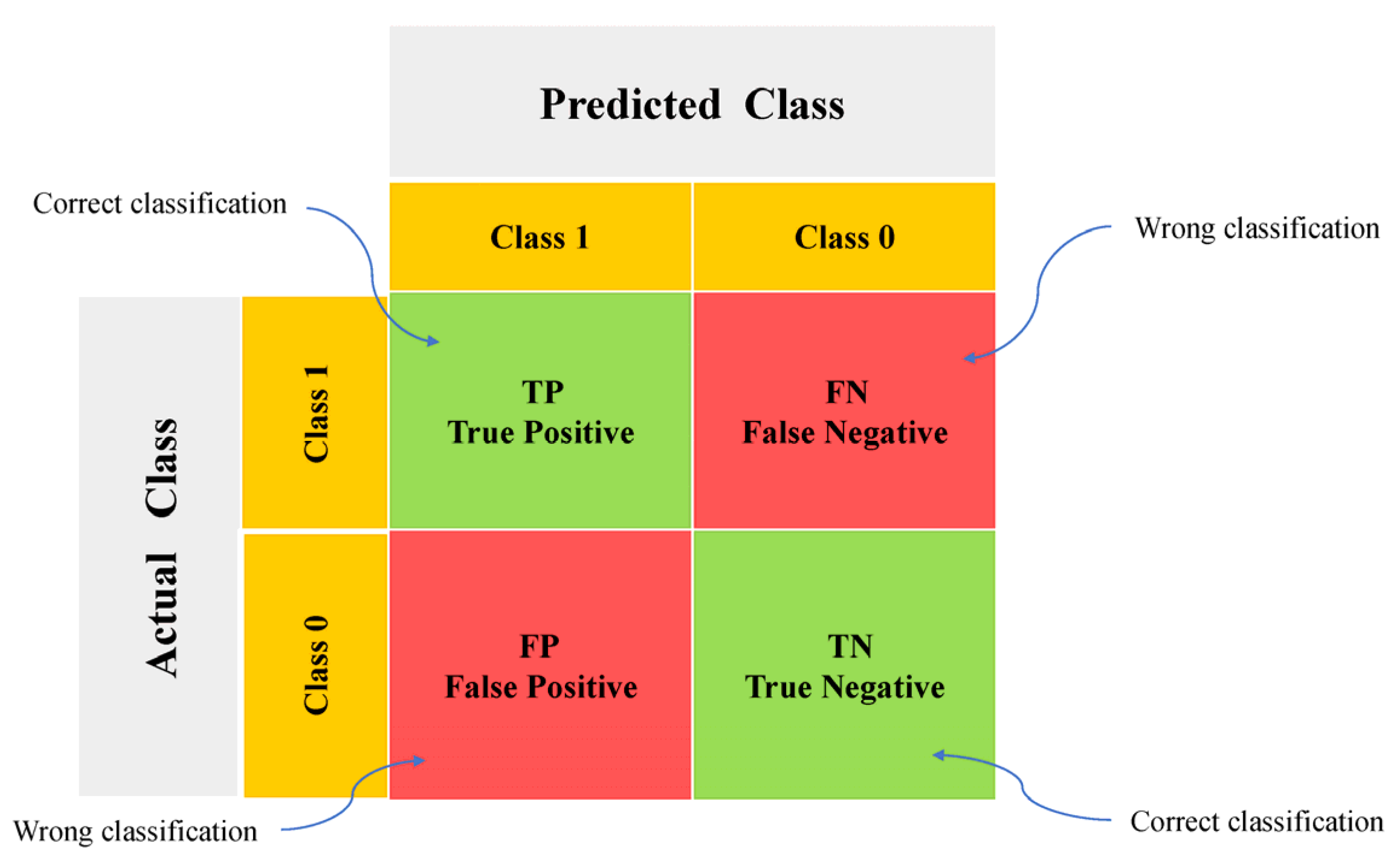
3.3.1. Confusion Matrix
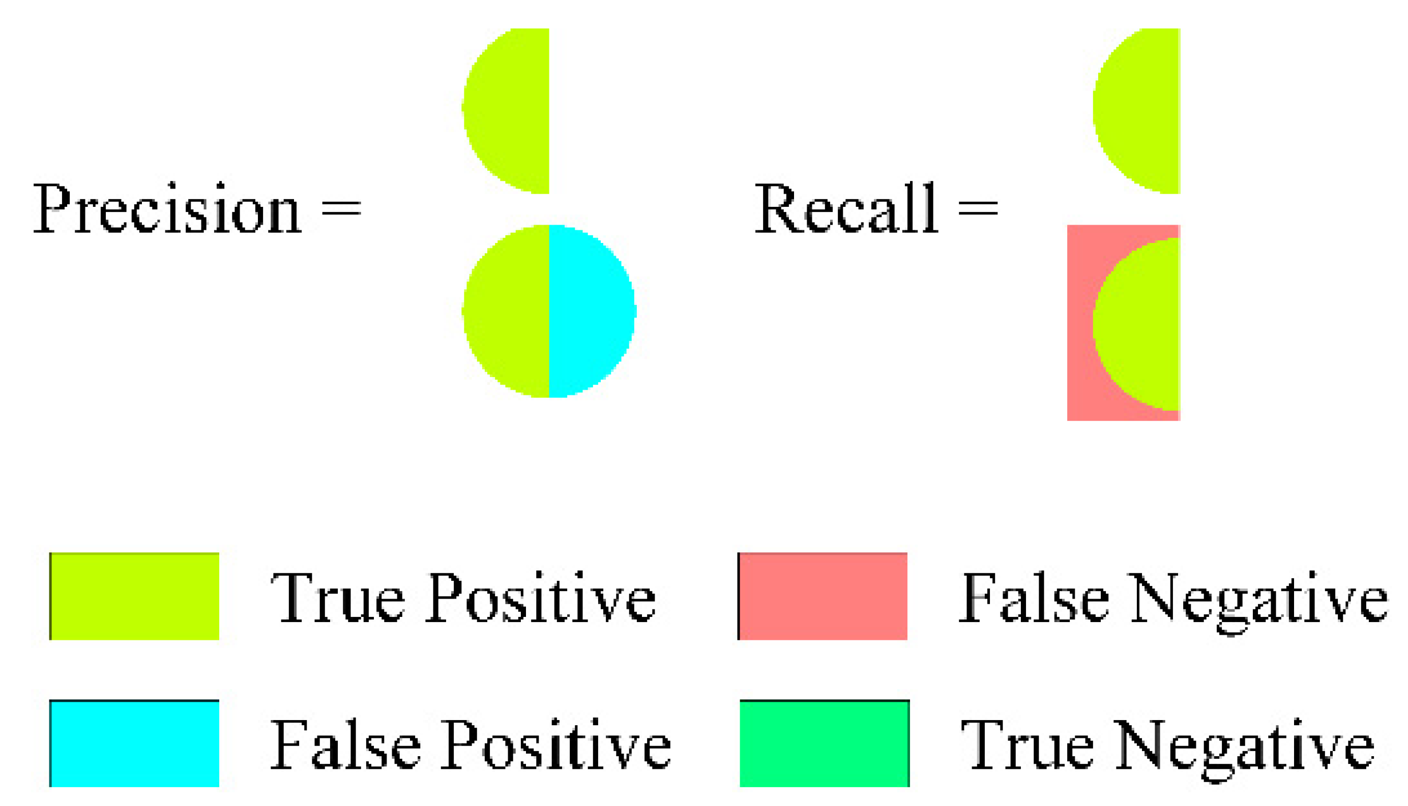
3.3.2. F1 Score
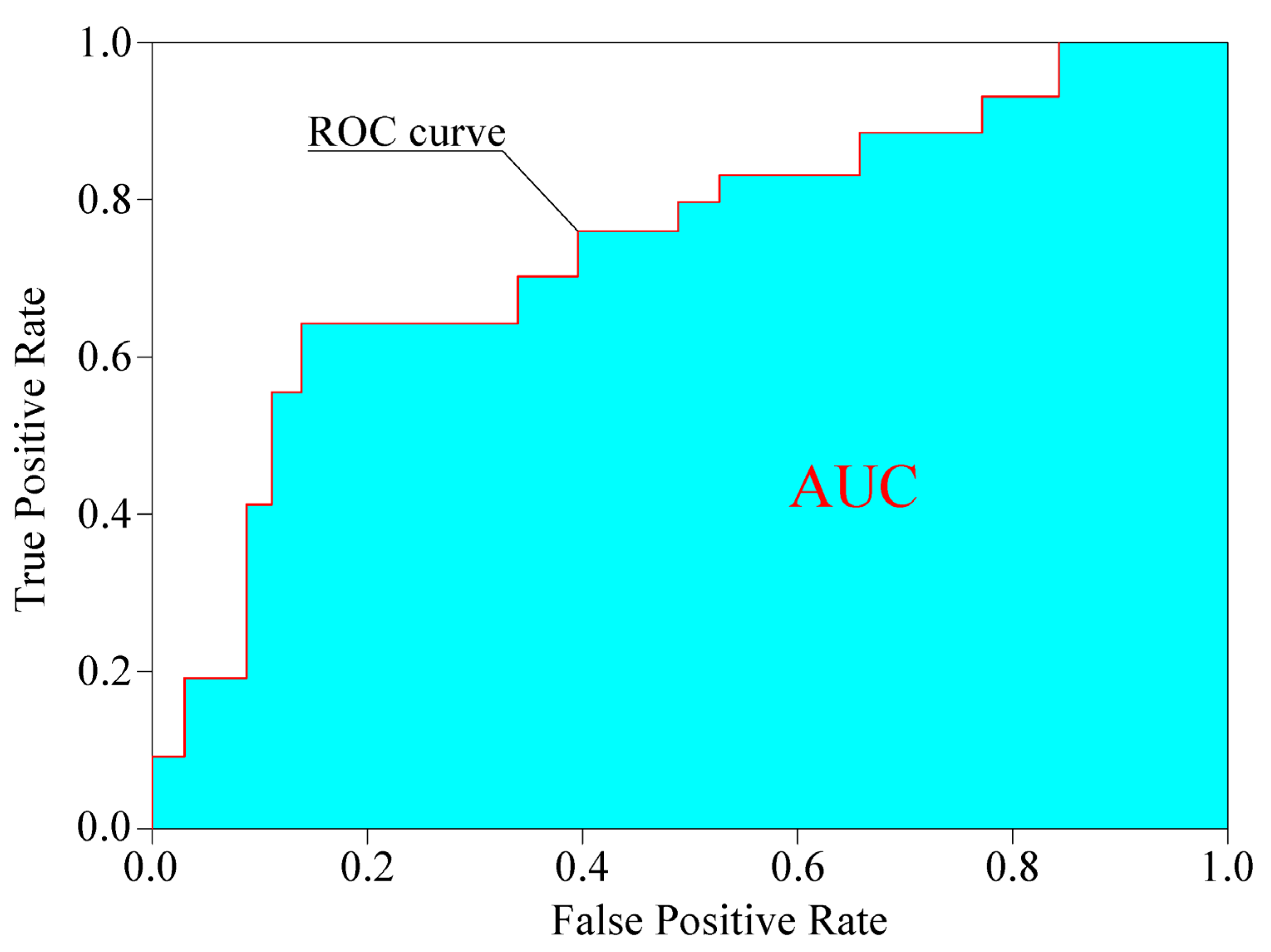
3.3.3. AUC and ROC
3.3.4. Evaluation Methods
4. Results
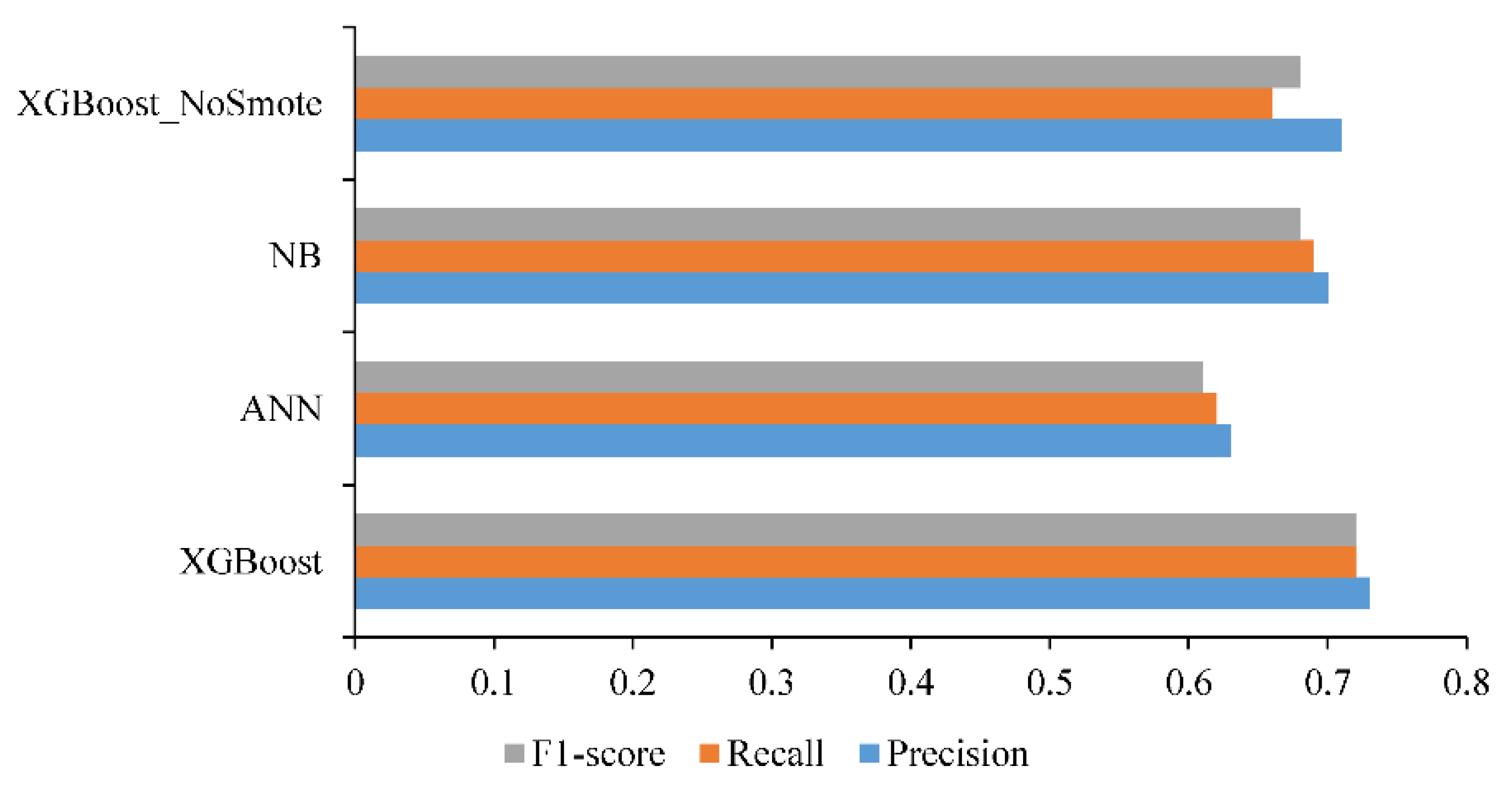
4.1. Confusion Matrix and F1 Score Results
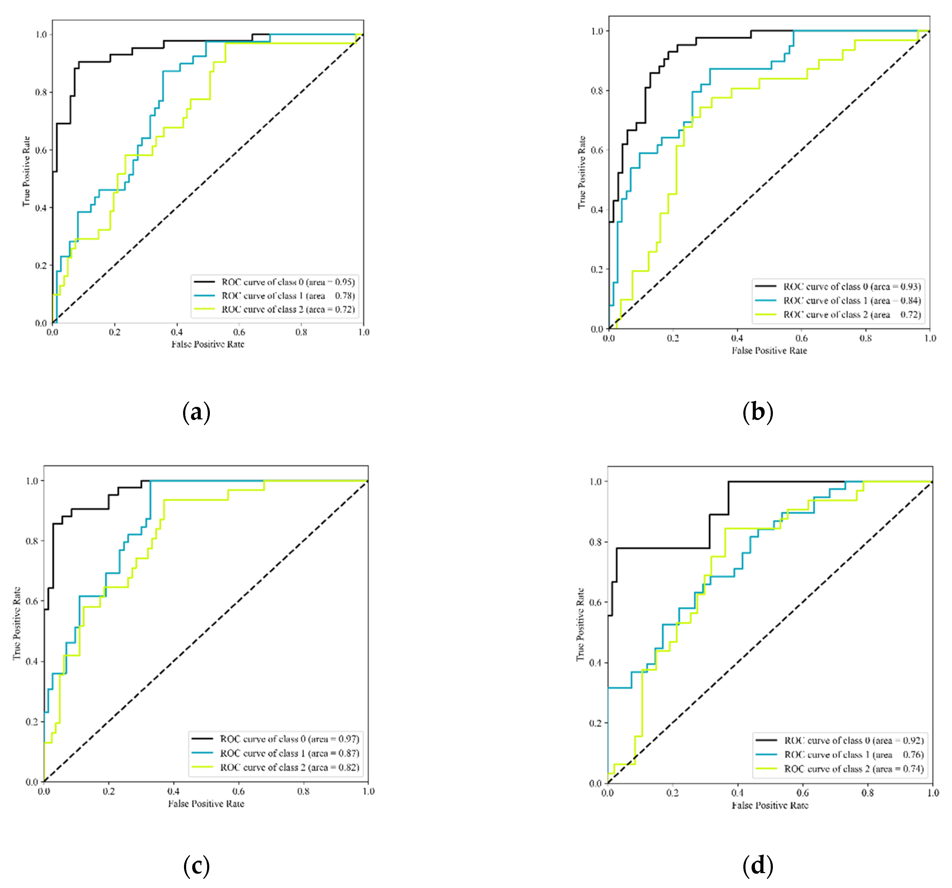
4.2. ROC and AUC Results
4.3. Compared with Previous Studies
5. Discussion
6. Conclusions
Author Contributions
Funding
Institutional Review Board Statement
Informed Consent Statement
Data Availability Statement
Conflicts of Interest
References
- Likitlersuang, S.; Surarak, C.; Wanatowski, D.; Oh, E.; Balasubramaniam, A. Finite element analysis of a deep excavation: A case study from the Bangkok MRT. Soils Found. 2013, 53, 756–773. [Google Scholar] [CrossRef] [Green Version]
- Arasan, S.; Akbulut, R.K.; Isik, F.; Bagherinia, M.; Zaimoglu, A.S. Behavior of polymer columns in soft clayey soil: A preliminary study. Geomech. Eng. 2016, 10, 95–107. [Google Scholar] [CrossRef]
- Hu, J.; Ma, F. Failure Investigation at a Collapsed Deep Open Cut Slope Excavation in Soft Clay. Geotech. Geol. Eng. 2018, 35, 665–683. [Google Scholar] [CrossRef]
- Jlassi, K.; Krupa, I.; Chehimi, M.M. Overview: Clay Preparation, Properties, Modification. Clay-Polym. Nanocomposites 2017, 1–28. [Google Scholar] [CrossRef]
- Paiva, L.B.; Morales, A.R.; Valenzuela Díaz, F.R. Organoclays: Properties, preparation and applications. Appl. Clay Sci. 2008, 42, 8–24. [Google Scholar] [CrossRef]
- Zhou, C.H.; Zhao, L.Z.; Wang, A.Q.; Chen, T.H.; He, H.P. Current fundamental and applied research into clay minerals in China. Appl. Clay Sci. 2016, 119, 3–7. [Google Scholar] [CrossRef]
- Zahid, I.; Ayoub, M.; Abdullah, B.B.; Nazir, M.H.; Zulqarnain; Kaimkhani, M.A.; Sher, F. Activation of nano kaolin clay for bio-glycerol conversion to a valuable fuel additive. Sustainability 2021, 13, 2631. [Google Scholar] [CrossRef]
- Doğan-Sağlamtimur, N.; Bilgil, A.; Szechyńska-Hebda, M.; Parzych, S.; Hebda, M. Eco-friendly fired brick produced from industrial ash and natural clay: A study of waste reuse. Materials 2021, 14, 877. [Google Scholar] [CrossRef] [PubMed]
- Otunola, B.O.; Ololade, O.O. A review on the application of clay minerals as heavy metal adsorbents for remediation purposes. Environ. Technol. Innov. 2020, 18, 100692. [Google Scholar] [CrossRef]
- Abdallah, Y.K.; Estévez, A.T. 3d-printed biodigital clay bricks. Biomimetics 2021, 6, 59. [Google Scholar] [CrossRef]
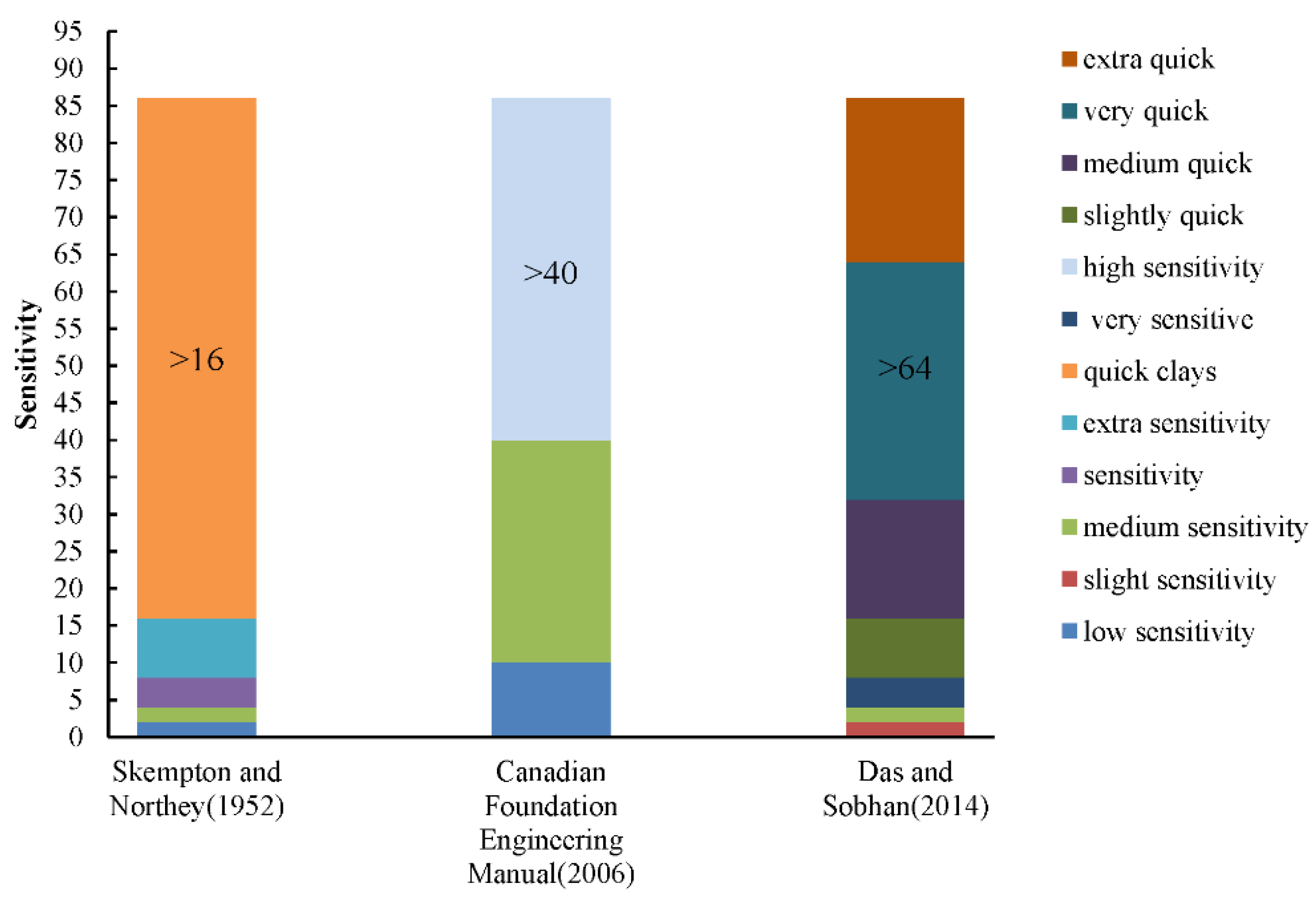
- Skempton, A.W.; Northey, R.D. The sensitivity of clays. Geotechnique 1952, 3, 30–53. [Google Scholar] [CrossRef]
- Terzaghi, K.; Peck, R.B.; Mesri, G. Soil Mechanics in Engineering Practice, 3rd ed.; John Wiley & Sons: New York, NY, USA, 2016; pp. 20–25. [Google Scholar]
- Godoy, C.; Depina, I.; Thakur, V. Application of machine learning to the identification of quick and highly sensitive clays from cone penetration tests. J. Zhejiang Univ. Sci. A 2020, 21, 445–461. [Google Scholar] [CrossRef]
- D’Ignazio, M.; Phoon, K.K.; Tan, S.A.; Länsivaara, T.T. Correlations for undrained shear strength of finish soft clays. Can. Geotech. J. 2016, 53, 1628–1645. [Google Scholar] [CrossRef] [Green Version]
- Eslami, A.; Fellenius, B.H. Pile capacity by direct CPT and CPTu methods applied to 102 case histories. Can. Geotech. J. 1997, 34, 886–904. [Google Scholar] [CrossRef]
- Gao, Y.B.; Ge, X.N. On the sensitivity of soft clay obtained by the field vane test. Geotech. Test. J. 2016, 39, 282–290. [Google Scholar] [CrossRef]
- Meijer, G.; Dijkstra, J. A novel methodology to regain sensitivity of quick clay in a geotechnical centrifuge. Can. Geotech. J. 2013, 50, 995–1000. [Google Scholar] [CrossRef]
- Schneider, J.A.; Randolph, M.F.; Mayne, P.W.; Ramsey, N.R. Analysis of Factors Influencing Soil Classification Using Normalized Piezocone Tip Resistance and Pore Pressure Parameters. J. Geotech. Geoenviron. Eng. 2008, 134, 1569–1586. [Google Scholar] [CrossRef]
- Yafrate, N.; DeJong, J.; DeGroot, D.; Randolph, M. Evaluation of Remolded Shear Strength and Sensitivity of Soft Clay Using Full-Flow Penetrometers. J. Geotech. Geoenviron. Eng. 2009, 135, 1179–1189. [Google Scholar] [CrossRef]
- Abbaszadeh Shahri, A.; Malehmir, A.; Juhlin, C. Soil classification analysis based on piezocone penetration test data-A case study from a quick-clay landslide site in southwestern Sweden. Eng. Geol. 2015, 189, 32–47. [Google Scholar] [CrossRef]
- Moreno-Maroto, J.M.; Alonso-Azcárate, J.; O’Kelly, B.C. Review and critical examination of fine-grained soil classification systems based on plasticity. Appl. Clay Sci. 2021, 200, 105955. [Google Scholar] [CrossRef]
- Robertson, P.K. Cone penetration test (CPT)-based soil behaviour type (SBT) classification system—An update. Can. Geotech. J. 2016, 53, 1910–1927. [Google Scholar] [CrossRef]
- Gylland, A.S.; Sandven, R.; Montafia, A.; Pfaffhuber, A.A.; Kåsin, K.; Long, M. Cptu classification diagrams for identification of sensitive clays. In Advances in Natural and Technological Hazards Research; Springer: Cham, Switzerland, 2017. [Google Scholar]
- Zhang, W.; Wu, C.; Li, Y.; Wang, L.; Samui, P. Assessment of pile drivability using random forest regression and multivariate adaptive regression splines. Georisk 2021, 15, 27–40. [Google Scholar] [CrossRef]
- Dickson, M.E.; Perry, G.L.W. Identifying the controls on coastal cliff landslides using machine-learning approaches. Environ. Model. Softw. 2016, 76, 117–127. [Google Scholar] [CrossRef]
- Pourghasemi, H.R.; Rahmati, O. Prediction of the landslide susceptibility: Which algorithm, which precision? Catena 2018, 162, 177–192. [Google Scholar] [CrossRef]
- Li, S.H.; Wu, L.Z.; Luo, X.H. A novel method for locating the critical slip surface of a soil slope. Eng. Appl. Artif. Intell. 2020, 94, 103733. [Google Scholar] [CrossRef]
- Zhu, S.; Wu, L.; Huang, J. Application of an improved P(m)-SOR iteration method for flow in partially saturated soils. Comput. Geosci. 2021, 1–15. [Google Scholar] [CrossRef]
- Pham, B.T.; Son, L.H.; Hoang, T.A.; Nguyen, D.M.; Tien Bui, D. Prediction of shear strength of soft soil using machine learning methods. Catena 2018, 166, 181–191. [Google Scholar] [CrossRef]
- Mishra, P.; Samui, P.; Mahmoudi, E. Probabilistic design of retaining wall using machine learning methods. Appl. Sci. 2021, 11, 5411. [Google Scholar] [CrossRef]
- Huang, Z.; Zhang, D.; Zhang, D. Application of ANN in Predicting the Cantilever Wall Deflection in Undrained Clay. Appl. Sci. 2021, 11, 9760. [Google Scholar] [CrossRef]
- Li, S.H.; Luo, X.H.; Wu, L.Z. A new method for calculating failure probability of landslide based on ANN and a convex set model. Landslides 2021, 18, 2855–2867. [Google Scholar] [CrossRef]
- Wu, L.Z.; Li, S.H.; Huang, R.Q.; Xu, Q. A new grey prediction model and its application to predicting landslide displacement. Appl. Soft Comput. J. 2020, 95, 106543. [Google Scholar] [CrossRef]
- Zhang, W.; Wu, C.; Zhong, H.; Li, Y.; Wang, L. Prediction of undrained shear strength using extreme gradient boosting and random forest based on Bayesian optimization. Geosci. Front. 2021, 12, 469–477. [Google Scholar] [CrossRef]
- Chen, R.P.; Li, Z.C.; Chen, Y.M.; Ou, C.Y.; Hu, Q.; Rao, M. Failure Investigation at a Collapsed Deep Excavation in Very Sen-sitive Organic Soft Clay. J. Perform. Constr. Facil. 2015, 29, 04014078. [Google Scholar] [CrossRef]
- Gylland, A.; Long, M.; Emdal, A.; Sandven, R. Characterisation and engineering properties of Tiller clay. Eng. Geol. 2013, 164, 86–100. [Google Scholar] [CrossRef] [Green Version]
- Abbaszadeh Shahri, A. An Optimized Artificial Neural Network Structure to Predict Clay Sensitivity in a High Landslide Prone Area Using Piezocone Penetration Test (CPTu) Data: A Case Study in Southwest of Sweden. Geotech. Geol. Eng. 2016, 34, 86–100. [Google Scholar] [CrossRef]
- Canadian Foundation Engineering Manual, 4th ed.; Canadian Geotechnical Society: Prince George, BC, Canada, 2006; pp. 17–20.
- Das, B.; Sobhan, K. Principles of Geotechnical Engineering, 8th ed.; CENGAGE Learning: Stanford, CA, USA, 2014; pp. 450–466. [Google Scholar]
- Chawla, N.V.; Bowyer, K.W.; Hall, L.O.; Kegelmeyer, W.P. SMOTE: Synthetic minority over-sampling technique. J. Artif. Intell. Res. 2002, 16, 321–357. [Google Scholar] [CrossRef]
- Liu, Q.; Wang, X.; Huang, X.; Yin, X. Prediction model of rock mass class using classification and regression tree integrated AdaBoost algorithm based on TBM driving data. Tunn. Undergr. Sp. Technol. 2020, 106, 103595. [Google Scholar] [CrossRef]
- Chen, T.; Guestrin, C. XGBoost: A scalable tree boosting system. In Proceedings of the ACM SIGKDD International Conference on Knowledge Discovery and Data Mining, San Francisco, CA, USA, 13–17 August 2016. [Google Scholar] [CrossRef] [Green Version]
- Japkowicz, N. The Class Imbalance Problem: Significance and Strategies. In Proceedings of the 2000 International Conference on Artificial Intelligence, Acapulco, Mexico, 11–14 April 2000. [Google Scholar]
- Ching, J.; Phoon, K.K. Transformations and correlations among some clay parameters-The global database. Can. Geotech. J. 2014, 51, 663–685. [Google Scholar] [CrossRef]
- Pedregosa, F.; Varoquaux, G.; Gramfort, A.; Michel, V.; Thirion, B.; Grisel, O.; Blondel, M.; Prettenhofer, P.; Weiss, R.; Du-bourg, V.; et al. Scikit-learn: Machine learning in Python. J. Mach. Learn. Res. 2011, 12, 2825–2830. [Google Scholar]
- Alkroosh, I.; Nikraz, H. Predicting axial capacity of driven piles in cohesive soils using intelligent computing. Eng. Appl. Artif. Intell. 2012, 25, 618–627. [Google Scholar] [CrossRef]
- Kohavi, R. A Study of Cross-Validation and Bootstrap for Accuracy Estimation and Model Selection. Int. Jt. Conf. Artif. Intell. 1995, 14, 1137–1145. [Google Scholar]
- Wong, T.T. Performance evaluation of classification algorithms by k-fold and leave-one-out cross validation. Pattern Recognit. 2015, 48, 2839–2846. [Google Scholar] [CrossRef]
- Trajdos, P.; Kurzynski, M. Weighting scheme for a pairwise multi-label classifier based on the fuzzy confusion matrix. Pattern Recognit. Lett. 2018, 103, 60–67. [Google Scholar] [CrossRef] [Green Version]
- Xue, Y.; Bai, C.; Qiu, D.; Kong, F.; Li, Z. Predicting rockburst with database using particle swarm optimization and extreme learning machine. Tunn. Undergr. Sp. Technol. 2020, 98, 103287. [Google Scholar] [CrossRef]
- Fawcett, T. An introduction to ROC analysis. Pattern Recognit. Lett. 2006, 27, 861–874. [Google Scholar] [CrossRef]
- Huang, J.; Ling, C.X. Using AUC and accuracy in evaluating learning algorithms. IEEE Trans. Knowl. Data Eng. 2005, 17, 299–310. [Google Scholar] [CrossRef] [Green Version]
- Pei, L.; Sun, Z.; Yu, T.; Li, W.; Hao, X.; Hu, Y.; Yang, C. Pavement aggregate shape classification based on extreme gradient boosting. Constr. Build. Mater. 2020, 256, 119356. [Google Scholar] [CrossRef]
- García, V.; Mollineda, R.A.; Sánchez, J.S. On the k-NN performance in a challenging scenario of imbalance and overlapping. Pattern Anal. Appl. 2008, 11, 269–280. [Google Scholar] [CrossRef]
- López, V.; Fernández, A.; García, S.; Palade, V.; Herrera, F. An insight into classification with imbalanced data: Empirical re-sults and current trends on using data intrinsic characteristics. Inf. Sci. 2013, 250, 113–141. [Google Scholar] [CrossRef]


| Depth (m) | LL (%) | PL (%) | W (%) | EVS (kPa) | VPP (kPa) | St | |
|---|---|---|---|---|---|---|---|
| mean | 6.97 | 68.37 | 28.49 | 76.47 | 48.72 | 79.82 | 16.27 |
| std | 3.95 | 23.86 | 7.97 | 23.32 | 27.33 | 48.54 | 13.26 |
| min | 0.50 | 22.00 | 2.73 | 17.27 | 6.86 | 15.2 | 2.00 |
| 50% | 6.00 | 68.72 | 27.02 | 75.00 | 43.08 | 64.88 | 11.00 |
| max | 24.00 | 201.81 | 73.92 | 180.11 | 212.87 | 315.64 | 64.00 |
| Model | Parameters | Value |
|---|---|---|
| XGBoost | n_estimators | 360 |
| learning_rate | 0.002 | |
| max_depth | 6 | |
| min_child_weight | 1 | |
| gamma | 0.2 | |
| colsample_bytree | 0.5 | |
| subsample | 0.8 | |
| ANN | learning_rate_init | 0.0001 |
| activation | tanh | |
| hidden_layer_sizes | (100, 100, 100) | |
| max_iter | 260 | |
| NB | priors | 3 |
| var_smoothing | 10−9 | |
| XGBoost_NoSmote | n_estimators | 360 |
| learning_rate | 0.005 | |
| max_depth | 5 | |
| min_child_weight | 1 | |
| gamma | 0.3 | |
| colsample_bytree | 0.7 | |
| subsample | 0.8 |
| Evaluation Measures | Models | |||
| XGBoost | ANN | NB | XGBoost_NoSmote | |
| Precision | 0.73 | 0.63 | 0.70 | 0.71 |
| Recall | 0.72 | 0.62 | 0.69 | 0.66 |
| F1 score | 0.72 | 0.61 | 0.68 | 0.68 |
| AUC of high sensitivity | 0.97 | 0.95 | 0.93 | 0.92 |
| AUC of medium sensitivity | 0.82 | 0.72 | 0.72 | 0.74 |
| AUC of low sensitivity | 0.87 | 0.78 | 0.84 | 0.76 |
| Mean AUC of classification | 0.89 | 0.82 | 0.83 | 0.81 |
Publisher’s Note: MDPI stays neutral with regard to jurisdictional claims in published maps and institutional affiliations. |
© 2022 by the authors. Licensee MDPI, Basel, Switzerland. This article is an open access article distributed under the terms and conditions of the Creative Commons Attribution (CC BY) license (https://creativecommons.org/licenses/by/4.0/).
Share and Cite
Ma, T.; Wu, L.; Zhu, S.; Zhu, H. Multiclassification Prediction of Clay Sensitivity Using Extreme Gradient Boosting Based on Imbalanced Dataset. Appl. Sci. 2022, 12, 1143. https://doi.org/10.3390/app12031143
Ma T, Wu L, Zhu S, Zhu H. Multiclassification Prediction of Clay Sensitivity Using Extreme Gradient Boosting Based on Imbalanced Dataset. Applied Sciences. 2022; 12(3):1143. https://doi.org/10.3390/app12031143
Chicago/Turabian StyleMa, Tao, Lizhou Wu, Shuairun Zhu, and Hongzhou Zhu. 2022. "Multiclassification Prediction of Clay Sensitivity Using Extreme Gradient Boosting Based on Imbalanced Dataset" Applied Sciences 12, no. 3: 1143. https://doi.org/10.3390/app12031143