Reducing False Negatives in Ransomware Detection: A Critical Evaluation of Machine Learning Algorithms

Abstract

Technological achievement and cybercriminal methodology are two parallel growing paths; protocols such as Tor and i2p (designed to offer confidentiality and anonymity) are being utilised to run ransomware companies operating under a Ransomware as a Service (RaaS) model. RaaS enables criminals with a limited technical ability to launch ransomware attacks. Several recent high-profile cases, such as the Colonial Pipeline attack and JBS Foods, involved forcing companies to pay enormous amounts of ransom money, indicating the difficulty for organisations of recovering from these attacks using traditional means, such as restoring backup systems. Hence, this is the benefit of intelligent early ransomware detection and eradication. This study offers a critical review of the literature on how we can use state-of-the-art machine learning (ML) models to detect ransomware. However, the results uncovered a tendency of previous works to report precision while overlooking the importance of other values in the confusion matrices, such as false negatives. Therefore, we also contribute a critical evaluation of ML models using a dataset of 730 malware and 735 benign samples to evaluate their suitability to mitigate ransomware at different stages of a detection system architecture and what that means in terms of cost. For example, the results have shown that an Artificial Neural Network (ANN) model will be the most suitable as it achieves the highest precision of 98.65%, a Youden’s index of 0.94, and a net benefit of 76.27%, however, the Random Forest model (lower precision of 92.73%) offered the benefit of having the lowest false-negative rate (0.00%). The risk of a false negative in this type of system is comparable to the unpredictable but typically large cost of ransomware infection, in comparison with the more predictable cost of the resources needed to filter false positives.

1. Introduction

Ransomware is malicious software that prevents users from accessing their data until a ransom payment is made, usually in Bitcoins. It broadly falls into two main categories: locker ransomware, which prevents access to computers, and crypto-ransomware, which encrypts user files such as databases, documents, spreadsheets, and pictures, rendering them unusable until the ransom is paid and the decryption key is obtained [1]. Ransomware malware is commonly distributed by links and attachments in spam and phishing emails [2]. It is not a new phenomenon. The first ransomware appeared in 1989 with the AIDS Trojan, and the first modern type, GPCoder, was released in 2005 [3]. Early versions of that type of threat demanded payment in the form of pre-paid bank cards or having the victim call a premium rate phone number. The advent of crypto-currencies has made anonymous payment methods possible. Mimecast reported that 61% of organisations suffered a business-disrupting ransomware attack in 2020, compared to 51% in the preceding year [4].

From an attacker’s perspective, ransomware is attractive due to its low risk and lucrative nature. Although Bitcoin wallet addresses are publicly available, wallets cannot usually be traced to specific individuals or groups [5]. At the same time, it is a lucrative crime because there has been a shift towards targeting organisations that can afford to pay, as in the case of the Colonial Pipeline, which paid a ransom of $4.4 m [6] and the meat supplier JBS, who paid a ransom of $11 m [7]. Organisations that are likely to pay to avoid risk to life are also common targets, as in the case of the Hollywood Presbyterian Medical Center [8]. Governmental and non-profit organisations are increasingly being targeted [9], and there is evidence of increased ransomware attacks against educational institutions [10].

The lucrative nature of ransomware has led to the development of Ransomware as a Service (RaaS) [11]. Criminal groups such as Darkside and Revil, who have the technical ability to conduct ransomware attacks, make their services available on the darknet, taking a percentage of the ransom as their payment. As a result, it is now possible for criminals with limited technical ability to launch ransomware attacks [12].

In most cases, ransomware is triggered by users clicking a link in a malicious email [13]. Such emails may be common spam, or they may be more sophisticated. Phishing emails attempt to trick the recipient into opening a malicious attachment by mimicking the appearance of a legitimate email. Spear-phishing emails are targeted at a specific individual or organisation, while Whale-phishing emails are aimed at senior employees who have greater access to sensitive information and authority to make payments than regular employees.

Other delivery methods include exploit kits, which take advantage of unpatched vulnerabilities in operating systems and browsers to spread malware or pivot through the network to hide the origin of the attack [14], and malvertising—when attackers create adverts containing malicious code, then serve from a legitimate ad network. Microsoft Office Macros—Visual Basic for Applications (VBA) is a comprehensive language containing commands that can be used maliciously or to download and execute other malware.

Finally, there is RDP—as Microsoft’s Remote Desktop Protocol uses port 3389 by default, attackers can scan for networks in which port 3389 is open and attempt to gain access by either brute-forcing the credentials or gaining credentials using phishing techniques.

New ransomware variants are continually emerging, and variants within the same family often employ obfuscation to evade detection by traditional methods [15,16]. A different approach to ransomware detection is therefore required, for example, to overcome the limitation of signature-based detection [15].

Machine learning (ML) offers a smarter opportunity to detect ransomware based on its behaviour, but this approach is often narrowly focused. Hence, ML models may miss cyber threats they have not seen before. The reliability of these models is determined by error parameters in which accurate predictions mean fewer false positives and fewer false negatives. However, we observe a tendency of previous works to focus on accuracy and overlook the importance of other values, such as false negatives [17]. False negatives are a crucial error parameter yielded that could be very costly to the environment. Hence, this study offers a comprehensive critical evaluation of ML models using several matrices to achieve specific efficiency targets, including but not limited to the design of an ML-based ransomware detection architecture with fewer false negatives.

This study analysed the API calls made by a range of ransomware samples and non-malicious software (730 ransomware and 735 benign samples). This has enabled the creation of a dataset that does not exhibit class imbalance and is used to train and evaluate a range of machine-learning models for detecting ransomware. The machine learning models tested are the Support Vector Machine, K-Nearest Neighbours, Logistic Regression, Decision Tree, Random Forest, and Artificial Neural Network. In addition to the metrics commonly used for the evaluation, the metrics proposed by Kok et al. [17]. have been calculated, and their usefulness in comparing the models has been evaluated. Nonetheless, our methodology demonstrates an approach to storing API call usage statistics in a relational database management system, which allows new datasets to be rapidly and flexibly created. This study has enabled us to address the following two key research questions: (1) which error parameters and evaluation matrices should be utilised by the state-of-the-art to discuss the reliability of ML models for the detection of ransomware, and (2) which ML models offer reliability for the detection of ransomware?

In the remaining part of this paper, we cover the background and related work in Section 2 and a gap analysis indicating the areas that may currently be under research. Section 3 describes the proposed architecture and emulator environment used to analyse the ransomware and benign samples, and the dataset preparation, including a short description of the machine learning algorithms. The evaluation metrics used to examine the performance of the ML models are discussed in Section 4, while Section 5 discusses the main results and analysis from our experiments and Section 6 concludes our work.

2. Background

Cybercriminals can spread ransomware by exploiting the Remote Desktop Protocol (RDP), a communications protocol that can access another computer over a network connection. As a defensive method, Convolutional Neural Networks (CNN) can be used within Intrusion Detection Systems (IDS), which monitor the network traffic and the Quality of Service or bandwidth-throttling, and can potentially identify anomalies, including security and operational issues [18]. Some traffic can be identified from the ports used (e.g., HTTP on port 80), some from non-standard ports, and some is generated by web applications that operate on dynamically-selected ports above 1024. In a review of ransomware detection approaches, Aslan et al. [15] explain why signature-based detection is efficient at reducing false negatives but is less effective on more complex malware that may employ obfuscation techniques such as encryption, oligomorphic, and polymorphic codes. Among others, this research presents a range of detection techniques, including ‘Behaviour’, ‘Heuristic’, ‘Model-checking’, and ‘Deep learning-based detection’. Moreover, they categorised the cloud and mobile device-based detection methods differently as this category is distinguished by the location where detection occurs rather than the method.

Moreira et al. [19] presented a behavioural feature analysis of ransomware during the destruction phase in Windows OS. Their approach was first to categorise the APIs based on Microsoft naming conventions (merging different API versions with similar names), then eliminate features with low variances and investigate the attacks’ behaviour. With the use of Naive Bayes (NB), K-Nearest Neighbors (KNN), Logistic Regression (LR), Random Forest (RF), Stochastic Gradient Descent (SGD), and Support Vector Machine (SVM) classification algorithms, they identified behavioural pattern modifications between ransomware and goodware. APIs’ most significant behavioural characteristics involve handling thread/process manipulation, physical memory operations, computer identification, and file type discovery operations. In contrast, the goodware presented virtual memory, files, directories, and resource operations, including DLLs.

Netto et al. [20] present a method of detecting ransomware using static and dynamic analysis. Their static analysis approach consists of two elements. The first involves the creation of randomly named ‘honey trap’ files scattered throughout the file system. These files have a ‘trigger’ attached which fires when the file is altered. Although the mechanism for this trigger is not fully described, methods to provide the needed output are available from classes such as the FileSystemWatcher class. When one of the honeypot files is modified, ransomware is assumed responsible for the modification, alerting the user. However, this approach has some problems. Creating the honey trap files at system start-up can take considerable time (several hours) for a terabyte filesystem. By the time a honey trap file is modified and the alert raised, many user files might already have been encrypted, as the tool does not stop the ransomware from continuing to execute and only alerts the user. Moreover, events can be missed when the buffer size is exceeded (e.g., by the FileSystemWatcher class) or when monitoring files with long names [21]. The second element is based on analysing the source and destination IPs and ports of packets entering and leaving the user’s system. These packets are compared with a dataset, and if a match is found, then the packet is dropped, and the remote IP is blacklisted. This approach is very similar to signature-based detection, which requires preparing and regularly updating a signature dataset. On the other side, this technique is not generally considered appropriate for reducing false negatives due to the frequent changes in code and behaviour exhibited by ransomware. The second element, the dynamic approach, involves the inspection of network packets for ‘known hexadecimal for properties’, including registry and file operations, and comparison against a pre-existing dataset. The packet is dropped if a match is found, and a Windows firewall rule is added to prevent further traffic to/from the related IP. This approach also appears to be very similar to signature-based detection, with the associated limitations.

Anand et al. [22] collected a list of 135 API calls based on a dynamic analysis by combining static and dynamic feature sets such as AvosLocker, LockBit2.0, Babuk, Hive, Conti, and Stop Ransomware and focusing on their behavioural patterns. The 135 API call analysis was used to build a machine learning model to assist security experts in detecting and blocking malicious processes at runtime. With the Adaboost Algorithm, they could classify the unseen samples with an accuracy of 0.9769 and a specificity value of 0.9508. Based on the authors’ opinion, further investigation and tests need to be performed concerning intermittent ransomware encryption and the rate at which the encryption is delivered.

Kok et al. [17] describe shortcomings with the metrics commonly used to measure the effectiveness of machine learning-based uncaught threat detection methods. Their criticism of widely used metrics is based on the fact that, with the exception of accuracy, they do not take into account the values of all four quadrants of the Confusion Matrix—True Positive, False Positive, True Negative, and False Negative. Instead, new metrics (Likelihood Ratio, Diagnostic Odds Ratio, Number Needed to Diagnose, Number Needed to Misdiagnose, and Net Benefit) are proposed, with formulae for calculating each one of them.

Bae et al. [23] have presented a machine-learning method for detecting ransomware by analysing Windows API calls. The file-related I/O calls made by sample executables (300 benign, 1000 ransomware, and 900 malware) were extracted using the Intel PIN tool [24]. Since malicious software usually uses a sequence of API calls to perform a malicious action (rarely a single API call), n-grams of API calls were generated with n values ranging from 1 to 4. The researchers found that n = 4 gave the best results; values of n equal to or larger than 4 were not investigated due to the computational difficulty. The datasets produced were used to train six algorithms—Random Forest, Logistic Regression, Naïve Bayes, Stochastic Gradient Descent, K-Nearest Neighbours, and Support Vector Machine. Testing results have shown high accuracy in detecting ransomware using this method. According to [23], the presented method of extracting the API sequences using n-gram techniques was successfully tested for detecting known and unknown ransomware, among other malware types.

Ahmed et al. [25] assumed that the analysis of system calls is the most widely used approach for detecting ransomware attacks and that ransomware authors often inject irrelevant system calls to generate ‘noise’ and make the sequence of calls more challenging to analyse. They propose a filtering method based on mRmR (Maximum-Relevance Minimum-Redundancy) known as EmRmR (Enhance Maximum-Relevance and Minimum-Redundancy) to eliminate noise and select the most relevant features. EmRmR is less computationally expensive than mRmR and, thus, more suitable for ransomware detection.

Sheen’s and Yadav’s [26] method of ransomware detection is based on the static analysis of executables. They note that certain API calls are used more frequently in ransomware than in non-malicious executables. The API calls made by 16,243 ransomware samples and 3620 non-malicious executables were analysed using the Radare2 disassembler. They describe the potential for problems introduced by ‘class imbalance’ resulting from a large number of ransomware samples compared to benign samples and their use of the Synthetic Minority Oversampling Technique (SMOTE) to synthesise further benign samples [27]. API calls that occurred more frequently in ransomware than benign executables were selected, resulting in a dataset of 160 features. These features were used to train models using a variety of machine-learning algorithms, which were then evaluated. The paper found that the Random Forest algorithm produced the highest accuracy.

Vinayakumar et al. [28] compared the effectiveness of a deep-learning approach based on a Multi-Layer Perceptron (MLP) against shallow-learning algorithms, which are more commonly used in machine learning-based malware detection, such as Support Vector Machine, Logistic Regression, and Naïve Bayes. The frequency of Windows API calls was analysed using the MLP and shallow-learning algorithms. They concluded that the effectiveness of the MLP algorithm was similar to that of SVM, that MLP is more computationally expensive, and that their experiments were limited by the computing resources available.

Cusack et al. [29] take advantage of Software-Defined Networking and network switches equipped with Programmable Forwarding Engines (PFEs) to analyse traffic as it enters the network. Such switches can analyse packets in real-time and maintain flow records. These capabilities were used to identify traffic between ransomware running on a target computer and its Command & Control (C2) server. Conversations were identified by a 5-tuple consisting of protocol, source IP, destination IP, source port, and destination port. Features such as the interval between packet arrivals, the number of packets in a flow, and the ratio of incoming to outgoing packets were extracted and used to train a Random Forest model. This model was then used to identify ransomware traffic, which allowed the packets to be dropped before hitting the target computer. According [30,31], although the detection rate of the proposed classification model was 87%, this is a promising area of research as it does not rely on Deep Packet Inspection, only on the metadata of the traffic flow. It can therefore be used to identify whether or not malicious traffic is encrypted. It also allows for malicious traffic—for example, the encryption key being sent from the C2 server to the victim machine to be dropped before it hits the target system, with the result that, even if a system is infected with ransomware, it will not be able to begin the encryption process.

Asmitha and Vinod [32] recognise the increasing prevalence of the Linux operating system—on servers, the IoT, and mobile devices. Most of the literature to date addresses the problem of malware and ransomware on Windows. They focus on the detection of malware on Linux by the analysis of system calls. A dataset of 226 malware and 442 benign samples was assembled, and the system calls made were captured using the Linux strace utility. Calls were classified according to whether they occurred in both malware and benign samples or were specific to either malware or benign samples. The number of features was reduced by means of Class Discrimination Measure, Odds Ratio, and Evaluation of Sparse Features, providing an optimum number of 30, selected by Odds Ratio. When used to train a Random Forest, this achieved an accuracy of 97.3%.

Gap Analysis

The features of the papers surveyed in the Literature Review above are summarised in

Table 1. Gap analysis.

		Paper
		Asmitha and Vinod (2014) [32]	Vinayakumar et al. (2017) [28]	Cusack et al. (2018) [29]	Jain et al. (2018) [18]	Netto et al. (2018) [20]	Sheen et al. (2018) [26]	Bae et al. (2019) [33]	Ahmed et al. (2020) [25]	Aslan et al. (2020) [15]	Kok et al. (2020) [17]
Feature	Review of approaches									√
	Static API Call analysis					√	√
	Dynamic API call analysis	√	√			√		√	√
	Network traffic analysis			√
	Traffic classification				√
	Honeytrap files					√
	Traffic signature detection			√		√
	Windows					√		√	√
	Linux	√
	Supervised ML						√	√	√
	Unsupervised ML
	Convolutional Neural Network				√
	Deep learning—Multi layer perceptron		√
	Metrics										√

. This gap analysis illustrates that supervised machine learning methods, particularly the dynamic analysis of Windows API calls, have been a trending research theme. Linux-targeting malware and ransomware have received little attention by comparison, with an exemption of Asmitha and Vinod’s paper [32] focussing on Linux malware.

This might be because it is more challenging to monitor system calls consistently on Linux. Windows software typically makes API calls to functions exposed by a core operating system library, such as Kernel32.dll, User32.dll, or GDI32.dll. Linux software, instead, tends to make system calls which are requests to the Linux kernel to provide a service, and Linux system calls are run in kernel rather than in user mode. While there are mechanisms for capturing Linux system calls, including strace and auditd, it is relatively easy for malicious software to evade these mechanisms. This may explain why there has been little investigation into Linux malware since Asmitha and Vinod’s paper and why their paper included a relatively small number of malicious samples (226) [32].

3. Proposed Method

3.1. Architecture and Emulator Environment

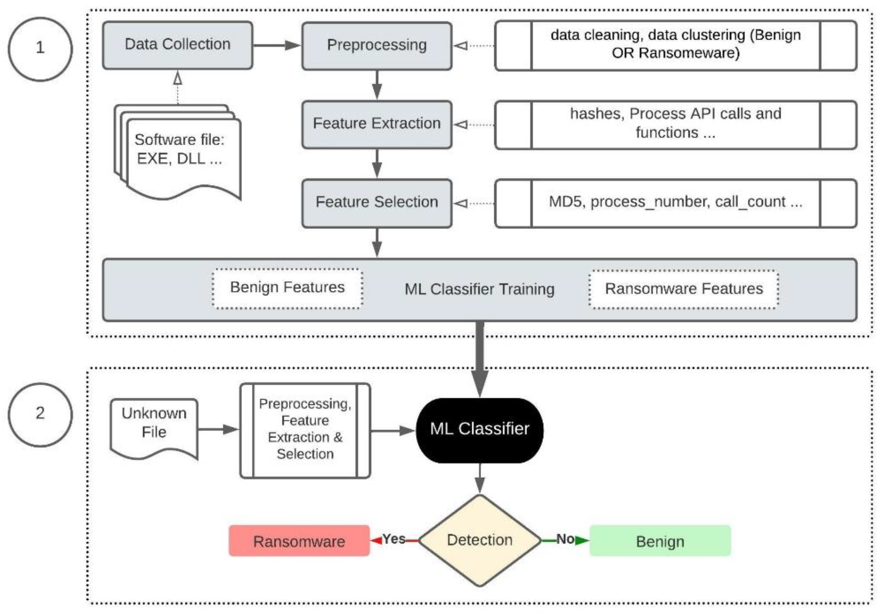
The methodology architecture is based on a ransomware detection model as illustrated in Figure 1. It consists of two steps, starting with the processes required to train a ML classifier and kept it up-to-date by utilizing more datasets as part of a data collection phase. The second step focuses on detection; the classifier is used to decide whether an unknown file is ransomware or benign. To reflect this in our experiment, we use virtual machines for malware analysis. The machines have been configured with a VirtualBox host-only network adapter to prevent malicious traffic from routing out of the sandbox environment. Two host machines were used for the experiments. The first, with an Ubuntu 20.04 operating system, was dedicated as a sandbox environment for executing malware and benign samples.

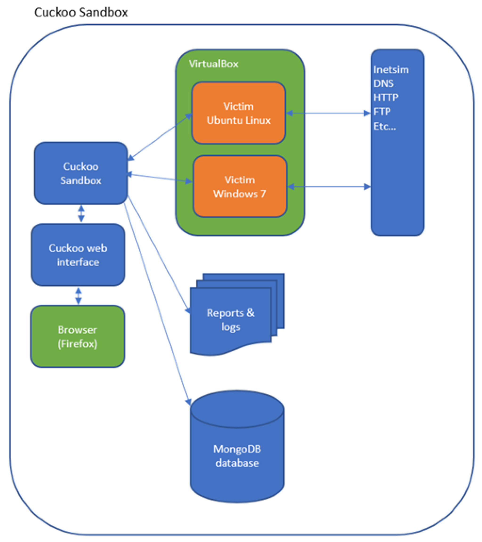
After the virtual machines were configured and the Cuckoo agent installed, snapshots were taken to restore the machines’ original configuration after each sample was analysed. INetSim was used to simulate the presence of internet services such as DNS and HTTP. Therefore, any requests made by malware under analysis would receive a fake response to DNS and HTTP requests. All DNS requests would resolve to the IP of the VirtualBox host-only network adapter. Other requests, such as HTTP, would receive a static file in response. The first environment is illustrated in Figure 2.

A second machine was solely built to train and deploy machine learning algorithms and to minimise any risk of malware ‘escaping’ the sandbox environment. The main software installed included Debian 10, Python 3, Scikit-learn [34], Tensorflow, MariaDB, and Microsoft Visual Studio Code.

3.2. Dataset Preparation

The ‘CryptoRansom’ archive [35] was the source of 38,157 samples, each named after its MD5 hash. Overall, 730 Malware samples were submitted to Cuckoo in batches using the web interface. To avoid class imbalance problems [26], 735 benign samples were also submitted. Benign samples were gathered from a Windows environment in the form of Executables and DLLs. The results from each sample were logged into a directory structure and a MongoDB database. The JSON files produced by Cuckoo were of particular interest due to the nature and quantity of information they contained. Each JSON file’s ‘apistats’ section had information about processes spawned by the sample, which process made API calls, and how many times each API function was called.

A bash script was used to rename all the report.json files to <task_id>.json, and copy them to a single directory. The files in this directory were then compiled into a compressed archive using tar and gzip. The resulting archive file was then transferred to the computer used for machine learning work, unzipped, and extracted.

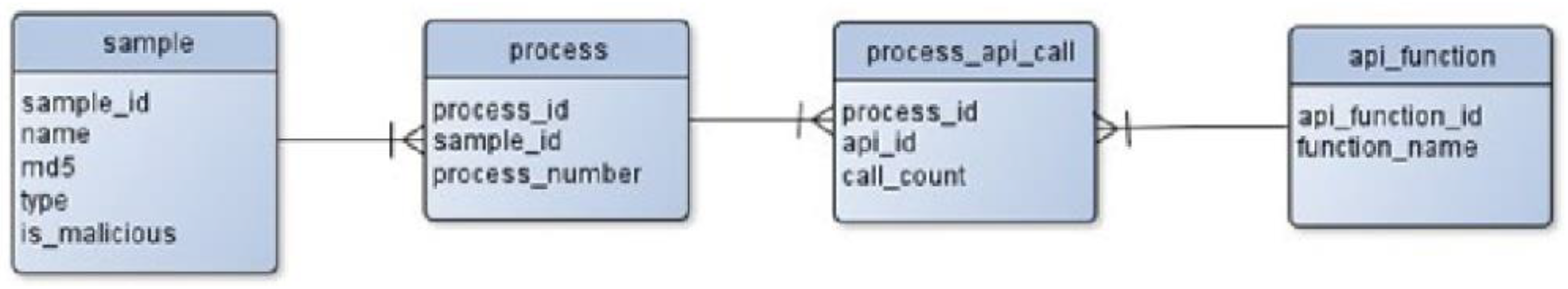
A MariaDB database was created to contain the statistics on API call frequency. The database schema is shown in Figure 3. This schema model shows that each sample spawned one or more processes, and each process made multiple API calls. Using a relational database allows the creation of different datasets using different queries. For example, it would be possible to produce a dataset containing information only on DLL samples or only for samples that spawn multiple processes. The database was populated from the collected JSON log files by a python script. Once populated, the record counts for each table were as shown in

Table 2. Database table record counts.

Table	Record Count
Sample	1465
Process	6341
process_api_call	269,918
api_function	284

.

A query to aggregate the API calls made by the processes spawned by each sample was run, and the results were output to a CSV file. A code example for the query is:

SELECT s.sample_id, s.is.malicious,

COUNT(p.process_id AS process_count, a.api_id,

SUM(a.call_count) AS call_count

FROM malware_stats.sample s

JOIN malware_stats.process p ON s.sample_id = p.sample_id

JOIN malware_stats.process_api_call a ON p.process_id = a.process_id

GROUP BY s.sample_id, s.is_malicious, a.api_id

The number of times malicious and benign samples called each API function was more than 565,902. Malicious samples called a wider range of API functions than benign samples, and overall malicious samples made more API calls than benign samples (8,607,508–929,971). The API functions most frequently called by malicious samples were: LdrGetProcedureAddress, ReadProcessMemory, NtClose, RegQueryValueExW, and NtReadFile; for benign samples, they were: NtReadFile, SetFilePointer, GetSystemMetrics, NtClose, and LdrGetProcedureAddress.

The API usage statistics were used to classify the examples as either benign or malicious. This data was re-arranged into a format suitable for training machine learning models by a script (csv_to_dataset.py) that uses pandas’ pivot table functionality. The resulting dataset contained 1465 labelled samples with the label ‘is_malicious’.

Each sample had 284 features, and each feature was the number of times the associated API function was called. The mentioned 284 features have integer values; therefore, no transformation of categorical features using one-hot encoding was necessary.

3.3. ML Algorithms

Machine learning algorithms suitable for binary classification problems [36] include Logistic Regression, Support Vector Machine, K-Nearest Neighbours, Decision Trees, Random Forests, and Artificial Neural Networks. Although linear regression is suitable for predicting a continuous quantitative value based on one or multiple features, it is not a practical approach for classifying samples as either benign or malicious. Still, it can stand as a valuable technique in understanding Logistic Regression. In contrast to linear, the logistic regression analysis method is specifically designed to predict a binary outcome. Based on an S-shaped curve generated by a sigmoid function (Formula (1)), a logistic regression model can determine the probability that the outcome lies in each of the two categories. β₀ is the bias that determines where the curve crosses the y-axis: positive values move the curve to the left, and negative values move it to the right. β₁ is the weight applied to feature x; this weight governs the rate at which p transitions from 0 to 1, with higher values giving a steeper gradient and sharper transition.

$$p=\frac{e^{{\beta }_0+{\beta }_{1^x}}}{1+e^{{\beta }_0+{\beta }_{1^x}}}$$

(1)

Formula (1): sigmoid function.

By adapting the linear regression approach, the formula can be extended for multiple features as follows (Formula (2)):

$$p=\frac{e^{{\beta }_0+{\beta }_{1^x}+{\beta }_2{x}_2+\dots {\beta }_n{x}_n}}{1+e^{{\beta }_0+{\beta }_{1^x}+{\beta }_2{x}_2+\dots {\beta }_n{x}_n}}$$

(2)

Formula (2): Logistic Regression sigmoid function.

Various statistical techniques can also be used to assess the goodness-of-fit of a logistic regression model, including the Pearson Chi-Square statistic and the Hosmer-Lemeshow test [37].

Support Vector Machines are considered particularly appropriate for datasets with a large number of features [38]. A dataset with two features could be visualised as a 2D graph in which the boundary is calculated to separate the two classes and maximise the margin between them. If more than two features are present, a hyperplane is calculated, similarly separating the two classes. Evaluation of examples against this hyperplane is then used to determine the classification.

The K-Nearest Neighbours can plot the values of training example features and attempt to classify new examples by determining the classification of the k-nearest examples seen in training [39]. The distance from the test example to its nearest neighbours is usually calculated as a Euclidean distance. If, for instance, the majority of the test example’s five nearest neighbours are positive, the test example’s classification would also be positive.

Decision trees have long been used as a manual aid to decision-making, for instance, in clinical diagnosis [40]. Like flowcharts, a decision tree consists mainly of decision nodes (leaves), each with two possible outputs—malicious or not.

While decision trees are easy to comprehend, they have some disadvantages. They can be prone to over-fitting-reflecting the particular characteristics of training data too closely and therefore becoming less effective for making predictions [41]. Anomalous outliers can also unduly influence them in training data [42].

To overcome the disadvantages of Decision Trees, Breiman [43] developed Random Forests. A Random Forest consists of a number of decision trees, each trained on either a subset of training examples (bagging) or a subset of features. A voting mechanism is then used to determine the final classification based on the results of multiple trees. Breiman uses the Strong Law of Large Numbers to show that Random Forests are not susceptible to overfitting and are not unduly influenced by outliers in the training data.

Artificial Neural Networks consist of a series of layers—an input layer, a hidden layer, and an output layer. Each layer consists of several nodes that take a number of inputs, perform a calculation, and produce one output. Layers are typically connected densely such that the outputs of each node in the input layer act as inputs to nodes in the hidden layer. Similarly, the outputs of hidden layer nodes act as input to nodes in the output layer. Each connection between nodes in different layers is assigned a weight which is optimised during the training process. Each node has an activation function that determines whether the node is active or not based on its inputs. The nodes in a given layer all have the same activation function. Common activation functions are Rectified Linear Unit (ReLU), the sigmoid function previously described, and the hyperbolic tangent function.

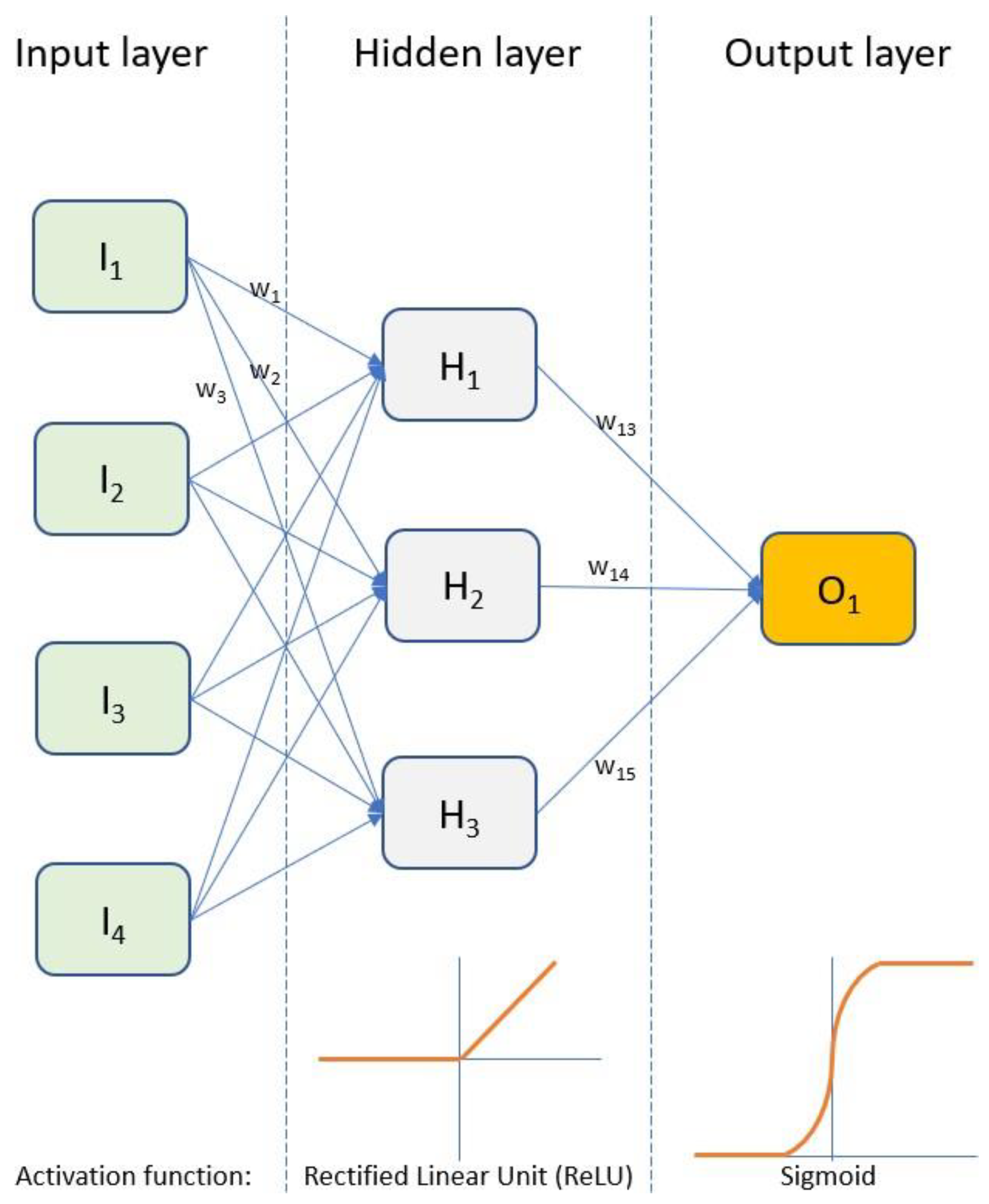
The number of layers (there can be more than one hidden layer), the number of nodes in each layer, and the activation functions used will be influenced by the problem the network is designed to solve and the expertise of the network designer. In addition to the parameters mentioned above (number of layers, nodes per layer, activation functions), other hyper-parameters, such as the number of training epochs and the evaluation batch size, must be considered. A simple neural network for binary classification is shown in Figure 4.

This network takes four inputs I₁ to I₄. The input values are weighted according to the weights w₁, w₂…w₁₂ and passed to nodes in the hidden layer. Each node in the hidden layer uses the ReLU function to determine its output. The ReLU function returns 0 if the input is negative or returns the input value. These outputs are again weighted (w₁₃, w₁₄, and w₁₅) and passed to a single output node. The output node uses a sigmoid function to determine whether the final classification should be 0 or 1.

The network is trained on a set of training data through multiple epochs. After each epoch, the network’s effectiveness is evaluated using a loss function. Adjustments are made to the weight values before the next epoch starts. Evaluation is typically not performed for the whole training dataset; instead, a small batch of samples is used. Over multiple epochs, the values for weights w₁ to w₁₄ are refined.

4. Evaluation

4.1. Evaluation Metrics

For all the mentioned algorithms, a binary classifier will produce a confusion matrix that depicts the number of correctly and incorrectly classified positive and negative samples—True Positives (TP), True Negatives (TN), False Positives (FP) and False Negatives (FN). In this section, the metrics widely used in evaluating the performance of machine learning models will be presented, all calculated from the four values in the confusion matrix.

The first metric is Accuracy (A). This metric evaluated the models’ classification, as it is the fraction of predictions that the model predicted correctly. It is calculated by dividing the number of correct predictions by the total number of predictions, expressed as a percentage (Equation (3a)). When considered in isolation, Accuracy can be misleading if classes are not represented equally in the dataset, i.e., in case of a class imbalance. For a dataset containing 95% malicious samples and 5% non-malicious, a model that predicted ‘malicious’ 100% of the time would achieve 95% accuracy.

The Precision (P) ratio quantifies the true positives in relation to the total of true positives and false positives (Equation (3b)) and describes the proportion of correct positive classifications. Where a class imbalance exists, the precision can be calculated for each class to indicate whether the imbalance affects the model’s ability to classify correctly. Since a false negative result is a misclassified positive, this metric expresses the proportion of the examples classified as positive as a proportion of the overall number of actual positives.

The True Positive Rate (Equation (3c)) is also referred to as Recall and Sensitivity. Since a false negative result is a misclassified positive, this metric expresses the proportion of examples that were classified as positive as a proportion of the overall number of actual positives.

The False Positive Rate (FPR) is the proportion of all negatives that still yield positive test outcomes, or the misclassified negatives. The FPR is the number of false positives (i.e., misclassified negatives) divided by the total number of negatives (Equation (3e)). This is the likelihood that a positive will be predicted for an actually negative example.

The True Negative Rate (TNR) is also referred to as specificity. As already noted, false positives are misclassified negatives. The true negative rate is the number of true negatives divided by the total number of actual negative values (Equation (3f)). It measures how accurate the model is at making negative predictions.

The opposite of the TNR, the False Negative Rate (FNR), represents misclassified positives. It measures the number of misclassified positives as a proportion of the total number of positives (Equation (3g)). The F1 score, a machine learning metric, was also used in the classification process of the models by calculating the weighted average of Precision and Recall. Recall describes the proportion of true positive predictions to actual positives, and precision represents the proportion of true positive predictions to the total of true positives and false positives (Equation (3d)). The F1 score combines these two values, producing a harmonic mean of TPR and precision. The F1 score takes a value between 0 and 1, and a value of 1, indicating no false positives and no false negatives, is optimal.

$$Accuracy A=\frac{TP+TN}{TP+FP+TN+FN}$$

(3a)

$$Precision P =\frac{TP}{TP+FP}$$

(3b)

$$True Positive Rate P =\frac{TP}{TP+FN}$$

(3c)

$$F\mathit{1} Score f =\frac{2TP}{2TP+FP+FN}$$

(3d)

$$False Positive Rate FPR=\frac{FP}{FP+TN}$$

(3e)

$$True Negative Rate\left(Specificity\right) TNR=\frac{TN}{TN+FP}$$

(3f)

$$False Negative Rate FNR=\frac{FN}{FN+TP}$$

(3g)

Equations (3a–g): Evaluation Metrics, (a) Accuracy, (b) Precision, (c) True Positive Rate, (d) F1 Score, (e) False Positive Rate, (f) True Negative Rate, (g) False Negative Rate.

4.2. Metrics

The following metrics were calculated according to the Equation set out by Kok et al. (2020).

The Likelihood Ratio (LR) was used to indicate how well the model distinguishes between benign and malicious samples. Two Equations were given for LR—Positive Likelihood Ratio (PLR) (Equation (4a)) and Negative Likelihood Ration (NLR) (Equation (4b)). PLR indicates how well the model distinguishes benign samples from malicious ones. A value of 10 or more shows that the model distinguishes well. An NLR of less than 0.1 also indicates that the model distinguishes well between benign and malicious samples.

The Diagnostic Odds Ratio (Equation (4c)) was also used to calculate the ratio of PLR to NLR, in which the higher values are better.

The Youden’s Index measures incorrect predictions. A model producing no False Positives and no False Negatives would have a Youden’s index of 1 ((Equation (4d)).

According [17] the Number Needed to Diagnose (NND) (Equation (4e)) metric describes the number of samples needed for the model to make a correct positive prediction.

The Number Needed to Misdiagnose (NNM) metric is the number of samples needed for the model to make one incorrect prediction. In this formula, n is the total number of samples (Equation (4f)).

The Net Benefit (NB) determines whether the predictive model has provided a correct or incorrect prediction based on a cutoff point in terms of a probability threshold (P) (Equation (4g)). The idea is taken from the medical field [44]. NB is used to balance the value of an investigation, such as a biopsy, against the potential for harm, such as conducting unnecessary biopsies for a given indication that a condition may exist. Unnecessary biopsies have associated risks such as infection, patient pain, and the use of resources. NB is used in the medical field to apply weight, which Vickers et al. refer to as an ‘exchange rate’, to the disadvantages of investigating false positives compared to the harm of missing a positive diagnosis. It should also be noted that in Vickers et al., N refers to the total sum of true and false-positive results—negative results are not in scope. Vickers et al.’s original formula was used when calculating NB.

Receiver Operator Curves (ROC) are a way of graphically depicting the effectiveness of a binary classification model. They are frequently used to assess the diagnostic value of clinical tests [45]. In a ROC, the True Positive Rate (sensitivity) is plotted on the y-axis against the False Positive Rate on the x-axis. The x-axis is usually titled “1—specificity” in clinical contexts, where specificity is the True Negative Rate. The value of (1—specificity) is the same as the False Positive Rate. The x-axis is usually labelled “False Positive Rate” in machine learning contexts. An ideal classifier would have an AUC of 1, and a classifier with no ability to discriminate would have an AUC of 0.5.

$$False Negative Rate FNR=\frac{FN}{FN+TP}$$

(4a)

$$Negative Likelihood Ratio NLR=\frac{TPR-1}{TNR}$$

(4b)

$$Diagnostic Odds Ratio DOR=\frac{PLR}{NLR}$$

(4c)

$$Youden’s index J = TPR+TNR-1$$

(4d)

$$Number Needed to Diagnose NND =\frac{1}{\left[TPR-\left(1-TNR\right)\right]\frac{1}{J}}$$

(4e)

$$NM=\frac{1}{\left[1-\frac{\left(TP+TN\right)}{n}\right]}$$

(4f)

$$Net Benefit NB=\left(\frac{TP}{n}-\frac{FP}{n}\right)\frac{P}{1-P}$$

(4g)

Equations (4a–g): Novel metrics, (a) Positive Likelihood Ratio, (b) Negative Likelihood Ratio, (c) Diagnostic Odds Ratio, (d) Youden’s Index, (e) Number Needed to Diagnose, (f) Number Needed to Misdiagnose, (g) Net Benefit.

5. Experiment Description

A logistic regression model was built in Python using Scikit-learn [34]. The dataset file was prepared as follows. The sample_id column was removed to prevent it from influencing the model. Malicious samples were analysed first during sample analysis, followed by benign samples. The sample_id was taken from the Task ID generated by the Cuckoo Sandbox software and used as the primary key in the samples database table. Consequently, all malicious samples had a sample_id of 830 or less, and all benign samples had a sample_id of greater than 830. The sample_id column would have undoubtedly influenced the model, invalidating it if not removed. Labels were extracted from the is_malicious column into a separate array and dropped from the dataset. The complete dataset was split into training and testing sets with a ratio of 80:20, using Scikit-learn’s train_test_split functionality. Training data features were scaled using a StandardScaler, which centers the data around its mean and scales by its standard deviation. Each feature value is scaled according to the formula (Formula (5)).

$$Z=\frac{\left(x-u\right)}{\sigma }$$

(5)

Formula (5): StandardScaler formula.

Where x is the observed value of a feature, u is the mean value of the feature across all examples, and σ is the standard deviation of the feature values. The logistic regression model was trained on the scaled data and tested using a version of the test data that had been scaled using the same StandardScaler instance used to mount the training data, described in Section 3.

For Support Vector Machine the dataset was prepared and split similarly to the logistic regression model, and a series of SVM models were built using Scikit-learn’s SVC classifier. Four models were created using the Radial Basis Function (RBF), Linear, Polynomial, and Sigmoid kernel functions.

After the preparation and splitting of the dataset, a K-Nearest Neighbours model was built using Scikit-learn’s KNeighborsClassifier. The algorithm selection was left at the default of ‘auto’, which selects a brute-force algorithm for determining the distances between neighbours. The k-value was set to the default value of 5.

For the Decision Tree model, similarly to the logistic regression model, the dataset was loaded from a CSV file and prepared by removing the sample_id column, extracting labels, and scaling features using a StandardScaler. The dataset was then split into a training set (80%) and a testing set (20%).

The model was built using Scikit-learn’s DecisionTreeClassifier and trained using the training data. The model’s performance was evaluated against both the training and testing data. Suspicions of overfitting were investigated, and a revised model was subsequently built.

The dataset was loaded and prepared similarly to the logistic regression and decision tree models for the Random Forest model. A random forest model was built using the Scikit-learn RandomForestClassifier, trained, and had its performance evaluated against training and testing data.

The dataset was prepared, scaled, and split for the Artificial Neural Network model as before. Tensorflow was used to create a neural network which could then be trained and evaluated. The network’s configuration was as follows: input layer—284 units (to match the number of input features); activation function—Rectified Linear Unit; hidden layer—experiments were conducted with a hidden layer of 16 units (NN-16), 64 units (NN-64), and 128 units (NN-128); output layer—1 unit with activation function: sigmoid. The activation function was Rectified Linear Unit in each case.

The model was trained for 100 epochs, and metrics were calculated. Regarding the metrics such as accuracy, precision, and the area under the ROC curve, there was little difference between the NN-16 and NN-64 networks, and the metrics were slightly worse for NN-128. Further developments of the neural network model continued to use 16 units in the hidden layer.

6. Results

The metrics calculated fell into two categories: commonly used, and those proposed by Kok et al. [17]. The metrics are described in Section 4, and their values are summarised in

Table 3. Comparison of metrics for different models.

Metric	SVM	KNN	Logistic Regression	Decision Tree	Random Forest	Neural Net ANN Model (3)
True Positive	144	147	143	152	153	146
True Negative	138	133	137	134	128	138
False Positive	2	7	3	6	12	2
False Negative	9	6	10	1	0	7
Accuracy	96.25%	95.56%	95.56%	97.61%	95.90%	96.93%
True Positive Rate	94.12%	96.08%	93.46%	99.35%	100.00%	95.42%
False Positive Rate	1.43%	5.00%	2.14%	4.29%	8.57%	1.43%
True Negative Rate	98.57%	95.00%	97.86%	95.71%	91.43%	98.57%
False Negative Rate	5.88%	3.92%	6.54%	0.65%	0.00%	4.58%
Precision	98.63%	95.45%	97.95%	96.20%	92.73%	98.65%
F1-Score	96.32%	93.11%	95.65%	97.75%	96.23%	97.01%
Area under ROC curve	97.62%	98.97%	97.32%	97.70%	99.84%	97.54%
Positive Likelihood Ratio (1)	65.88	12.99	43.62	15.45	11.67	66.8
Negative Likelihood Ratio (2)	−0.06	−0.08	−0.07	−0.01	0	−0.05
Diagnostic Odds Ratio (3)	−1104	−167.82	−653.03	−2212.44	<div by zero>	−1439.14
Youden’s Index	0.93	0.86	0.91	0.93	0.91	0.94
No. Needed to Diagnose (4)	1	1	1	1	1	1
No. Needed to Misdiagnose	26.64	13.92	22.54	29.3	24.42	32.56
Net Benefit (p = 0.10)	76.25%	−18.47%	64.38%	29.10%	−41.48%	76.27%

.

The PLR values were above ten, indicating a good ability to classify benign samples from malicious ones. Similarly, the NLR values were below 0.1, providing the same classification levels. With regard to the DOR and according to KoK et al. [17], these values can range from 0 to infinity, with values above 100 indicating a good predictive power of the model. Since we have negative NLRs, these values are actually less than zero. The NND values, as was already described in Section 4, constantly evaluate to 1. Finally, the Net Benefit has been calculated at p = 0.10, analogous to investigating nine false positives for every true positive detected.

The tendency of decision trees to overfit their training data, and be influenced by anomalous training data, has previously been documented (Dietterich, 1995) [41]. The original decision tree model exhibited overfitting. The revised decision tree model, limited to a maximum depth of eight levels, produces fewer false positives, more true negatives, and higher accuracy, precision, and area values under the ROC curve.

Overfitting is also a common problem with neural networks. ANN Models 1 and 2 exhibited severe overfitting. A model suffering from overfitting has been unduly influenced by noise in the training data. It is easier to make predictions based on the training data, but the results are increasingly poor when making predictions on unseen data (the testing data).

Overfitting was resolved in ANN Model 3 by using tanh as the activation function in the hidden layer and adjusting the number of training epochs. 50 Epochs were found to be optimum by repeated experimentation. The testing and training loss curves were closely aligned, which is evidence that the model is not overfitted. Other potential strategies for reducing overfitting include increasing the evaluation batch size and the number of hidden layers in the network.

6.1. Importance of False Negatives

Petticrew et al. [46] describe the potential disadvantages resulting from false negatives generated by healthcare screening programmes. False negatives can result in cases of the disease being missed and delayed treatment. Missed cases and delayed treatment can lead to psychological harm for the affected patients and the possibility of legal action, with its associated financial impact on the screening organisation. In severe cases, the credibility of a screening programme might be undermined by false negatives, leading to reduced participation in the programme, which could drastically reduce the benefits of conducting the screening programme in the first place.

Similarly, a false negative could be the worst prediction a ransomware detection model could make. While this has been recognised in clinical fields as described above, the importance of false negatives in ransomware and malware detection does not appear to have received the same attention. Accuracy is often given undue weight when determining the performance of models in previous papers, which, as previously stated, does not necessarily provide an accurate picture of the model’s performance. In previous articles, there is also less consideration of the False Negative Rate compared to the True Positive and False Positive Rate. In a practical application, such as the classification of ransomware, the False Negative rate should be given more consideration since the consequences of a false negative are potentially very damaging.

6.2. Comparison of Metrics

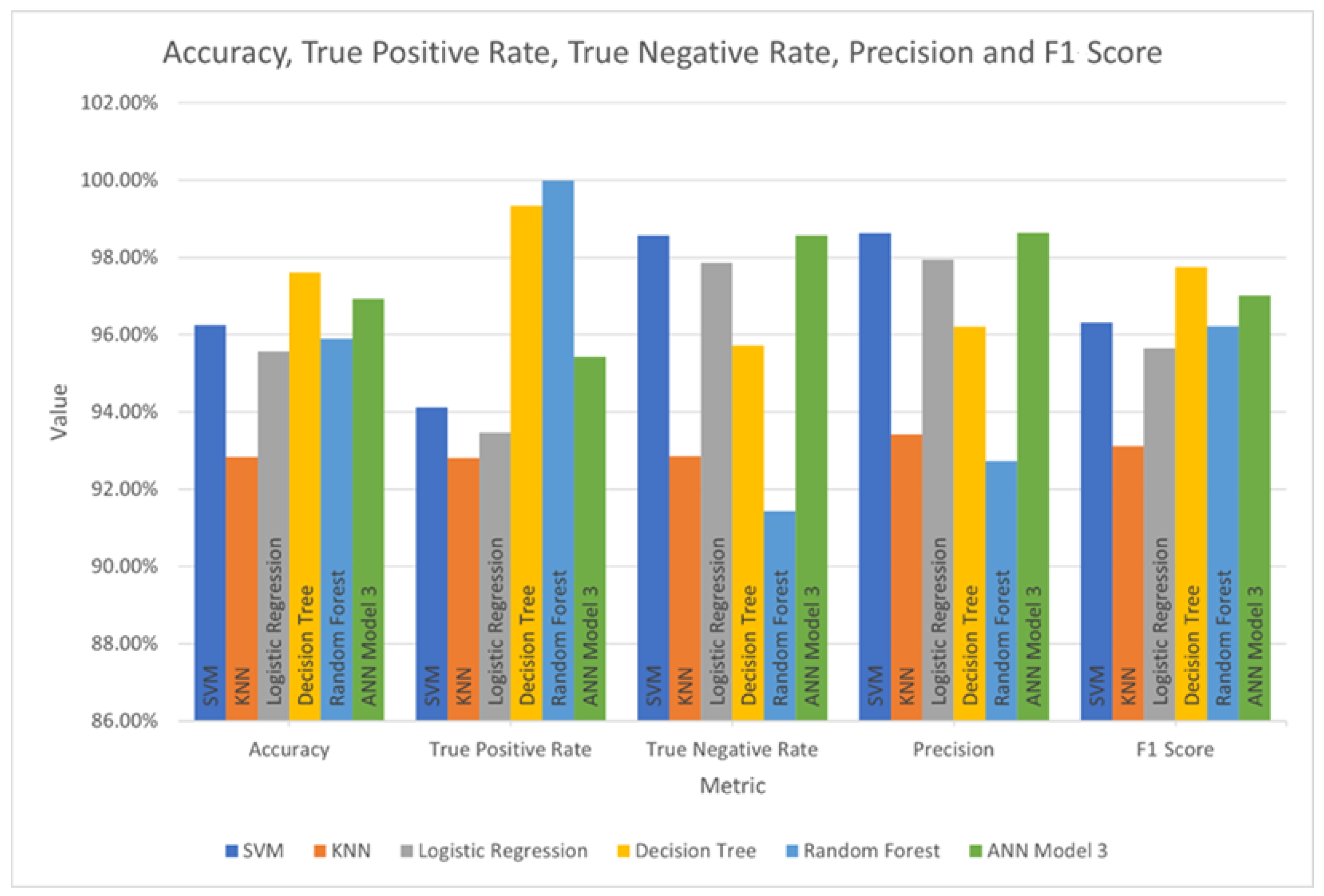
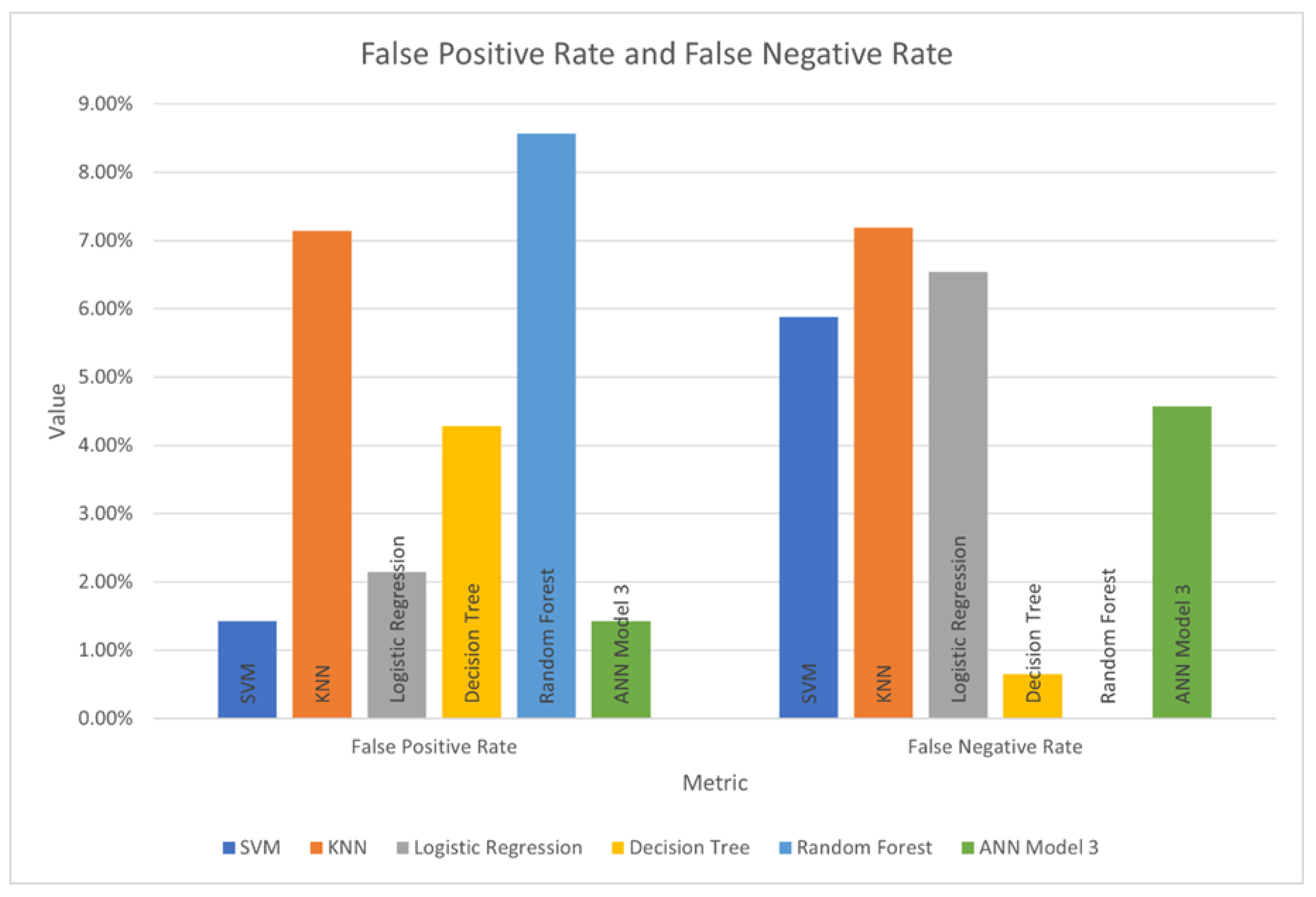
To facilitate comparison between the models, the metrics for each model are charted in Figure 5, and false positive and false negative rates are charted in Figure 6.

The KNN model does not achieve high values for accuracy, true positive rate, true negative rate, precision, or F1 score. While the values of these metrics for the SVM model are higher, both the SVM and KNN models have a high false-negative rate, making them unsuitable for the classification of ransomware.

The Logistic Regression model scores slightly lower than the SVM model for accuracy, TPR, TNR, precision, and F1 score. However, the false-negative rate for logistic regression is higher than that of the SVM model. Because of these factors, it is a worse classifier choice than SVM.

The Decision Tree model achieves the highest accuracy and F1 score, with a false-negative rate of only 0.65%. This would make it a good choice as a classifier, but the tendency of decision trees to overfit to training data must be weighed against this.

Random Forest achieves the best true positive rate, but the values for accuracy, true negative rate, precision, and F1 score are unexceptional. However, it should be noted that the Random Forest model produced a false negative rate of 0.00%.

ANN Model 3 achieved good values for accuracy, true negative rate, precision, and F1 score. It is in the top two scores across most of the metrics shown in Figure 5. While this indicates successful classification, the false-negative rate of 4.58% is a concern.

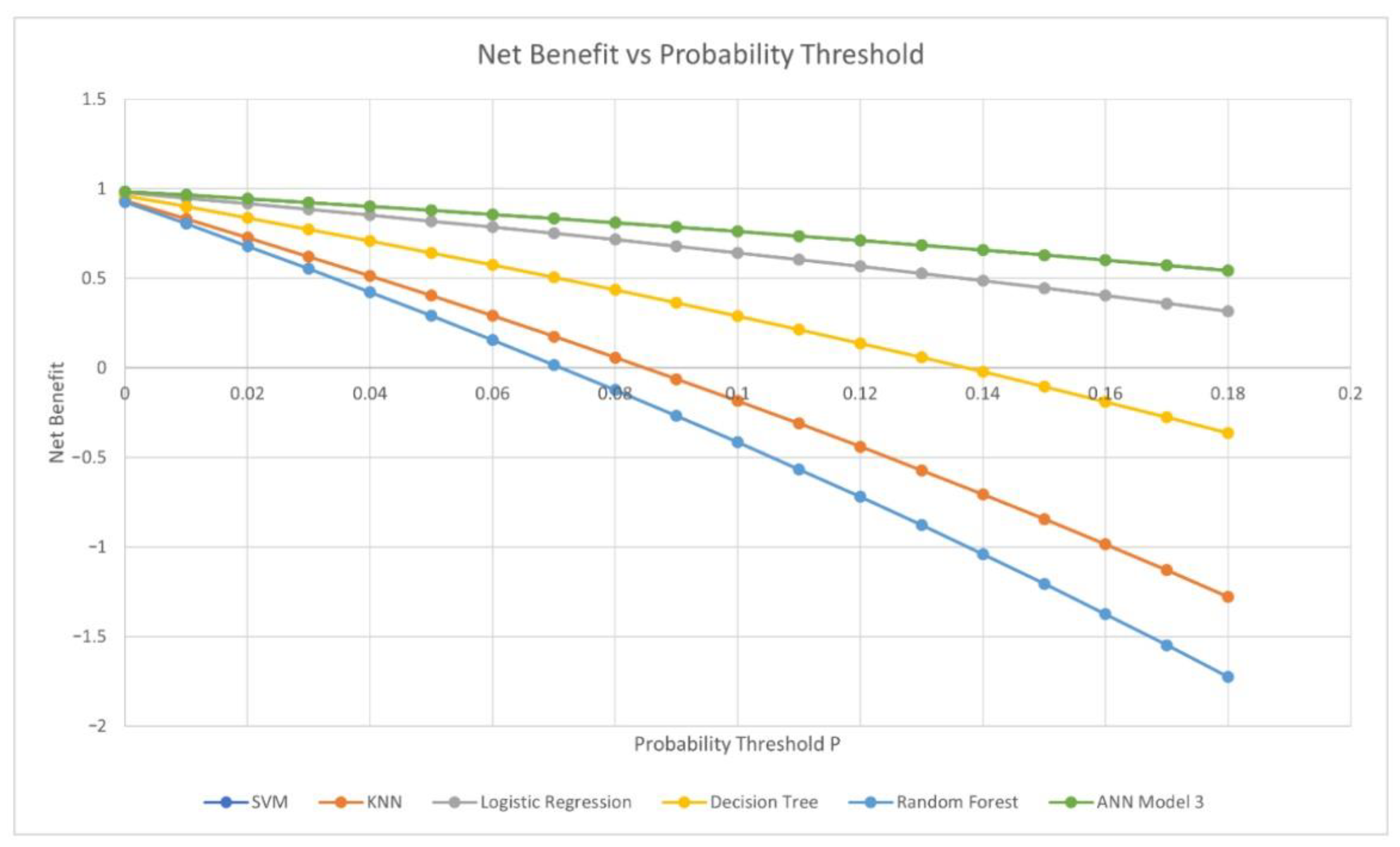
The Net Benefit for a range of probability thresholds, calculated according to Vickers et al.’s formula [44], is plotted for each model in Figure 7. All have a positive Net Benefit for values of p ≤ 0.07, with ANN Model 3 and the logistic regression model providing the greatest Net Benefit.

If the models were to be judged on accuracy alone, it would appear that the Decision Tree and ANN Model 3 are the most capable, with accuracies of 97.61% and 96.93%, respectively. The F1-score is a more useful metric since it is based on recall and precision values. The F1-scores for these two models are also good, at 97.75% and 97.01%, respectively. If Net Benefit were to be used as the sole criterion, it would appear that ANN Model 3 and the logistic regression model would give the best classification performance. However, the consideration of other metrics reveals more about the characteristics of each model, which could influence their suitability for detecting ransomware.

The worst prediction a ransomware detection system could make would be a false negative, i.e., to incorrectly classify ransomware as non-malicious. The comparatively high false-negative rates for the logistic regression (6.54%) and the ANN Model 3 neural network (4.58%) models suggest that these models should be used cautiously to detect ransomware (Figure 6).

Due to the critical nature of the task of identifying ransomware, and the negative consequences of a false negative classification, a more ‘cautious’ model may be preferred. While the random forest model does not have the highest accuracy or precision, the model’s True Positive Rate of 100% and False Negative Rate of 0% suggest that its classifications are more ‘cautious’ than classifications produced by the other models. It has a tendency to classify benign samples as ransomware and appears unlikely to classify ransomware as benign. For this reason, the random forest model might be considered the ‘safest’ of the models evaluated for the task of ransomware identification.

This illustrates the risks of relying solely on metrics to judge the suitability of a model without considering the nature of the classification problem, the risk appetite of those interpreting the prediction, and the consequences of false negatives in particular. Although by most metrics (accuracy, precision, F1-score, and Net Benefit), ANN Model 3 produces the best performance, its false-negative rate of 4.58% means its predictions should be treated with caution.

7. Discussion

Comparisons with the results of previous work are not straightforward because the full range of metrics is often not quoted. Specifically, the raw values of True Positives, True Negatives, False Positives, and False Negatives are often omitted. As discussed earlier, these four values are the basis of all the other metrics discussed. The quoted results from relevant publications are summarised in

Table 4. Comparison with results from previous work.

Paper	TPR	FPR	TNR	FNR	Accuracy	Precision	Recall	F1 Score
(RF)	100.00%	8.57%	91.43%	0.00%	95.90%	92.73%	100.00%	96.23%
(ANN Model 3)	95.42%	1.43%	98.57%	4.58%	96.93%	98.65%	95.42%	97.01%
[25]	n/a	1.60%	n/a	n/a	n/a	98.60%	99.40%	98.60%
[32]	n/a	n/a	n/a	n/a	97.30%	n/a	n/a	n/a
[33]	n/a	n/a	n/a	n/a	98.65%	98.25%	98.94%	98.54%
[26]	98.45%	1.50%	n/a	n/a	n/a	98.50%	98.50%	98.50%
[28] SVM	n/a	n/a	n/a	n/a	98.80%	98.50%	100.00%	99.30%
[28] MLP	n/a	n/a	n/a	n/a	100.00%	100.00%	100.00%	100.00%

.

Where values were not given, the table cells have been shaded grey and labelled ‘n/a’. The results quoted by Ahmed et al. (2020) relate to their SVM model with a feature set size of 90 features, each feature being an n-gram of system calls with n = 3. The EmRmR algorithm was used to remove ‘noise’ API calls from ransomware traces. The values for Accuracy, Recall, and Precision were all good, but no figures were given for True Positive Rate, True Negative Rate, or False Negative Rate. Emphasis was placed on the False Positive Rate of 1.60%, which is arguably not the most important metric for a ransomware detection system.

Asmitha et al. [32] achieved the statistics quoted above using Odds Ratio to achieve feature reduction and a Random Forest algorithm. The effectiveness of the models tested is assessed purely based on accuracy.

Bae et al. [33] implemented a three-way algorithm which classified samples into Benign, Malware, and Ransomware categories. They proposed a Class Frequency—Non Class Frequency (CF-NCF) algorithm to generate n-grams. They achieved an accuracy of 99.05% using a random forest algorithm with n = 3 when distinguishing between ransomware and benign samples. However, in their comparison with other classification methods, they quote an accuracy figure of 98.65% (Table 4), which is achieved by the random forest algorithm with 1-g. The discussion of the results is again framed in terms of accuracy, so the tendency of their models towards false positives or false negatives is not discussed.

Sheen et al. [26] quote slightly different figures for TPR and Recall. These are different names for the same metric, so the reason for this is not clear. They note that their dataset was imbalanced between ransomware and benign classes. They describe their use of SMOTE to address this imbalance and demonstrate improvements in the accuracy of their models after the application of SMOTE. Again, there is an emphasis on the true positive rate and false-positive rate, with the true and false-negative rates not discussed.

The Support Vector Machine and Multi-Layer Perceptron results from Vinayakumar et al. [28] are very encouraging, but their detailed analysis of their performance against different ransomware families shows that these algorithms were less capable of identifying CryptoLocker and CryptoWall ransomware. The detailed analysis shows accuracies of 97.6% for SVM and 98.0% for MLP. This is in contrast to the headline metrics for the MLP model, where Accuracy, Precision, Recall, and F Score all reach 100%.

8. Future Work

It would be beneficial to expand the API statistics database by analysing more malicious and benign samples. A broader source of benign samples from vendors other than Microsoft would reflect different coding styles and may increase the number of false positives observed.

The samples analysed for this study gave rise to a dataset with 284 features. As more samples are analysed, the number of features will likely increase, as well as the number of examples. The time and computing power required to train models on the resulting larger, more feature-rich datasets will also increase. The use of feature reduction and feature engineering could be investigated to reduce the number of features and therefore reduce the time and computing power required to train models.

The attempts to resolve the overfitting exhibited by ANN Model 1 and ANN Model 2 were successful, with the training and testing loss curves tracking closely over 50 epochs. The performance of ANN Model 3, when judged by most metrics, was superior to that of the other models, let down only by its false-negative rate. Further development of ANN Model 3 could include novel means aiming to reduce its false negative rate, which at 4.58% is still a cause for concern, without impacting its accuracy, precision, F1 score, or Net Benefit.

In addition to the web interface, Cuckoo also provides a REST API interface. This interface could be leveraged so that samples can be submitted remotely by a REST client. Once the sample analysis is complete, the client would then retrieve the appropriate log file, parse out the API usage statistics, update the database seamlessly, make a prediction using the trained model, and report the prediction back to the user. Creating such an integrated system would allow samples to be analysed relatively quickly by users who do not have the technical knowledge required to run scripts, perform file transfers, execute SQL queries, and prepare datasets. Additionally, future work could include the development and release of a prototype open-source tool that integrates the contextual and novel evaluation metrics to test and compare the performance of ML algorithms for ransomware detection.

9. Conclusions

This paper examined and tested the suitability of six machine-learning algorithms for ransomware detection. The experiments performed in this study utilised Windows API call frequency analysis as an approach for identifying ransomware efficiently. The produced samples were balanced to avoid under-sampling/over-sampling [26]. However, it is essential to acknowledge that the number of positive samples (malware) under contextual circumstances could significantly vary between applications in real-world scenarios (e.g., would be less in normal circumstances), which poses a limitation and a challenge for this type of research.

In response to our research questions ((1) which error parameters and evaluation matrices should be utilised by the state-of-the-art to discuss the reliability of ML models for the detection of ransomware, and (2) which ML models offer reliability for the detection of ransomware?), we have utilized and tested several metrics, such as the Positive Likelihood Ratio, Negative Likelihood Ratio, and Diagnostic Odds Ratio. However, the study emphasized the importance of false negatives in preventing a potentially large cost of a ransomware infection.

Overall, we trained and evaluated three Artificial Neural Network (ANN) models based on six algorithms: Support Vector Machine, K-Nearest Neighbours, Logistic Regression, Decision Tree, Random Forest, and Artificial Neural Network. After the models were trained and evaluated, metrics were calculated to allow a comparison to be made. The ANN model 1, with a hidden layer of 16 nodes using ReLU activation function and trained for 100 epochs, was the most time-consuming to train. The decision tree and early iterations of the neural network models ANN Model 1 and ANN Model 2 (trained for 40 epochs) suffered from overfitting. After considerable experimentation, overfitting of the ANN models was overcome in ANN Model 3 by using the tanh function and by adjusting the number of epochs over which the model was trained. Although the Random Forest algorithm did not achieve the highest accuracy and reached the lowest precision metric, as it was more likely to classify non-malicious examples as malicious and less likely to classify malicious examples as non-malicious, it might be considered the safest of the six algorithms for ransomware identification. Finally, the ANN Model 3 achieved the highest from the models’ true-negative rate and precision values. If the false-negative rate could be reduced with further tuning and/or training on a larger dataset, ANN Model 3 would be the optimum choice for ransomware classification. A more comprehensive source of benign samples from vendors other than Microsoft would also reflect different coding styles and may increase the number of false positives observed.