Assessment of Adjustment of GNSS Railway Measurements with Parameter-Binding Conditions in a Stationary Scenario

Abstract

The study aims to assess the applicability of the ordinary least squares method, robust estimation, and conditions-binded adjustment in processing the six synchronous coordinate pairs of global navigation satellite system (GNSS) receivers. The research is part of the research project InnoSatTrack, focused on the enhancement of the determination of geometrical parameters of railway tracks using GNSS, inertial, and other sensors. A fixed frame of installation of six receivers is used in the data processing. Due to the limited availability of railway routes for measurements, the stationary campaign was conducted to gather data for the adjustment procedures tests. Six GNSS receivers in the frame-restricted configuration were set up using the tachymetric method for recording 96,729 synchronous static observations. Post-processed coordinates of the receivers were adjusted according to the geometrical conditions of the survey frame. Analysis showed higher applicability of the conditions-binded method than other estimation methods by obtaining superior results in both the precision and the maintenance of the design conditions factors than in the OLS and robust estimators.

1. Introduction

Determination of the geometrical parameters of a railway track is an important design factor preceding both the construction of a railway line [1] and its maintenance [2]. Assessing the degradation of the railway track quality involves, e.g., the determination of the degree of wear of the rails and the changes in the railway track geometry [3,4]. It should be noted that the quality of the track also affects the interaction performance between the train and the overhead infrastructure [5,6]. Control surveys employ various survey technologies using, e.g., mobile laser scanning [7], axle box acceleration devices [8], trolley system and total station [9], global navigation satellite system (GNSS) observations [10,11], inertial measurement units [12], and vision systems [13]. The literature also describes advanced methods for connecting multiple sensors on a single survey platform [14,15,16].

The processing of datasets obtained from multiple sensors involves the introduction of advanced computational methods focused on, e.g., point clouds registration [17], determining the positions of navigation satellites connected with post-processing of satellite data [18], and the joint calculation of both GNSS and inertial data [19]. The crucial point in the data processing is the synchronization of time-tagged observations obtained in different time systems, e.g., GPS time, BeiDou time, and coordinated universal time (UTC) [20]. An additional aspect is the adoption of uniform implementation of the International terrestrial reference system (ITRS) or European terrestrial reference system (ETRS) system [21] and if it is needed, appropriate map projection functions [22].

The development of the GNSS resulted in a significant increase in the number of available satellites [23]. Satellites of the GPS, GLONASS, Galileo, and BeiDou systems circulate on the medium Earth orbits (MEO). Additionally, the BeiDou system uses the geostationary (GEO) and inclined geosynchronous (IGSO) satellites [24] that enhance the positioning services in the Far East region. The increasing availability of navigation satellite signals was a motivation for studies that used several GNSS receivers in measurements of railway and tramway routes [25,26,27]. An important milestone was the InnoSatTrack project, which addressed the issues of efficiency, accuracy, and applicability of satellite positioning techniques in Polish national railways.

In the InnoSatTrack project, a low-sideboard railway carriage designed for transporting coal and iron ore was adopted as a mobile railway platform for advanced railway surveys [28]. A multi-modal system of frames and custom supports was constructed to enable the installation of various devices, e.g., GNSS receivers, accelerometers, vision systems, mobile laser scanners, and inclinometers [29]. The introduction of active geodetic networks [30] services was also used to assess the accuracy parameters of several mobile devices used in sports and recreational applications [31]. The project aimed to increase the accuracy and efficiency of determining the geometric parameters of railway tracks compared to previously used measurement methods.

A uniform structural frame for sensor support was used in several measurement campaigns during the project. The core devices were GNSS receivers that followed the railway track axis due to the installation above two platform kingpins. The remaining four receivers were installed on the sides of the platform above the railway tracks. The tachymetric method was used to ensure the millimeter accuracy of the installation of devices with fixed linear and angular conditions. In the tachymetric measurement, the three-dimensional coordinates of a point are calculated based on slope distance and horizontal and vertical angles. This solution enables the application of various adjustment methods, e.g., conditions-binded adjustment [32], the standard ordinary least squares (OLS) method, robust estimation with dumping functions [33,34,35,36], or the M-estimation [37,38].

Estimates of coordinates that maintain the design geometry between six GNSS receivers are used in joint processing resulting in the determination of the railway axis and other track parameters. However, the synchronous six-receiver dynamic registration along the railway route is frequently limited by the lack of redundant observations. The conditions and regulations for rail traffic also limit the possibility of the temporary exclusion of selected routes from standard use to conduct survey campaigns using the mobile platform. Hence, the assessment and verification of the adjustment procedures used to process the satellite data are gaining importance.

This study aimed to gather a significantly large dataset of synchronous stationary observations from six receivers to test three adjustment methods: OLS, robust estimation, and adjustment with conditions binding the parameters. The site of the measurements was chosen in the vicinity of the POLREF network point for assessing the compliance of adjustment estimates with coordinates in the national coordinate system PL-2000 determined using the tachymetric method. The configuration of receivers in the field was adapted to the same geometrical conditions that are used on the railway platform. The stationary measurements with a frequency of 20 Hz ensured the gathering of a large data set for the analysis.

The paper is divided into four sections. After the introduction, the Materials and Methods section describes the field test, methods for collecting and processing observation data from GNSS receivers, and the procedures for adjusting observations. The third section presents the results of the conducted analyses. The paper ends with a summary section containing the main conclusions of the study.

2. Materials and Methods

The section is divided into four parts. Section 2.1 describes the final area of applicability of the proposed adjustment method, which is the railway measurements observations processing. Section 2.2 presents the field works where a sufficiently large sample material for the assessment and validation of the adjustment procedure was gathered. Section 2.3 describes the initial stage of the analysis that provides the data for the main adjustment calculations presented in Section 2.4.

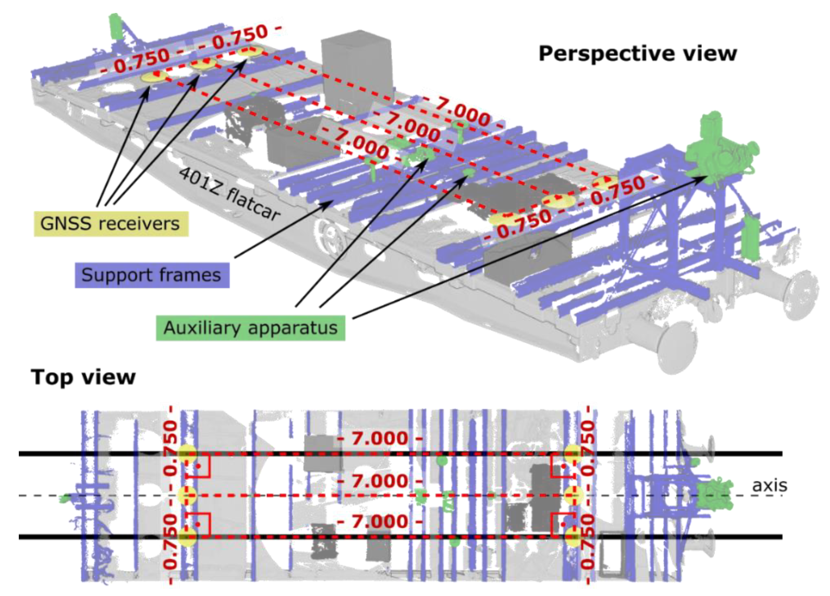
2.1. Railway Platform Configuration

The determination of geometrical parameters of the railway track, with particular emphasis on the track axis, was one of the main tasks of the research project InnoSatTrack. Information on the position was provided by six GNSS receivers which recorded raw satellite data with a frequency of 20 Hz, and for one campaign, with a frequency of 100 Hz. Readings from other sensors, e.g., inclinometers, inertial units, or optical cameras, were used in procedures of reduction of the GNSS receivers’ coordinates to the ground-level track axis, especially on curves and transition curves, where track superelevations occur [39].

GNSS receivers and other sensors used in the measurement campaigns were located according to the fixed design configuration. The distance between two kingpins on the railway platform 401Z equals 7000 mm [40]. Receivers were mounted on the platform in two parallel lines with two central receivers above kingpins above the track axis. The remaining four receivers were positioned above the rails perpendicularly to the direction of the track axis. Given the standard Polish track gauge of 1435 mm and the distance between the railhead axes equal to 1500 mm, the external receivers were located with an offset of 750 mm from the central receivers. The configuration of the sample railway platform used in one of the InnoSatTrack measurement campaigns is presented in Figure 1.

The point cloud presents six GNSS receivers marked in yellow mounted on the platform in a fixed configuration. The geometrical conditions include right angles in vertices and defined offsets between receivers. The remaining sensors used in the measurements are related spatially with receivers in one local coordinate system of the platform. In the case of the configuration presented in Figure 1, both the mobile laser scanner and the inertial unit components were located along the axis of the platform.

2.2. Stationary Scenario Field Works

Six Trimble R10 GNSS receivers mounted on tribrachs were attached to tripods. The re-creation of the geometrical configuration of GNSS receivers from the railway mobile platform was obtained using the tachymetric method. Trimble S7 robotic total station was set up on the Rybina point of the POLREF control network. Coordinates of the adjacent lower-order network control points for the instrument station tying (connecting) were obtained from the local department of cadaster and land surveying. Total stations’ 1” angular and 1.0 mm + 2.0 ppm linear errors produced millimeter stake-out errors. Also, the shape of the receivers’ distribution frame was controlled with certified linear measures, as was practiced in the railway campaign measurements.

Receivers were staked-out in two parallel lines with a distance of 7.000 m, representing along-track configuration on the platform. Cross-line offsets of receivers equaled 0.750 m. Also, the right angles between receivers’ positions were maintained in the final staked-out configuration consisting of front-line (left-front–LF, central-front–CF, and right-front–RF) and back-line (left-back–LB, central-back–CB, and right-back–RB) subgroups. Devices used in the field works are presented in Figure 2.

The bottom panel of Figure 2 presents a time series of GNSS static observations in six Trimble R10 receivers on 20 January 2021. The first session, Stat1, lasted for approx. 20 min. Three other sessions, Stat2, Stat3, and Stat4, lasted for approx. 30 min each. The synchronous recording of satellite observations with a frequency of 20 Hz was performed without major interference. A short break in the recording occurred in the RB receiver during the last 10 min of session Stat2.

The GNSS observations were post-processed using the Leica Infinity software. The calculation used synchronous satellite observations from the reference stations of geodetic active geodetic networks ASG-EUPOS and VRSnet.pl located in Gdańsk (GDSK), Elbląg (ELBL), and Braniewo (BRWO). The locations of the survey site (Rybina) and the reference stations are presented in Figure 3. Precise final orbits in SP3 files were downloaded from the IGS server.

2.3. Data Pre-Processing

The input data for the least-squares adjustment procedures are planar coordinates of six receivers calculated using projection functions. The first step to achieve this goal is the post-processing of raw satellite observations recorded by six used receivers and synchronous observations from adjacent CORS reference stations of active geodetic networks [30]. In the post-processing calculation, the final standard product 3 (SP3) generated by, e.g., GFZ or IGS [41], and GNSS receiver antennas’ parameters (ANTEX) [42] datasets are required to obtain the receiver’s coordinates in the WGS84 system [43]. SP3 final orbits contain the most accurate information on satellite positions that are interpolated from 15′ (IGS) or 5′ (GFZ) interval datasets.

Satellite measurements carried out in railway conditions are characterized by high frequency due to the need to present the geometry of the route with the shortest possible linear interval. For this purpose, the InnoSatTrack project used receivers measuring with frequencies of 20 Hz (Trimble R10 and Leica GS18) and 100 Hz (Trimble Alloy). The stationary measurement performed in this study used a frequency of 20 Hz to represent the conditions of the railway campaigns. However, one important factor related to the processing of satellite data should be noted. The SP3 product containing the data on satellite positions and satellite clock errors is provided every 15 min (IGS) or 5 min (GFZ). Hence, the estimated positions of receivers and other related geometrical parameters obtained are not fully independent between the epochs. This is a limitation of the study due to the unavailability of other methods for processing raw satellite data.

The second step of the initial stage of the calculations is the conversion of the Cartesian ellipsoidal Earth-centered Earth-fixed (ECEF) coordinates into curvilinear latitude and longitude coordinates using the Hirvonen algorithm [44]. Finally, in the third stage, the latitude and longitude are transformed into the Polish coordinate system PL-2000 [45], which is a modified Transverse Mercator projection [46]:

$$x_{TM}=k_{0}N\left[D+\frac{\left(1-T+C\right)D^3}{6}+\frac{\left(5-18T+T^2+72C-58e{{}^{\prime }}^2\right)D^5}{120}\right]$$

(1)

$$\begin{gathered} y_{TM}=k_0\left\{M-M_0+N\mathit{tan}\phi \left[D^2/2+\left(5-T+9C+4C^2\right)\right]D^4/24 \\ \hspace{1em}\hspace{1em}\hspace{1em}\hspace{1em}\hspace{1em}+\left(61-58T+T^2+600C-330e{{}^{\prime }}^2\right)D^6/720\right\}, \end{gathered}$$

(2)

where: $x_{TM}$, $y_{TM}$—Transverse Mercator planar coordinates, $k_0$—scaling parameter, $e{{}^{\prime }}^2=\frac{e^2}{\left(1-e^2\right)}$—second eccentricity, $N=a/{\left(1-e^2{\mathit{sin}}^2\phi \right)}^{1/2}$—prime vertical radius, $T={\mathit{tan}}^2\phi$, $C=e{{}^{\prime }}^2{\mathit{cos}}^2\phi$, $D=\left(\lambda -{\lambda }_0\right)\mathit{cos}\phi$—additional computation parameters, $M=a\left[\left(1-e^2/4-3e^4/64-5e^6/256\right)\phi -\left(3e^2/8+3e^4/32+45e^6/1024\right)\mathit{sin}2\phi +\left(15e^4/256+45e^6/1024\right)\mathit{sin}4\phi -\left(35e^6/3072\right)\mathit{sin}6\phi \right]$—true distance along the central meridian from the equator to the parallel $\phi$.

The Transverse Mercator projection ensures a low level of projection distortions through the introduction of narrow meridian zones. In the PL-2000 coordinate system, four zones with a width of 3° are used. The longitude of axial meridians λ₀ is 15° E, 18° E, 21° E, and 24° E. To distinguish the longitudinal coordinates in four meridian zones, the value of 500,000 m + (λ₀/3°) * 1,000,000 m is added to the eastern coordinate [47]. The datum of the PL-2000 system is not WGS84 but GRS80 [48]. The difference between the shape of the two ellipsoids is 1 mm in the length of the shorter polar semi-axis. Hence, the magnitude of corrections between GRS80 and WGS84 in the calculation of the PL-2000 system coordinates was treated as negligible.

The post-processed measurements carried out by six GNSS receivers either on the railway platform presented in Figure 1 or the stationary scenario presented in Figure 2 yielded WGS84 coordinates transformed into the PL-2000 planar system. In the next stage, three least-squares adjustment methods are applied to obtain estimates meeting the geometrical conditions of the platform frame.

2.4. Mathematical Model of Adjustment

The processing of geodetic and survey observations in certain cases includes specific relationships in the measured networks. A set of six GNSS receivers with defined linear offsets on the railway platform can be considered an example of such a network. Hence, fixed geometrical conditions applied in railway satellite measurements can be applied in the processing of recorded observations. The conditions-binded least-squares adjustment (CLS) takes the following form [49]:

$$\left.\begin{array}{c}\mathit{A}d\mathit{X}+\mathit{y}=\mathit{v}\\ \mathit{B}\mathit{d}\mathit{X}+\Delta =\mathbf{0}\\ \phi \left(d\mathit{X}\right)={\mathit{v}}^T\mathit{P}\mathit{v}=min\end{array}\right\}$$

(3)

where $\mathit{A}$ denotes the matrix of parameters, $d\mathit{X}$ denotes a vector of corrections to the estimated parameters, $\mathit{y}$ denotes the free term vector, and $\mathit{v}$ denotes the matrix of the corrections to observations. The four mentioned terms in the first line of Equation (3) are used in the standard (ordinary) least-squares (OLS) solution. Taking into account the fixed geometrical configuration matrices $\mathit{B}$ and $\Delta$ contain additional conditions binding the parameters. The term $\mathit{B}$ denotes the matrix of coefficients resulting from assumed conditions, $\Delta$ denotes the free term vector in conditional equations and $\phi \left(d\mathit{X}\right)$ denotes the objective function of the CLS adjustment that minimizes the sum of squares of the corrections to observations.

After minimizing the objective function $\phi$ replaced by the Lagrange function, the minimum value is defined [49]:

$$\frac{\partial {\phi }_L\left(d\mathit{X}\right)}{\partial d\mathit{X}}=2{\mathit{v}}^T\mathit{P}·\mathit{A}-2{\mathit{\kappa }}^T\mathit{B},$$

(4)

where $\mathit{P}$ denotes the observations weight matrix, and $\mathit{\kappa }$ denotes the correlates vector. Assuming a non-zero value of the determinant of the matrix ${\mathit{A}}^T\mathit{P}\mathit{A}$, the solution to Equation (4) is the estimator:

$$\widehat{d\mathit{X}}=-\mathit{Q}\left({\mathit{A}}^T\mathit{P}\mathit{L}-{\mathit{B}}^T\widehat{\mathit{\kappa }}\right),$$

(5)

where $\mathit{Q}$ denotes a variance-covariance matrix ${\left({\mathit{A}}^T\mathit{P}\mathit{A}\right)}^{-1}$. The value of the estimator $\widehat{d\mathit{X}}$ is determined by unknown correlates $\widehat{\mathit{\kappa }}$ when assuming that the estimator satisfies the conditions adopted in the adjustment task. After substituting the value of the estimator $\widehat{d\mathit{X}}$ into the matrix equation indicating the parameters in Equation (3) and assuming a non-zero determinant of matrix $\mathit{B}\mathit{Q}{\mathit{B}}^T$, the correlates vector takes the form [49]:

$$\widehat{\mathit{\kappa }}=-{\left(\mathit{B}\mathit{Q}{\mathit{B}}^T \right)}^{-1}\left(\Delta -\mathit{B}\mathit{Q}{\mathit{A}}^T\mathit{P}\mathit{L}\right),$$

(6)

With the correlated vector $\widehat{\mathit{\kappa }}$ determined, the $\widehat{d\mathit{X}}$, $\widehat{\mathit{X}}$, and $\widehat{\mathit{v}}$ terms are obtained. The conditions binding the estimated parameters (planar coordinates of the GNSS receivers on the platform) are represented in the adjustment algorithm by equations of the distance and angles between selected points (in this case, the receivers). Based on the fixed railway platform dimensions, linear-angular conditional relationships between the vertices of the survey figure (Figure 4) are formed.

The equations of the distance observations are functions of the approximate coordinates of the points. Due to the denominator’s square root operator used for distance calculation, these equations do not have a linear form. After expanding the equation into the Taylor series and limiting the sum to the terms of the first order, the following partial derivatives in relation to the coordinates of points I and K are obtained [50]:

$$\frac{\partial d_{\mathit{I}-\mathit{K}}}{\partial d{x}_{\mathit{I}}}=-\frac{x_{\mathit{K}}^o-x_{\mathit{I}}^o}{d_{\mathit{I}-\mathit{K}}^o}=-\cos \left(A{z}_{\mathit{I}-\mathit{K}}\right)$$

(7)

$$\frac{\partial d_{\mathit{I}-\mathit{K}}}{\partial d{y}_{\mathit{I}}}=-\frac{y_{\mathit{K}}^o-y_{\mathit{I}}^o}{d_{\mathit{I}-\mathit{K}}^o}=-\sin \left(A{z}_{\mathit{I}-\mathit{K}}\right)$$

(8)

$$\frac{\partial d_{\mathit{I}-\mathit{K}}}{\partial d{x}_{\mathit{K}}}=\frac{x_{\mathit{K}}^o-x_{\mathit{I}}^o}{d_{\mathit{I}-\mathit{K}}^o}=\cos \left(A{z}_{\mathit{I}-\mathit{K}}\right)$$

(9)

$$\frac{\partial d_{\mathit{I}-\mathit{K}}}{\partial d{y}_{\mathit{K}}}=\frac{y_{\mathit{K}}^o-y_{\mathit{I}}^o}{d_{\mathit{I}-\mathit{K}}^o}=\sin \left(A{z}_{\mathit{I}-\mathit{K}}\right)$$

(10)

where ($x_{\mathit{I}}$, $y_{\mathit{I}}$) and ($x_{\mathit{K}}$, $y_{\mathit{K}}$) denote the plane coordinates of points I and K, $A{z}_{\mathit{I}-\mathit{K}}$ denotes the azimuth of the line that is the angle measured clockwise from the northern X-axis towards the Y-axis. The superscripts (o) denote approximate values of the parameters.

The equations of the angle observations are formed similarly to the distance equations. An angle is the difference between two directions, C-L and C-R (right panel of Figure 4). The value of the angle at point C is determined by the difference between azimuths $A{z}_{\mathit{C}-\mathit{R}}$ and $A{z}_{\mathit{C}-\mathit{L}}$. The values of partial derivatives of the L, C, and R points obtain the following values [48]:

$$\frac{\partial {\alpha }_{\mathit{L}-\mathit{C}-\mathit{R}}}{\partial d{x}_{\mathit{L}}}=\frac{y_{\mathit{L}}^o-y_{\mathit{C}}^o}{{\left(d_{\mathit{C}-\mathit{L}}^o\right)}^2}$$

(11)

$$\frac{\partial {\alpha }_{\mathit{L}-\mathit{C}-\mathit{R}}}{\partial d{y}_{\mathit{L}}}=-\frac{x_{\mathit{L}}^o-x_{\mathit{C}}^o}{{\left(d_{\mathit{C}-\mathit{L}}^o\right)}^2}$$

(12)

$$\frac{\partial {\alpha }_{\mathit{L}-\mathit{C}-\mathit{R}}}{\partial d{x}_{\mathit{R}}}=-\frac{y_{\mathit{P}}^o-y_{\mathit{C}}^o}{{\left(d_{\mathit{C}-\mathit{R}}^o\right)}^2}$$

(13)

$$\frac{\partial {\alpha }_{\mathit{L}-\mathit{C}-\mathit{R}}}{\partial d{y}_{\mathit{R}}}=\frac{x_{\mathit{P}}^o-x_{\mathit{C}}^o}{{\left(d_{\mathit{C}-\mathit{R}}^o\right)}^2}$$

(14)

$$\frac{\partial {\alpha }_{\mathit{L}-\mathit{C}-\mathit{R}}}{\partial d{x}_{\mathit{C}}}=\frac{y_{\mathit{R}}^o-y_{\mathit{C}}^o}{{\left(d_{\mathit{C}-\mathit{R}}^o\right)}^2}-\frac{y_{\mathit{L}}^o-y_{\mathit{C}}^o}{{\left(d_{\mathit{C}-\mathit{L}}^o\right)}^2}$$

(15)

$$\frac{\partial {\alpha }_{\mathit{L}-\mathit{C}-\mathit{R}}}{\partial d{y}_{\mathit{C}}}=-\frac{x_{\mathit{R}}^o-x_{\mathit{C}}^o}{{\left(d_{\mathit{C}-\mathit{R}}^o\right)}^2}+\frac{x_{\mathit{L}}^o-x_{\mathit{C}}^o}{{\left(d_{\mathit{C}-\mathit{L}}^o\right)}^2}$$

(16)

The partial derivatives of the equations representing the distance and angle observations are used in the coefficient matrix $\mathit{A}$ and the conditional matrix $\mathit{B}$ presented in Equation (3). The final result of the CLS adjustment is the set of estimators of receivers’ coordinates. In reference to the main working thesis of the research project InnoSatTrack, the obtained adjusted coordinates of the receivers will be reduced according to the readings of the other sensors (e.g., inclinometers) and, after the necessary reduction to the ground level, will indicate the location of the railway track axis with higher accuracy.

Results of the CLS adjustment were compared in the set of stationary scenario coordinates with results of two other methods, standard OLS adjustment and robust adjustment (RLS) with Huber damping function applied. Robust estimators are calculated iteratively using the following formula [51]:

$${\mathit{X}}^j={\left[{\mathit{A}}^T\mathit{w}\left({\mathit{v}}^{j-1}\right)\mathit{A}\right]}^{-1}{\mathit{A}}^T\mathit{w}\left({\mathit{v}}^{j-1}\right)\mathit{y},$$

(17)

where $j$ denotes the step of the iterative solution of the estimation, $\mathit{w}\left({\mathit{v}}^{j-1}\right)$ denotes the diagonal matrix of the Huber weight function:

$$w\left(v_i\right)=\left\{\begin{array}{ccc}{p}_i& for& \left|{\overline{v}}_i\right|\le t\\ \frac{t}{\left|{\overline{v}}_i\right|}{p}_i& for& \left|{\overline{v}}_i\right|>t\end{array}\right.,$$

(18)

where $v_i$ denotes observational correction to the $i$-th observation, ${\overline{v}}_i$ denotes the standardized observational, and $t$ denotes the Huber function threshold parameter.

3. Results

The section was divided into three parts, presenting the results of three adjustments methods used in the study (Section 3.1), compliance of obtained estimates with the local planar coordinate system (Section 3.2), and analysis of maintenance of the initial theoretical shape of railway platform frame (Section 3.3).

3.1. CLS, OLS, and RLS Adjustment

The result of the post-processing stage was obtaining 24 time-tagged lists of GNSS receiver coordinates. UTC enabled synchronization of the records for each epoch of four static sessions. The procedure was not provided in the post-processing software and required the creation of custom software. The initial aim of the field survey campaign was to collect 100,000 epochs of synchronous positions of six receivers. Dataset was to provide a sufficient sample representing various satellite configurations and receiver-dependent errors during the railway dynamic measurement campaign. Due to the break in the recording in session Stat2, the final cardinality of the set was 96,729 observations (21,855 in Stat1, 16,694 in Stat2, in Stat3, and 29,742 in Stat4). 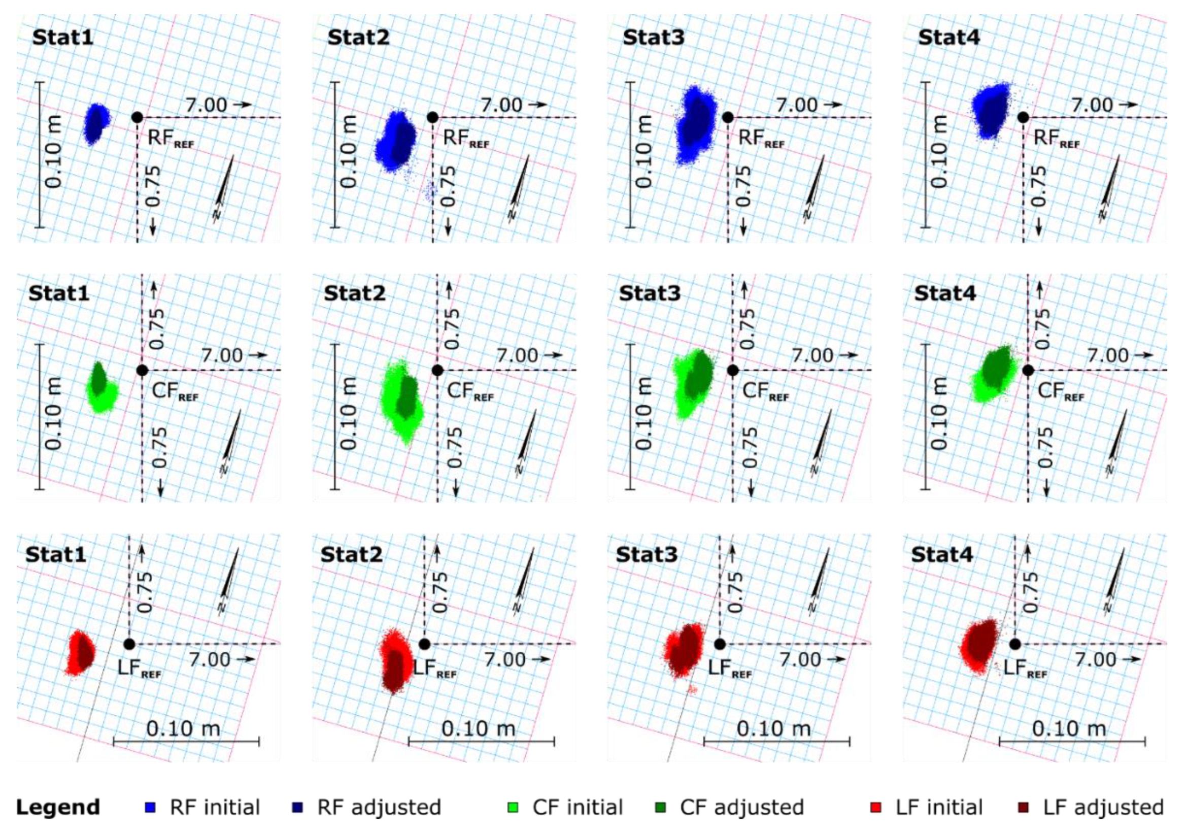Figure 5 and Figure 6 present the results of the post-processing of four static sessions.

The colors representing six GNSS receivers correspond to the time series presented in Figure 2. Fixed linear dimensions used in the railway platform were added to the figures to highlight the outliers recorded during the field campaign.

Three compared LS-adjustment methods were applied on the sets of synchronous coordinates of six receivers from each GNSS-measurement epoch. Standard OLS adjustment includes equations describing relations between z- and y-coordinate parameters. Robust RLS estimation introduces the iterative procedure, including weight-dependent observational corrections. The algorithm of the CLS adjustment yields estimators that satisfy the geometrical assumptions of the railway platform frame recreated in the case of this study by receivers staked out on tripods in the field. An example of the result of adjustment with parameter-binding conditions is presented in Figure 7.

The initial positions from the post-processing of six receivers are marked with circles. The CLS estimators of the receiver positions are marked with crosses. The figure presents an atypical case of epoch with the outlier position of the left-front (LF) receiver. The red arrow indicates the correction applied by conditions-based CLS adjustment. The right panel of the figure contains control quantities computed based on the adjusted coordinates. The presented distances and angles indicate that estimators comply with the design fixed dimensions of the platform frame shape.

Three algorithms of OLS, RLS, and CLS adjustments were applied to 96,729 sets of synchronous observations. In order to illustrate the result, the initial (unadjusted) and CLS-adjusted observations are presented in Figure 8 and Figure 9. The observations before and after the adjustment are marked with lighter and darker color shades, respectively. Horizontal panels with different colors refer to six GNSS receivers. The results obtained for four individual static sessions are presented in the columns. Each panel contains the reference position of the receivers in the PL-2000 coordinate system determined by the tachymetric method.

The most precise initial (post-processed) coordinates were obtained in static session Stat1. The least precise results occurred in session Stat3, especially in the case of the LB receiver (top panel of Figure 9). The CLS estimation resulted in a decrease in the subsets’ standard deviation values. Part of the estimates of the coordinates of the frame back-line receivers was significantly affected by the anomalous LB receiver coordinates.

The next stage of the study was the comparison of initial receivers’ coordinates from post-processing and coordinates calculated using ordinary (OLS), robust (RLS), and conditions-binded (CLS) least-squares estimation. Static sessions’ data processing yielded four independent sets of estimated coordinates of the GNSS receivers. Coordinates were averaged with standard deviations and are presented in

Table 1. Standard deviations of initial, OLS-, RLS-, and CLS-adjusted coordinates.

ID	Init		OLS		RLS		CLS
	dx [mm]	dy [mm]	dx [mm]	dy [mm]	dx [mm]	dy [mm]	dx [mm]	dy [mm]
LF	3.0	6.9	4.0	6.5	5.9	5.7	6.2	4.4
CF	7.2	2.5	8.3	3.9	6.7	4.1	6.3	4.2
RF	8.1	2.9	6.7	2.9	6.5	3.2	6.4	4.1
LB	10.9	4.9	10.9	4.3	6.0	3.9	4.3	4.0
CB	3.7	4.5	1.7	4.5	3.8	4.1	4.4	3.9
RB	6.0	5.8	7.7	4.5	5.6	4.5	4.4	3.7

.

Standard deviations of both the initial (unadjusted) and OLS-estimated coordinates yielded a maximum value of 10.9 mm and a mean value of 5.5 mm. The maximum and mean values of standard deviations were reduced to 5.0 mm and 6.7 mm (RLS) and 4.7 mm and 5.0 mm (CLS). However, it should be noted that obtained smaller values do not necessarily satisfy, in all cases, the condition of nominal geometrical relationships of the survey frame.

3.2. Control Network Impact Analysis

An important issue related to the processing of GNSS-derived railway track coordinates is relating the satellite measurements with a railway surveying control network. Obtained spatial data, after proper harmonization [52], are stored in numerical maps for further use, e.g., in the maintenance of the track. The quality of the control network along the railway track is not constant and includes points of various network orders. In this study, one POLREF point and two adjacent lower-order points were used. Coordinates of receivers in the planar PL-2000 coordinate system were determined using the total station and compared with coordinates from post-processing and LS adjustments (

Table 2. Differences in the initial and LS-adjusted receiver coordinates in relation to the reference.

ID	Init		OLS		RLS		CLS
	dx [mm]	dy [mm]	dx [mm]	dy [mm]	dx [mm]	dy [mm]	dx [mm]	dy [mm]
LF	−12.0	−19.8	−12.6	−21.5	−13.4	−21.9	−12.7	−21.6
CF	−19.8	−20.0	−11.9	−20.0	−14.2	−19.1	−12.2	−20.8
RF	−9.5	−22.3	−11.9	−20.9	−11.3	−22.4	−11.7	−20.1
LB	−3.2	−18.6	−13.2	−19.7	−9.1	−20.2	−13.0	−19.9
CB	−12.5	−19.5	−12.4	−19.2	−11.9	−20.0	−12.5	−20.1
RB	−14.4	−16.9	−13.5	−21.2	−14.0	−19.4	−13.0	−20.4
Mean	−11.9	−19.5	−12.6	−20.4	−12.3	−20.5	−12.5	−20.5
StDev	5.0	1.6	0.6	0.8	1.8	1.2	0.5	0.6

).

Three LS-adjustment methods used coordinates from post-processing calculation. Hence, the shifts of positions of receivers related to the reference coordinates were similar, which was represented by mean values. The factor that was changing was the standard deviation indicating the degree of distribution of points. Standard deviations of differences of coordinates exceeded the 1 mm threshold in the initial (unadjusted) and RLS datasets, with the greatest values in the north-south direction of the X-axis. At this stage, the OLS-, and CLS-adjustments results show similar quality reducing the precision of receivers x- and y-coordinates to 0.6 mm and 0.8 mm, and 0.5 mm and 0.6 mm, respectively.

Differences for six receivers of approximately −1.2 cm (the x-coordinate) and −2.0 cm (the y-coordinate) indicate the presence of a systematic error related to the control network. Significantly smaller standard deviations show high repeatability of measurements. The tachymetric method ensures local station-related accuracies of single millimeters. However, the quality of the control network determines the final accuracy in the used reference frame. The control network point coordinates were not determined in the study but were provided by the local administration cadastre and land surveying department. A potential cause of obtained differences according to the reference coordinates can be the different implementation of ETRF (ITRF) in control networks of different orders.

The presence of systematic errors in the results indicated the importance of the factor of control network quality. As the processed satellite observations may yield coordinates with high precision, it does not imply compliance with the local realization of the used reference frame. The importance of this conclusion is even greater, taking into account the dynamic measurements in the mobile railway platform. The local density of points and coordinates quality affect the harmonization of GNSS processed data with the railway numerical maps.

3.3. Frame Geometrical Analysis

The principal assumption of the research project was the constant configuration of six GNSS receivers. The frame consisted of fixed distances and right angles between the receivers’ positions. In this subsection, the distances and angles calculated from averaged initial and LS-adjusted coordinates are compared with theoretical values from the frame.

Table 3. The differences in distances in relation to the theoretical frame fixed values.

Distance	D ref [m]	dD init [mm]	D OLS [mm]	dD RLS [mm]	dD CLS [mm]
LF-LB	7.000	2.1	4.0	1.3	−0.1
CF-CB	7.000	1.9	1.3	−0.8	−0.1
RF-RB	7.000	4.4	2.5	2.8	−0.1
LF-CF	0.750	−7.7	−8.8	−1.8	0.0
CF-RF	0.750	10.3	11.9	3.5	0.0
LB-CB	0.750	−9.3	−9.4	−3.3	0.0
CB-RB	0.750	−2.1	−2.1	−1.8	0.0
LF-RF	1.500	2.5	3.1	1.7	0.0
LB-RB	1.500	−11.4	−11.6	−5.1	0.0
LF-RB	7.159	0.5	0.9	1.0	−0.1
LB-RF	7.159	4.0	3.7	2.2	0.0
	mean |dD|	5.1	5.4	2.3	0.0

presents the distance analysis, and

Table 4. The differences in angles in relation to the theoretical frame fixed values.

Angle (L-C-R)	α ref [°]	dα init [“]	dα OLS [“]	dα RLS [“]	dα CLS [“]
CF-LF-LB	90	633.6	−13.9	−574.1	−0.9
LF-LB-CB	90	−701.8	−734.9	−1.1	0.9
RB-RF-CF	90	−190.0	−207.9	−944.5	−5.7
CB-RB-RF	90	−514.8	−112.8	−35.1	5.7
RF-CF-LF	180	−854.2	−209.0	1320.4	6.6
RB-CB-LB	180	−1627.3	−1278.5	−234.4	6.6
	mean |dα|	753.6	426.2	518.3	4.4

presents the angle analysis.

The theoretical assumptions of the receiver positioning during the stationary survey corresponded to the target configuration used during mobile survey campaigns conducted on railway routes. The reference distances between six receivers (D _ref) correspond to Figure 1, presenting a typical sensor configuration on the mobile railway platform. Reference distances represent the main along-and cross-track directions and two platform frame diagonals. The third column (D _init) contains the differences values with respect to the reference distances. The remaining three columns present the differences obtained from the coordinates of three compared LS adjustment methods.

The distances calculated from the initial coordinates from post-processing in two cases exceeded the 1 cm threshold value. The mean average distance difference equaled 5.1 mm and 5.4 mm in initial and OLS datasets, respectively, which showed that the application of standard LS adjustment did not improve the compliance of the estimates with theoretical platform frame configuration. The mean value was reduced twice to 2.3 mm in robust RLS adjustment, however, in three cases the differences exceeding 3 mm were noted. Differences with a mean value not exceeding 0.1 mm were obtained in conditionally-restricted CLS adjustment, which met the principal geometry of the receivers’ frame.

The differences in angles calculated from the initial coordinates significantly differed from the reference values and, in one case, reached 1627.3”, which corresponds to 0.45°. OLS and RLS adjustment methods did not eliminate the discrepancy between the calculated geometry and the fixed platform frame. Mean absolute values of angle differences equaled 0.12° and 0.14° for OLS and RLS methods, respectively. A major improvement in the estimates of the receivers’ geometry was obtained by CLS adjustment, where the mean absolute value equaled 4.4”, which corresponds to 0.001°.

The conducted analysis showed superior applicability of the conditions-binded CLS method to the standard OLS and robust RLS method. Theoretical assumptions maintaining the fixed geometrical principle of the railway platform in distances and angles were satisfied only in CLS adjustment. On every six-receivers measurement epoch, the coordinates estimates met the design requirement.

4. Summary

The aim of the study was the applicability assessment of three estimation methods in the adjustment of coordinates of six GNSS receivers distributed within a defined geometric configuration. Three least-squares methods were tested to mitigate random errors: ordinary least-squares (OLS), robust estimation (RLS), and adjustment with conditions binding parameters (CLS). The configuration used on the railway survey platform was re-created in the field on tripods using the precise tachymetric method. The site was chosen in the vicinity of the POLREF control network point. Six Trimble R10 GNSS receivers in four static sessions recorded 96,729 synchronous observations with a frequency of 20 Hz.

The results were analyzed in terms of enhancement of precision, compliance with coordinates of the PL-2000 system, and meeting the geometrical criteria of the fixed frame used both in the railway platform and in the field test site. Gaussian standard deviation with 1σ degree of freedom was used for the assessment of changes in precision in the initial (unadjusted) dataset and three least-squares processed sets. Standard deviations in four static sessions showed a similar mean value of 5.5 mm in initial post-processed and OLS datasets. Values of 5.0 mm and 4.7 mm were obtained in RLS and CLS adjustments indicating improvement in precision using those methods.

Analysis of coordinates determined using tachymetry showed the presence of systematic linear error in all LS-adjusted results. A significant reduction of precision was noted in OLS and CLS methods compared to the initial data. Analysis shows the impact of local control network quality and the necessity of assessing that factor during dynamic railway measurements. The final analysis was focused on maintaining the fixed geometry between estimators obtained in three LS methods. The initial dataset gave a mean linear error of 5.1 mm in 11 analyzed frame distances. Standard OLS adjustment did not improve the result and obtained a mean error of 5.4 mm. Values of 2.3 mm and 0.0 mm were obtained in RLS and CLS methods, respectively. Distance analysis showed that conditions-binded CLS estimation maintains the linear dimensions of estimates.

Analysis of angles in the estimate sets covered 6 angles of 90° and 180° in vertices of the platform frame. Comparison of reference angles with angles calculated from adjusted coordinates yielded obtaining the greatest error in an unadjusted dataset with a mean value of 0.21°. Slight improvement of the angular conditions occurred in OLS and RLS adjustments where errors of 0.12° and 0.14° occurred, respectively. Similarly to the distance errors analysis, the CLS method obtained the smallest mean error of 4.4” that shows meeting the geometrical conditions of the railway platform frame.

Performed field tests and analysis showed that the conditions-binded CLS is a more applicable solution than OLS and RLS adjustment methods. CLS estimates maintain the geometrical topology of the frame used for GNSS receivers’ installation in railway measurements. The RLS method obtained linear errors of several millimeters and angular errors of several arc minutes relative to the theoretical platform frame, which places it in second place in the list of methods of alignment of satellite data. Hence, the CLS is recommended for application with the post-processed satellite data from receivers in the InnoSatTrack project.