1. Introduction
With the development of big data and computer hardware, it has become possible to train large deep neural networks (DNNs). Therefore, deep neural networks have been widely studied in recent years and applied to face recognition, image classification, autonomous driving, natural language processing, and other artificial intelligence fields. Although deep neural networks have excellent performance and have been able to lead humans in some tasks, most deep neural network models have the disadvantages of large size (large space consumption for model storage) and high computational cost.
The excellent performance of deep neural networks comes at the cost of high computational complexity and huge memory consumption. As the network grows in size, the number of parameters in the network grows and the amount of computation becomes larger. This leads to two core problems:
It is difficult to deploy it in some resource-constrained devices, which greatly limits the application scenarios of neural networks. For example, in scenarios such as the Internet of Things (IoT), embedded systems not only lack rich computing and storage resources but also have a very urgent need for low power consumption.
It is difficult to apply in some industrial scenarios with high real-time requirements, such as autonomous driving. These technologies require extremely high real-time network inference; otherwise, there will be safety hazards.
Therefore, a variety of deep neural network compression and acceleration techniques have emerged to try to remove redundancy in the network while ensuring network accuracy, i.e., to find a good tradeoff between network performance and computational cost.
In general, model compression and acceleration of deep neural networks have both industrial application and academic research implications: In terms of application, the technology can make it easier to land artificial intelligence applications. Current deep neural networks are difficult to use in scenario-constrained environments due to their large number of parameters and computations, and studying how to compress and accelerate deep neural networks will help solve such problems. In theoretical research, the technique can help people to better understand deep neural networks. Various existing deep neural networks all suffer from information redundancy. By using model compression and acceleration algorithms, the redundancy in the network can be removed and the part of the network that really works can be uncovered. The study of this part will help people directly design deep neural networks that are more efficient and have better generalization ability.
Previous methods could be roughly divided into two categories. The first category is to design a lightweight network structure. Taking MobileNet [
1], SqueezeNet [
2] ShuffleNet [
3], and DenseNet [
4] as examples, the main idea of these methods is to design a more efficient network computing method to reduce network parameters without decreasing network performance; however, although the lightweight models could effectively reduce network parameters, their generalization abilities are partly sacrificed and perform more poorly than conventional models. For example, the lightweight model MobileNet-224 achieves 70.6% accuracy on the ImageNet classification, but a non-conventional model such as SENet obtains 83.8% accuracy. It motivates us to seek new mechanisms for achieving compressed models. The second class quantizes the weights and input of a CNN from a 32-bit float number to a lower-bit number. This paper mainly studies the method for quantification.
This paper focuses on the study of 8-bit quantization with minimal accuracy loss. According to the traditional quantization method, the post-training quantization method based on clipping is proposed. Firstly, the weight information and the floating-point number of the input data flow are clipped to a fixed-point range in the training, which can not only avoid the search and calculation of the range of the input data flow in the dynamic quantification process but also greatly reduce the amount of calculation. Moreover, the loss caused by the clip operation in the training process can be compensated by the Lq loss we proposed during model training. It penalizes the differences between clipped weights and non-clipped weights for diminishing the performance drop. Then, the model is converted to 8-bit for inference. Our approach is simple but effective in compressing the model while maintaining its performance. To validate the effectiveness of the proposed method, it is conducted on YOLO V3 and Faster R-CNN model for object detection on the PASCAL VOC benchmark dataset. Performances demonstrate that our model could compress the model to 18.84% without losing the accuracy of detection, and the speed is increased by about 381%.
The contributions of our work are three folds:
A clipping-based post-training 8-bit quantization method is proposed, which can reduce the calculation amount in the traditional quantification method and reduce the accuracy loss.
A method using singular value decomposition (SVD) in the full connection layer is proposed, which can effectively reduce the redundant parameters and improve the training speed.
An Lq loss is proposed to reduce the accuracy loss caused by clipping during training in this training–clipping method.
In the next section, we present some of the outstanding work in the field of quantification and explain the excellence of our approach. In the third section, we will introduce the previous int8 quantization methods and their problems. The fourth section will elaborate on our methods and their advantages. In the fifth section, we will verify the superiority of the clipping-based method in the mainstream object detection network. There is a discussion section about the limitations and future developments, and the last section will summarize the contributions of this paper.
2. Related Work
According to the degree of low precision, network quantization can be further divided into ultra-low precision quantization and 8-bit quantization. Ultra-low precision quantization refers to the use of 1 to 4-bit values to replace 32 floating-point parameters in the source network. A representative work of ultra-low precision quantization is the binary quantization network (BNN) [
5]. When training the neural network, BNN quantizes the network weight parameters and activation values to 1 or −1, so the exclusive OR (XOR) operation in the logical operation can be used to replace the matrix multiplication and addition operation of the original network, which greatly improves the operation efficiency. A three-valued quantization network (TWN) [
6] quantizes ownership values to −1, 0, and 1. Incremental quantization network (INQ) [
7]: By iterative logarithmic transformation of weight parameters, the quantization error of each iteration is reduced, and finally the network performance degradation caused by the quantization process is reduced. However, due to the ultra-low precision quantization, the precision of the network performance is usually negatively affected. Moreover, the training error fluctuates violently in the training process. The most commonly used quantization method in the industry is 8-bit quantization. Its quantization strategy is relatively conservative. Using an 8-bit fixed-point number to store and calculate network parameters has little effect on network accuracy.
Recently, to solve the problem of accuracy loss and instability in the simulation quantification, work such as that of [
8] carried out the theoretical analysis of the convergence stability of quantitative training, and based on this, proposed the error-sensitive learning rate adjustment and the direction-adaptive gradient truncation method. Dettmers proposed a fixed-point method using single instruction multiple data (SIMD) operations to improve model performance [
9]. Zhu F. et al. established a unified 8-bit (Int8) training framework for general convolutional neural networks, which can accurately and efficiently train various networks and tasks. A direction-sensitive gradient clipping technique to reduce the gradient direction deviation and a deviation back learning rate scaling technique to avoid illegal gradient updating along the wrong direction were also proposed [
10]. Jacob B proposed a quantization scheme, which only depends on an integer algorithm to approximate the floating-point calculation in neural networks. The training the of simulation quantization effect helps to recover the accuracy of the model to almost the same level as the original data [
11].
Some well-known methods of 8-bit quantization are introduced above, but recently there have been some novel quantization methods that can be referred to and compared. Peng proposes an optimization method based on the idea of quantization compensation [
12]. Compared with their work, we design a new loss function to compensate for clipping loss, which can avoid model bias. Bao proposed a clipping method based on learning parameters to quantize the network parameters during the training phase [
13], while our method performs clip processing before training and then quantifies the inference, which is more efficient and has less final accuracy loss. Gheorghe also proposes a quantization method for adaptive models [
14], but the author’s method of improving model efficiency by removing the fully connected layer leads to a large loss of information, while our processing of the fully connected layer using SVD can refine the effective information with higher accuracy. Ullah’s method also quantifies by weight intervals [
15]. However, the author’s method was only validated on shallower networks such as VGG, and its processing of only valid bits may lead to accuracy loss in deeper networks.
3. Preliminary Knowledge
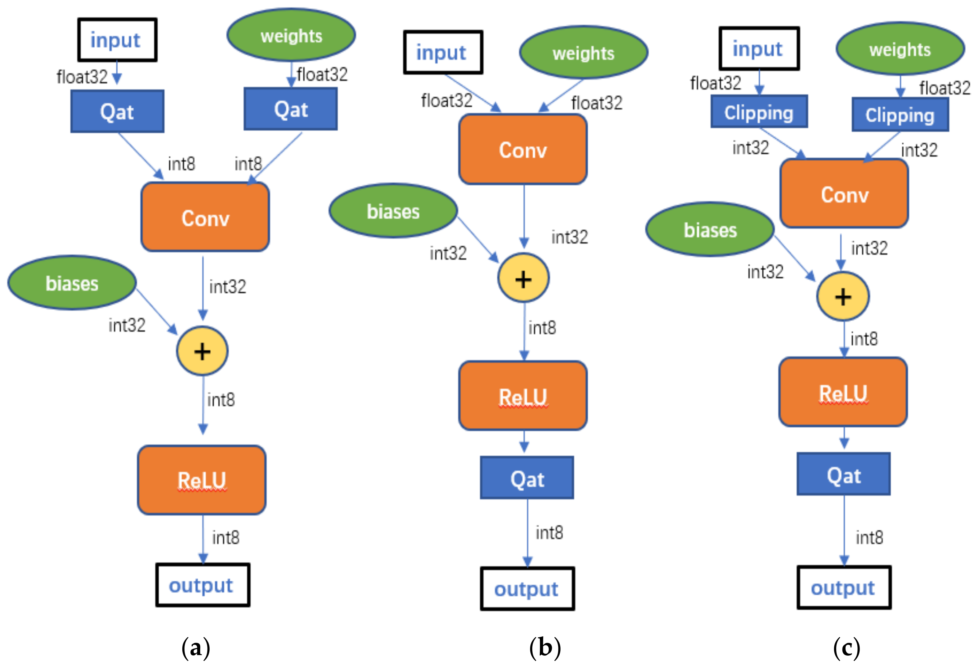
The process of quantization is the process of converting floating-point numbers into fixed-point numbers, and it is also the process of changing from continuous values to discrete values. The quantization methods are generally divided into training-aware quantization and post-training quantization, as shown in
Figure 1a,b, and
Figure 1c briefly illustrates the clipping-based post-training quantization method that we propose.
The basic ideas of the three strategies in
Figure 1 are as follows.
- (a)
Training quantization: The model is directly quantized, and the input and weights are converted to 8-bit numbers during model training. At last, inverse quantization is performed during model inference.
- (b)
Post-training quantization: The model is still trained with 32-bit floating point numbers, and the weight distribution is obtained to derive the quantization parameters, and finally the quantized model is deployed in the inference stage.
- (c)
Clipping-based post-training 8-bit quantization: The weights and inputs are clipped before training so that they are trained as 32-bit fixed-point numbers, and then the quantization model is deployed to the inference stage.
This is only a brief description of the method. The details of the operational mechanism, formulae derivation, and strengths and weaknesses analysis will be described later in
Section 3.1,
Section 3.2, and
Section 4.1.
Next, we analyze the defects in training-aware quantization and post-training quantization methods.
3.1. Training-Aware Quantization
Training-aware quantization conducts quantization during training. It uses floating-point numbers to save fixed-point parameters during training and uses fixed-point parameters directly during the final inference. The quantization parameters in the network are learned and updated during the training process.
The forward propagation of quantization during training is as follows. It first multiplies the input x and weight w by the scale and then converts it to
and
through the round function for calculation (formulas (1) and (2)):
In backpropagation, since
is a discrete value, the second term in (formulas (3) and (4)) is non-derivable. To solve this problem, researchers proposed a straightforward estimator [
16] (STE), as shown in
Figure 2. The stepwise function in
Figure 2 represents a common uniform quantization method, and its gradient is normally difficult to find. STE is actually a sign function that takes 1 when the gradient of the stepwise function is greater than or equal to 0, so that the gradient here can be regarded as 1. By doing so, the quantization function becomes an identity mapping f(x) = x for backpropagation.
In short, the discrete values in the neural network will lead to a performance drop, caused by its low number of bits. Moreover, the inherent discrete nature of the quantized model hinders the conventional backpropagation calculations, which assume the weights are continuous. Although mandatory fitting methods could train a model in a discrete manner, it makes the training unstable.
3.2. Post-Training Quantization
Post-training quantization refers to the quantization of model parameters after training when the weights of the model are fixed. Generally, the quantization parameters that minimize the quantization loss of each layer of the network are obtained through the validation set. The quantization process could be generally divided into dynamic quantization and static quantization.
- (1)
Post-training dynamic quantification
This method is to quantize the operations after the convergence of the floating-point model training, where the weights are quantized in advance. The activation output needs to be dynamically quantified in the forward propagation process during inference. During quantization, each layer calculates a quantization parameter to obtain the maximum and minimum input and then quantizes them. In the actual calculation process, each layer needs to be traversed, which increases the calculation cost.
- (2)
Post-training static quantification
The weights are quantized in advance in this method. Moreover, the activation output is quantized based on the fixed quantization parameters recorded in the small sample calibration process (the maximum and minimum values of each layer). There is no recalculation of quantization parameters in the whole process, so the computational cost is low However, the risk of accuracy drop is relatively high because small samples often cannot accurately reflect the data distribution and data range of the whole dataset.
Taking our commonly used uniform linear quantization as an example, we briefly describe the traditional post-training quantization method. Assuming that the weights of convolution are w, the input is x, and the weight quantization parameters obtained in advance are
and
, the input quantization parameters are
. Formulas (5) and (6) show the process that input and weights are linearly adjusted to (−1, 1):
The normalized input
and weights
are multiplied by a magnification S and rounded to an integer (if
is 128, then the new
and
are converted to int8):
The core of the convolutional neural network is the matrix multiplication of
and
. In the following, we use a series of dequantization operations to simplify this multiplication. Formulas (7) and (8) are obtained from formulas (5) and (6):
Multiply formulas (7) and (8):
Since
,
,
,
are known constants, the formula is simplified with
,
,
,
:
In short, the calculation of training-aware quantization is complex and requires a long training time. As for the dynamic post-training quantization, the range of dynamic statistical input is needed, the amount of calculation is large, and the computational complexity of inverse quantization is high. For static post-quantization, the clip value obtained by small samples cannot fully reflect the data distribution of the whole dataset, which inevitably leads to accuracy loss. Therefore, in the next section, we propose a simple and efficient quantitative method with little accuracy loss.
3.3. Object Detection Networks
At present, object detection algorithms based on convolutional neural networks can be divided into two categories: one-stage object detection and two-stage object detection algorithm. The one-stage object detection algorithm is based on convolutional networks. The feature map directly returns the location of the target, and the model further classifies the target categories. The representative works are SSD [
17] and YOLO [
18,
19,
20,
21] series. In two-stage target detection algorithms, the first stage is to generate region proposals, and the second stage is to return to the target location and classify the target category based on the regional proposal, which is represented by the R-CNN [
22] series algorithms, including R-CNN, Fast R-CNN [
23], Faster R-CNN [
24], and mask R-CNN [
25]. This paper takes a one-stage mature representative network, YOLOv3, and a two-stage representative network, Faster R-CNN, for validating the effectiveness of our designs The process and experimental design of the clipping-based post-training 8-bit quantization method are shown in
Figure 3. As shown in
Figure 3, we apply our clipping base quantization method to two representative one-stage, two-stage target detection networks. After fine-tuning, we check whether the accuracy loss meets the expectation, and if the accuracy still decreases, we adjust the loss function considering the loss of clipping operation to obtain the result.
4. Method
Usually, the neural network model takes 32-bit single-precision floating-point numbers as parameters. The floating-point number consists of three parts: symbol (one bit), exponential (eight bits), and tail numbers. The pipeline of floating-point addition and subtraction includes: (1) Checking the 0 operands. If the number of operations involved is zero, the operations directly return the results. (2) Comparing the size of two order codes and completing the alignment for the addition or subtraction of the tail number. (3) The results are rounded and standardized. When the network size is large, it requires a lot of memory and computational resources to conduct the floating-point operation. Differently, the low-precis fixed-point operation could save memory and compute, because it computes the summation directly; it is needless to conduct alignment before computing. Network quantification is based on this idea. It transfers the number from floating points to fixed points by discretization of the weight parameters of the network. It effectively compresses the storage space of network parameters and reduces the amount of calculation. Specifically, it uses a low-precision way to store and calculate network parameters. Usually, the neural network uses 32-bit floating-point number to store all the parameters and calculation results of the network. If a small amount of network performance is sacrificed, the data are mapped to a smaller numerical range by using the quantitative method, which can greatly reduce the number of parameter storage and the memory space occupied by calculation. By adopting a reasonable low-precision method, only a small part of network precision can be lost while the model volume is greatly compressed.
To reduce the model and solve the excessive accuracy loss caused by traditional quantification methods, we propose a post-training quantization method combined with a clip during training. In addition, a fully connected layer compression method based on singular value decomposition is conducted to minimize storage consumption. Furthermore, we propose a new loss function to improve the accuracy and avoid the performance drop during quantization. These methods have achieved good results in the following experiments in
Section 4, and their mechanism will be sequentially introduced as follows
4.1. Clipping-Based Post-Training Quantization
The key to this method is to clip input and weights during training. The clipping process will inevitably bring some accuracy drop. Differently from the traditional method, we clip the input to a fixed range in the training process. During the training of the model, the input learning of each layer can make up for a certain accuracy loss caused by clip operation to the greatest extent. Moreover, after clipping to a fixed range, we will know the maximum and minimum values of each layer parameter in each calculation process. It is helpful to avoid the cyclic calculation process of searching the range of input data stream dynamically, and we can also ensure that the range of input values is fixed in the range of our clip in order to avoid the risk of accuracy drop of post-training static quantization.
The calculation method is as follows. We first clip the input and weight to
, where j and k are integers:
Similarly, the input and weight are converted into int8 type by multiplying an amplification factor and round function:
Next, the dequantization process is also very simple (as shown in
Figure 4):
Figure 4 shows a simplified forward propagation process for neural networks. Combined with Equations (16)–(19), it shows that the computational effort in forward propagation can be saved by multiplying the quantization parameters. This ingenious combination avoids many redundant parameter calculations. By comparing formula (18) with formulas (11)–(13), we can find that we have saved a lot of computation in the process of inverse quantization. In short, our post-training quantization method combined with clip during training has obvious advantages in avoiding the huge amount of calculation in dynamic post-training and solving the problem of accuracy loss in static post-training.
It is worth mentioning that the clip values of our training–clipping method are symmetrically centered on 0 and are the integer power of 2; this minimizes the amount of computation with the representation of int8, but the closer the value of the clip to the real data range, the smaller the accuracy loss. In the experiment in
Section 4, we will comprehensively consider these effects to obtain the best quantitative results.
4.2. Decomposition of Fully Connected Layers
Singular value decomposition (SVD) is a widely used algebraic feature extraction method in the field of machine learning [
26]. Singular value decomposition (SVD) is to decompose a linear transformation into two linear transformations, one representing rotation and one representing stretching.
In the object detection network, most of the classification results or prediction results need to be processed through the fully connected layer. The fully connected layer generally has a large number of parameters. In this paper, the first-order input with the size of 1024 is taken as an example (as shown in
Figure 5), and the parameter number in the traditional fully connected layer is 1024 × 1024 in an object detection model such as Faster R-CNN. Using the SVD method, the key information is firstly saved in a compressed 256-size linear layer and then expended to a 1024-size fully connected layer. In this way, the number of parameters is equal to 1024 × 256 × 2, and the method can reduce 50% of the calculation cost, only losing some unimportant information.
4.3. Lq Loss Function
At present, the loss function of the mainstream object detection algorithm is mainly composed of three parts. The first part is for classification where the cross-entropy loss is mostly used. The second part is for bounding box regression, and different algorithms will be used in different frameworks. The third part is the loss of category confidence. However, in our clipping-based method, the existing loss ignores the clipping process. We hope that this part of the loss can also participate in training to improve the accuracy. Therefore, we designed a new
loss (formula (20)), which involved the loss caused by the clipping process in training. The new loss function is shown in Formula (21), which shows a good effect on improving accuracy in the experiment in
Section 4.
where m, n represent the number of categories and numbers, respectively,
represents the original weight value, and
represents the weight value after clipping.
Figure 6 is a good example of two weights.
As shown in
Figure 6, the original weight wj is the float number of 32 bits, while
represents the fixed point number of integer power of 2 nearest to
.
Thus, with the addition of
, the total loss L is shown as in formula (21). Where
is the previous loss of the network,
is the modified loss:
Therefore, in the process of fine-tuning of the model, the update of the weight gradient when it propagates backward becomes:
where w represents weight,
represents learning rate,
equals:
where
represents partial derivative in the quantization model,
means partial derivative in the previous model,
represents the partial derivative to new
loss.
5. Experiments
Experiments on mainstream object detection frameworks Yolov3 and Faster R-CNN were conducted. In the experiment, we mainly used average precision (AP) and average recall (AR) of three different sizes in the COCO index as the evaluation criteria, and our dataset was PASCAL VOC2007 + 2012 [
27]. The experimental hardware configuration used Intel Core i7-9800X CPU @ 3.80 GHz processor, NVIDIA GTX 2080 Ti card, 32 GB RAM, 3 TB mechanical hard disk, and the operating system was Windows 10 with a 64-bit system. The programming language was Python, and the deep learning framework was PyTorch. GPU acceleration library was CUDA10.2 and CUDNN8.0.
5.1. YOLO Experiments
The clipping experiment was mainly to validate the influence of clipping operation on the model accuracy and obtain the parameter values with the smallest influence for post-quantization. Thus, to minimize the effect of the clipping operation, we needed to make the value of the clipped values approximate to the real values in the original models.
The weight value is static and can be obtained by training. We obtained the range of model weight from the original models, as shown in
Figure 7. It can be found that the weights of the convolution layer are distributed between [–1, 1], mainly concentrated in [−0.0625, 0.0625]. The total number of network parameters is 62,944,352, of which 99.2% of the parameters are located between [−0.03125, 0.03125], and 0.67% of the parameters are between [−0.0625, −0.03125] and [0.03125, 0.625].
The values of input data flow are dynamic and difficult to collect. We used the following steps to determine its value range. First, the weights were clipped to [−1, 1]. Since the weight was within this range, as shown in
Figure 7, the weights were not changed at this time. Then, according to the experience, the clip strategies of three data streams [−8, 8], [−4, 4], [−2, 2] were selected for experiments. The experimental results are shown in
Table 1.
Table 1 compares these three clip strategies, and it can be found that the accuracy decreases the least when the input interval is [−8, 8] compared to baseline, there is a small loss of accuracy when it is [−4, 4], and there is a significant decrease of 5% when the input interval is [−2, 2]. The smaller the interval is, the more missing parameters there are and the greater the decrease in accuracy. This indicates that the inputs are mainly distributed in the interval [−8, 8].
According to the distribution of weights reflected in the figure, five clipping strategies were adopted for the clipping experiment of weights to observe the change of accuracy, including [−1, 1], [−0.5, 0.5], [−0.25, 0.25], [−0.125, 0.125], and [−0.0625, 0.0625]. We first clipped the data stream to [−8, 8], and then compared these five weights clipping strategies. The results are in
Table 2.
Table 2 shows that the accuracy loss becomes smaller step by step as the weighting interval narrows from [−1, 1] to [−0.0625, 0.0625]. However, it is worth mentioning that the accuracy loss is very small when the weight interval is from [−1, 1] to [−0.125, 0.125], and the accuracy difference with the baseline is kept within 0.1%. This indicates that the weights are mainly distributed between [−0.125, 0.125], and the small number of parameters in other parts hardly affects the accuracy. However, at [−0.0625, 0.0625], the maximum accuracy is only 0.78, with a significant accuracy drop of 2%, indicating that the number of parameters between │0.0625, 0.125│ has increased and their absence has affected the accuracy. Therefore, we selected the first four strategies for the subsequent experiments.
5.1.1. Quantization Test
After the clipping experiment, the quantization experiment was carried out according to the four selected weight clipping strategies. First, the weights trained by four weight clip strategies were obtained, and then the weights were clipped into int8 types in the same range as before. According to the corresponding weight range, the inference process was directly conducted. This is our post-training quantization process, and the results are shown in
Table 3.
Table 3 shows the performance of the four weight-clipping strategies in model inference. There is basically a trend that the smaller the clipped interval is, the higher the accuracy is. However, in the interval of [−1, 1], the model inference effect is obviously inferior to other strategies, and there is an about 2% decrease in accuracy. The accuracy of [−0.125, 0.125] is the highest, reaching 0.6420 at 0.75AP, which is only 0.0001 worse than the baseline; thus, we chose this weight clipping strategy as the main strategy.
5.1.2. Lq Loss Experiment
In previous experiments, it was found that even if the training–clipping quantization method is used, there will still be an about 1% accuracy loss. We propose to add a new Lq loss function, which takes the difference between the float point number and the fixed-point number after clipping into backpropagation, and effectively compensates for the loss caused by the clip operation. Moreover, we found that different learning rates have different effects on accuracy, as shown in
Table 4, where L represents the training result obtained by the original loss and L + Lq represents the training result after adding Lq loss. The results show that the accuracy of adding Lq loss is about 1.126% higher than the original average, and the accuracy error of the baseline is less than 0.2%, which can realize the quantification of no accuracy loss.
5.2. Faster-RCNN Experiments
In Faster-RCNN, similarly to YOLO, clipping and quantization experiments were conducted. However, the difference is that Faster-RCNN was finally classified by the fully connected layer. Here, we verified the results of SVD improvements and found that reducing the learning rate is beneficial to compensate for certain accuracy losses.
5.2.1. Quantization Test
In this section, no longer repeating the same experimental methods and steps as YOLO, [−0.5, 0.5] and [−1, 1] of the two weight clipping strategies are better in the clipping experiments.
Table 5 shows the performance of the two previously selected weight-clipping strategies in the model. The two 32-bit float-point clipping results represent the accuracy results of the model at training time; the two 8-bit integer clipping results represent the results of the model at the inference stage. It can be observed that the clipping strategy [−0.5, 0.5] is more prominent, the accuracy reduction is only 1%, and many indicators do not even decline, proving the superiority of our method. The mAP curve of this strategy is compared with the baseline, as shown in
Figure 8. In
Figure 8, the accuracy of the two curves remains almost the same at the beginning of the training period, with some fluctuations in the middle of the training period, but at the end of the training period, it can be observed that the quantized accuracy curve and the baseline maintain the same trend and are below the baseline with a small difference in accuracy.
5.2.2. SVD Test
In the head part of Faster RCNN, we used SVD decomposition to compress the fully connected layer, which can reduce the redundant parameters and improve the detection speed. However, reducing the parameters involved in the calculation often leads to lower accuracy. We tested the accuracy of SVD decomposition under different learning rates (LR), as shown in
Table 6. It can be found that SVD undeniably still brings some loss to the model accuracy, and the maximum accuracy loss reaches 6% when the learning rate is 0.005 (base learning rate). However, the reduction of the learning rate helps to reduce the accuracy loss. When the learning rate is reduced to 1/100, although there is about a 1% difference between the accuracy of baseline, the accuracy has been improved by 0.6%, and the accuracy difference between the model before using SVD (int8 [0.5, 0.5] in
Table 5) has been greatly reduced.
5.2.3. Lq Loss Experiment
Similarly to the Lq experiment in YOLO, we used the loss function with Lq loss to train and compare the accuracy results with the accuracy and baseline without Lq loss. The results are shown in
Table 7. Compared with the original loss results, the accuracy is significantly improved by about 1%, basically consistent with the accuracy of the baseline. The feasibility and effectiveness of adding Lq loss are verified.
5.3. Competition Test
In previous experiments, we have verified that our training–clipping method can maintain detection accuracy in the 8-bit quantization process. In this section, we compare the accuracy and speed of other advanced quantization methods in Faster RCNN, as shown in
Table 8 (here TOP-1 ACC means top-1 accuracy).
Table 8 compares the baseline and two outstanding 8-bit quantization methods in terms of accuracy, number of parameters, compression ratio, and CPU inference time. In terms of precision, the training–clipping method has the highest precision, even slightly exceeding baseline. Moreover, the precision also reaches 80% after adding the SVD method, which is 0.9% higher than the method in [
11] and 1.6% higher than the method in [
28], reflecting the effectiveness of our improved quantization compensation loss function (Lq). In terms of the number of parameters and the compression rate, the basic ratio is kept at 1/4 because they are all 8-bit quantization, and the SVD method is significantly better than the other methods, reaching a compression rate of 18.84%, which greatly reduces the model redundancy and proves the reliability of the SVD method. In terms of inference time, our training–clipping method has an inference time of 79 ms for one image, which is 280% faster compared to the baseline. Compared with the method of [
11], we directly clipped out the interval of weights to avoid the search time of weights, which is improved by 13 ms, but in the method of [
28], model pruning is added in addition to the quantization strategy, which is 5 ms faster than our method. However, after using SVD, the inference time of our method was shortened to 58 ms, which is better. In general, our method is superior in both inference speed and accuracy.
Table 8.
Comparison with 8-bit quantization methods.
Table 8.
Comparison with 8-bit quantization methods.
| Methods | TOP-1 ACC | Parameters | Compressing Rate | Inference Time/ms |
|---|
| Baseline | 0.8030 | 160 M | 100% | 221 |
| [11] | 0.7910 | 40 M | 25% | 92 |
| [28] | 0.7840 | 39 M | 24.375% | 74 |
| Training–clipping | 0.8032 | 39.58 M | 24.737% | 79 |
| Training–clipping + SVD | 0.8000 | 30.15 M | 18.840% | 58 |
To further verify the reliability of our method, experiments were conducted on other widely used datasets and achieved good results. The experimental results are shown in
Table 9. On the ImageNet dataset, the training–clipping approach’s best accuracy is 69.73%, which is only 0.03% worse than the baseline. Even with the SVD method, the high accuracy of 69.71% is ensured. The accuracy of the training–clipping approach drops by 0.27% on the COCO dataset, which is nine times greater than that of ImageNet. The SVD method’s use on the COCO dataset similarly results in an accuracy loss of 0.05%. This indicates that in the hard-to-learn samples with multi-scale bounding boxes, the subtle information loss may lead to some misdetection and omission, but overall, our quantization method still maintains a small accuracy loss and shows reliability on different datasets.
6. Discussion
This paper provides an innovative idea for model quantification in the field of object detection, but there are still some issues that need to be discussed. In this section, our approach is investigated from the perspectives of both method limitations and future development directions.
6.1. Limitations
In practical application scenarios, dynamic input clipping is a necessary part. The main idea of training clipping is to cut out a large number of redundant parameters through weights and input clipping operations, and then compensate for the loss caused by clipping through model training. The problem is that the weights are easy to obtain, but the input is dynamically changing in a range, and this dynamic range needs to be obtained by manual search, comparison, and experiment, which has a certain randomness. However, since the change of model accuracy is mainly caused by the weights, and the model training will compensate the loss of input clipping, in general, the impact on model accuracy is thus not significant.
6.2. Future Development
Although the clipping-based post-training method has achieved good experimental results, in view of its limitations, combined with some current research work and development trends, we have the following two outlooks on this field.
More flexible and efficient dynamic quantization: One of the ideas for performing efficient neural network inference acceleration is how to utilize quantization redundancy in neural networks more flexibly and efficiently. The design space for this problem is usually large and requires experimental exploration and tradeoffs between the choices of multiple variables. The idea in this paper is to avoid redundancy by cropping and training, but this still requires manual intervention, and manual selection is usually very time-consuming and labor-intensive; thus, the approach of automatic search optimization is starting to become a popular idea. This approach requires better modeling so that the model can well reflect the effect of parameter changes on the performance of the integer. The recent works of many scholars [
31,
32,
33,
34] are based on this modeling idea. Therefore, using the model search approach to balance the network accuracy and inference efficiency in complex and variable practical applications is a direction worthy of research and optimization.
Joint optimization of multiple compression and acceleration techniques: At present, various model compression techniques are emerging, and the application of multiple compression techniques may improve each other’s performance. For example, Han proposed a joint model compression based on pruning, trained quantization, and Huffman coding in 2015 [
35], which achieved excellent results. Recently, Cardinaux also proposed a joint parametric model solver, and the method in this paper is actually an optimized training-inference strategy in essence, which can be used together with other current model compression methods [
36]. Multi-technology fusion studies are more likely to be executed sequentially as multiple steps of deployment separately, and there are a large number of hyperparameters to be configured for each method. How to synergistically optimize multiple techniques from a system perspective to effectively improve the network compression rate and inference performance is currently a direction worthy of in-depth research.
7. Conclusions
This paper proposes a post-training 8-bit quantization method based on clipping for model compression. It could compress the model, maintain the performance, and accelerate the inference speed. To achieve this goal, we mainly conducted three main improvements. Firstly, we introduce a carefully designed clipping operation before the training process. It decreases the computational burden of the post-training 8-bit quantization and meanwhile avoids performance drop. Secondly, the SVD is used to further compress the redundant weights in the fully connected layer. Thirdly, a new loss function term is leveraged to minimize the performance drop caused by quantization. The three methods could work harmoniously to compress a model without performance drops. To validate the effectiveness of our method, it was validated on YOLOv3 and Faster R-CNN model for object detection on the PASCAL VOC benchmark dataset. The good performances reveal the superiority of our designs. Moreover, our method surpasses other widely used 8-bit quantization methods, measured by the compression efficiency and the capacity on avoiding performance drop.
Author Contributions
Conceptualization, L.C.; methodology, L.C.; software, L.C.; validation, L.C.; formal analysis, L.C.; investigation, L.C.; resources, P.L.; data curation, L.C.; writing—original draft preparation, L.C.; writing—review and editing, L.C.; visualization, L.C.; supervision, P.L.; project administration, P.L.; funding acquisition, P.L. All authors have read and agreed to the published version of the manuscript.
Funding
This research received no external funding.
Institutional Review Board Statement
Not applicable.
Informed Consent Statement
Not applicable.
Data Availability Statement
The study did not report any data.
Conflicts of Interest
The authors declare no conflict of interest.
References
- Howard, A.G.; Zhu, M.; Chen, B.; Kalenichenko, D.; Wang, W.; Weyand, T.; Andreetto, M.; Adam, H. Mobilenets: Efficient convolutional neural networks for mobile vision applications. arXiv 2017, arXiv:1704.04861. [Google Scholar]
- Iandola, F.N.; Han, S.; Moskewicz, M.W.; Ashraf, K.; Dally, W.J.; Keutzer, K. SqueezeNet: AlexNet-level accuracy with 50x fewer parameters and< 0.5 MB model size. arXiv 2016, arXiv:1602.07360. [Google Scholar]
- Zhang, X.; Zhou, X.; Lin, M.; Sun, J. Shufflenet: An extremely efficient convolutional neural network for mobile devices. In Proceedings of the IEEE Conference on Computer Vision and Pattern Recognition, Salt Lake City, UT, USA, 28–23 June 2018; pp. 6848–6856. [Google Scholar]
- Huang, G.; Liu, Z.; Van Der Maaten, L.; Weinberger, K.Q. Densely connected convolutional networks. In Proceedings of the IEEE Conference on Computer Vision and Pattern Recognition, Honolulu, HI, USA, 21–26 July 2017; pp. 4700–4708. [Google Scholar]
- Courbariaux, M.; Hubara, I.; Soudry, D.; El-Yaniv, R.; Bengio, Y. Binarized neural networks: Training deep neural networks with weights and activations constrained to+ 1 or-1. arXiv 2016, arXiv:1602.02830. [Google Scholar]
- Li, F.; Zhang, B.; Liu, B. Ternary weight networks. arXiv 2016, arXiv:1605.04711. [Google Scholar]
- Zhou, A.; Yao, A.; Guo, Y.; Xu, L.; Chen, Y. Incremental network quantization: Towards lossless CNNS with low-precision weights. arXiv 2017, arXiv:1702.03044. [Google Scholar]
- Vanhoucke, V.; Senior, A.; Mao, M.Z. Improving the speed of neural networks on CPUs. In Proceedings of the Deep Learning and Unsupervised Feature Learning Workshop, NIPS 2011, Granada, Spain, 16–17 December 2011. [Google Scholar]
- Dettmers, T. 8-bit approximations for parallelism in deep learning. arXiv 2015, arXiv:1511.04561. [Google Scholar]
- Zhu, F.; Gong, R.; Yu, F.; Liu, X.; Wang, Y.; Li, Z.; Yang, X.; Yan, J. Towards unified int8 training for the convolutional neural network. In Proceedings of the IEEE/CVF Conference on Computer Vision and Pattern Recognition, Seattle, WA, USA, 13–19 June 2020; pp. 1969–1979. [Google Scholar]
- Jacob, B.; Kligys, S.; Chen, B.; Zhu, M.; Tang, M.; Howard, A.; Adam, H.; Kalenichenko, D. Quantization and training of neural networks for efficient integer-arithmetic-only inference. In Proceedings of the IEEE Conference on Computer Vision and Pattern Recognition, Salt Lake City, UT, USA, 18–23 June 2018; pp. 2704–2713. [Google Scholar]
- Peng, H.; Wu, J.; Zhang, Z.; Chen, S.; Zhang, H.T. Deep network quantization via error compensation. IEEE Trans. Neural Netw. Learn. Syst. 2021, 33, 4960–4970. [Google Scholar] [CrossRef] [PubMed]
- Bao, Z.; Zhan, K.; Zhang, W.; Guo, J. LSFQ: A Low Precision Full Integer Quantization for High-Performance FPGA-Based CNN Acceleration. In Proceedings of the 2021 IEEE Symposium in Low-Power and High-Speed Chips (COOL CHIPS), Tokyo, Japan, 14–16 April 2021; pp. 1–6. [Google Scholar]
- Gheorghe, Ș.; Ivanovici, M. Model-based weight quantization for convolutional neural network compression. In Proceedings of the 2021 16th International Conference on Engineering of Modern Electric Systems (EMES), Oradea, Romania, 10–11 June 2021; pp. 1–4. [Google Scholar]
- Ullah, S.; Gupta, S.; Ahuja, K.; Tiwari, A.; Kumar, A. L2L: A highly accurate Log_2_Lead quantization of pre-trained neural networks. In Proceedings of the 2020 Design, Automation & Test in Europe Conference & Exhibition (DATE), Grenoble, France, 9–13 March 2020; pp. 979–982. [Google Scholar]
- Yin, P.; Lyu, J.; Zhang, S.; Osher, S.; Qi, Y.; Xin, J. Understanding straight-through estimator in training activation quantized neural nets. arXiv 2019, arXiv:1903.05662. [Google Scholar]
- Girshick, R.; Donahue, J.; Darrell, T.; Malik, J. Rich feature hierarchies for accurate object detection and semantic segmentation. In Proceedings of the IEEE Conference on Computer Vision and Pattern Recognition, Columbus, OH, USA, 23–28 June 2014; pp. 580–587. [Google Scholar]
- Girshick, R. Fast r-CNN. In Proceedings of the IEEE International Conference on Computer Vision, Santiago, Chile, 7–13 December 2015; pp. 1440–1448. [Google Scholar]
- Ren, S.; He, K.; Girshick, R.; Sun, J. Faster R-CNN: Towards Real-Time Object Detection with Region Proposal Networks. IEEE Trans. Pattern Anal. Mach. Intell. 2017, 39, 1137–1149. [Google Scholar] [CrossRef] [PubMed] [Green Version]
- He, K.; Gkioxari, G.; Dollár, P.; Girshick, R. Mask r-CNN. In Proceedings of the IEEE International Conference on Computer Vision, Venice, Italy, 22–29 October 2017; pp. 2961–2969. [Google Scholar]
- Liu, W.; Anguelov, D.; Erhan, D.; Szegedy, C.; Reed, S.; Fu, C.Y.; Berg, A.C. SSD: Single shot multibox detector. In Proceedings of the European Conference on Computer Vision, Amsterdam, The Netherlands, 11–14 October 2016; Springer: Cham, Switzerland, 2016; pp. 21–37. [Google Scholar]
- Redmon, J.; Divvala, S.; Girshick, R.; Farhadi, A. You only look once: Unified, real-time object detection. In Proceedings of the IEEE Conference on Computer Vision and Pattern Recognition, Las Vegas, NV, USA, 27–30 June 2016; pp. 779–788. [Google Scholar]
- Redmon, J.; Farhadi, A. YOLO9000: Better, faster, stronger. In Proceedings of the IEEE Conference on Computer Vision and Pattern Recognition, Honolulu, HI, USA, 21–26 July 2017; pp. 7263–7271. [Google Scholar]
- Redmon, J.; Farhadi, A. Yolov3: An incremental improvement. arXiv 2018, arXiv:1804.02767. [Google Scholar]
- Bochkovskiy, A.; Wang, C.Y.; Liao HY, M. Yolov4: Optimal speed and accuracy of object detection. arXiv 2020, arXiv:2004.10934. [Google Scholar]
- Wall, M.E.; Rechtsteiner, A.; Rocha, L.M. Singular value decomposition and principal component analysis. In A Practical Approach to Microarray Data Analysis; Springer: Boston, MA, USA, 2003; pp. 91–109. [Google Scholar]
- Everingham, M.; Van Gool, L.; Williams, C.K.; Winn, J.; Zisserman, A. The pascal visual object classes (voc) challenge. Int. J. Comput. Vis. 2010, 88, 303–338. [Google Scholar] [CrossRef] [Green Version]
- Li, Z.; Sun, Y.; Tian, G.; Xie, L.; Liu, Y.; Su, H.; He, Y. A compression pipeline for one-stage object detection model. J. Real Time Image Proc. 2021, 18, 1949–1962. [Google Scholar] [CrossRef]
- Lin, T.Y.; Maire, M.; Belongie, S.; Hays, J.; Perona, P.; Ramanan, D.; Dollár, P.; Zitnick, C.L. Microsoft coco: Common objects in context. In European Conference on Computer Vision; Springer: Cham, Switzerland, 2014; pp. 740–755. [Google Scholar]
- Krizhevsky, A.; Sutskever, I.; Hinton, G.E. Imagenet classification with deep convolutional neural networks. Commun. ACM 2017, 60, 84–90. [Google Scholar] [CrossRef] [Green Version]
- Liu, Z.; Zhang, X.; Wang, S.; Ma, S.; Gao, W. Evolutionary quantization of neural networks with mixed-precision. In Proceedings of the ICASSP 2021-2021 IEEE International Conference on Acoustics, Speech and Signal Processing (ICASSP), Toronto, ON, Canada, 6–11 June 2021; pp. 2785–2789. [Google Scholar]
- Fei, W.; Dai, W.; Li, C.; Zou, J.; Xiong, H. General bitwidth assignment for efficient deep convolutional neural network quantization. IEEE Trans. Neural Netw. Learn. Syst. 2021, 33, 5253–5267. [Google Scholar] [CrossRef] [PubMed]
- Tsuji, S.; Yamada, F.; Kawaguchi, H.; Inoue, A.; Sakai, Y. GPQ: Greedy Partial Quantization of Convolutional Neural Networks Inspired by Submodular Optimization. In Proceedings of the 2020 7th International Conference on Soft Computing & Machine Intelligence (ISCMI), Stockholm, Sweden, 14–15 November 2020; pp. 106–109. [Google Scholar]
- Haase, P.; Schwarz, H.; Kirchhoffer, H.; Wiedemann, S.; Marinc, T.; Marban, A.; Müller, K.; Samek, W.; Marpe, D.; Wiegand, T. Dependent scalar quantization for neural network compression. In Proceedings of the 2020 IEEE International Conference on Image Processing (ICIP), Virtual. 25–28 October 2020; pp. 36–40. [Google Scholar]
- Han, S.; Mao, H.; Dally, W.J. Deep compression: Compressing deep neural networks with pruning, trained quantization and huffman coding. arXiv 2015, arXiv:1510.00149. [Google Scholar]
- Cardinaux, F.; Uhlich, S.; Yoshiyama, K.; García, J.A.; Mauch, L.; Tiedemann, S.; Kemp, T.; Nakamura, A. Iteratively training look-up tables for network quantization. IEEE J. Sel. Top. Signal Processing 2020, 14, 860–870. [Google Scholar] [CrossRef]
| Publisher’s Note: MDPI stays neutral with regard to jurisdictional claims in published maps and institutional affiliations. |
© 2022 by the authors. Licensee MDPI, Basel, Switzerland. This article is an open access article distributed under the terms and conditions of the Creative Commons Attribution (CC BY) license (https://creativecommons.org/licenses/by/4.0/).


