A Binaural MFCC-CNN Sound Quality Model of High-Speed Train

Abstract

The high-speed train (HST) is one of the most important transport tools in China, and the sound quality of its interior noise affects passengers’ comfort. This paper proposes a HST sound quality model. The model combines Mel-scale frequency cepstral coefficients (MFCCs), the most popular spectral-based input parameter in deep learning models, with convolutional neural networks (CNNs) to evaluate the sound quality of HSTs. Meanwhile, two input channels are applied to simulate binaural hearing so that the different sound signals can be processed separately. The binaural MFCC-CNN model achieves an accuracy of 96.2% and outperforms the traditional shallow neural network model because it considers the time-varying characteristics of noise. The MFCC features are capable of capturing the characteristics of noise and improving the accuracy of sound quality evaluations. Besides, the results suggest that the time and level differences in sound signals are important factors affecting sound quality at low annoyance levels. The proposed model is expected to optimize the comfort of the interior acoustic environment of HSTs.

1. Introduction

High-speed railways are developing rapidly in China. Many people choose to take high-speed trains (HSTs) when they travel. In order to reduce transportation time, it is necessary to increase the speed of HSTs. As a result, the interior noise of high-speed trains also increases. Loud noise is harmful to human hearing and makes the passengers less comfortable [1,2]. Therefore, the sound quality of HSTs becomes an important issue.

The noise evaluation of HSTs is currently based on the A-weighted sound pressure level (A-W SPL). The A-W SPL is used to mimic the effects of human hearing. However, the auditory perception of the interior noise in HSTs could not be properly described by the A-W SPL [3].

Loudness is another popularly used parameter to evaluate sound quality. ISO 532-1 [4] and ISO 532-2 [5] define the methods for calculating loudness. Humans have different perceptions of sounds of different frequencies, and the loudness considers such an effect, so it is more accurate than the A-W SPL. In many studies, loudness is considered to be the most important parameter affecting subjective comfort. Luo et al. [6] introduced a novel signal-adaptive Moore loudness algorithm (AMLA) to evaluate the sound quality of the CRH train. The AMLA can obtain higher accuracy and efficiency than existing algorithms. Liu et al. [7] pointed out that loudness can effectively describe the feeling of the door-closing sound in HSTs.

Some studies conduct subjective tests to evaluate the sound quality of HSTs. Subjects judge the sound based on their auditory feelings. Chen et al. [8] used a series of semantic differential indices to study passengers’ annoyance. Park et al. [9] applied a paired comparison method to evaluate the short-term annoyance of various sounds. The subjects selected more annoying sounds between paired samples. Hong et al. [10] investigated the effects of room acoustic conditions and spectral differences on the sound quality of a HST passenger car by paired comparison methods. The evaluation results obtained by this method are accurate, but organizing the experiment is time-consuming.

In order to optimize sound quality evaluation models, some researchers use linear regression methods to combine subjective test results with psychoacoustic parameters. Qian et al. [3] established a quantitative linear regression model to study the relationship between Dichen sensation and tonality. Yoon et al. [11] investigated the frequency dependence of the annoyance of railway noise by using the multiple regression method. The model could well explain the empirical results.

Considering the complexity and non-linearity of human hearing and noise characteristics, various intelligent methods have been introduced to assess sound quality. Meng et al. [12] trained a neural network to predict the human perception of interior noise in HSTs. In automobile engineering, Chen et al. [13] adopted a genetic algorithm to optimize a support vector regression (SVR) sound quality evaluation model. Xing et al. [14] proposed a hybrid approach that combined the finite element method and an artificial neural network (ANN) to predict the low-frequency acoustic behavior of an auditory system. To evaluate diesel-engine-radiated noise quality under different operating conditions, a genetic algorithm combined with a support vector machine (SVM) model was proposed by Liu et al. [15].

In recent years, researchers in different fields used deep learning models to study sound quality [16,17]. The convolutional neural network (CNN) is one of the most widely used deep neural networks and is very effective at extracting features using convolutional kernels. Liang et al. [18] constructed a CNN model to evaluate noise quality from internal combustion engines. Huang et al. [19] developed a regularized deep CNN model to evaluate vehicle interior sound quality.

The input data of CNN are an important parameter that affects the performance and effectiveness of the sound quality model. Generally, the neural network can have all the original information from the time series data of the collected sound samples. However, the amount of time domain data is relatively large. The data can be reduced if the frequency information of sound samples is selected as input. Yet, the frequency cannot show the time-varying characteristics of the sound samples. A spectrogram is an ideal input parameter that represents the frequencies of a signal as it varies with time. It contains both time and frequency domain information.

Humans perceive frequencies on a nonlinear scale. It is easier for people to detect differences at lower frequencies than at higher frequencies. Mel-scale frequency cepstral coefficients (MFCCs) are one of the most normally used feature extraction techniques in speech recognition [20]. It converts the frequencies in the spectrogram to the Mel scale. The Mel scale simulates the human auditory system by being more discriminative at lower frequencies and less discriminative at higher frequencies. The HST noise is concentrated at low frequencies [6]. Using MFCCs as the input data can reflect the sound characteristics of HSTs.

The above-mentioned research shows that there are still some problems that need to be addressed:

• The most commonly used evaluation method is the A-W SPL, and psychoacoustic parameters are also used, but these parameters consider the time domain or frequency domain information individually. They cannot completely reflect the human hearing perception.
• Some studies use linear regression, traditional shallow neural networks, and other techniques to optimize the subjective evaluation, but the time and frequency information of noises have not been considered simultaneously.
• There are many sound quality models for automotive engineering, but using these models to evaluate the sound quality of HSTs may not be effective. The reason is that the HST travels faster, and its noise is higher and more concentrated below 100 Hz [6]. Meanwhile, automobile noise is more predominant between 100 and 600 Hz [21].
• In most previous studies, the sound samples were collected by microphones, so the influence of binaural hearing could not be considered in the previous models.

Therefore, this paper aims to develop a new sound quality model for HSTs to overcome the above challenges. Figure 1 shows the basic structure of the proposed model. The proposed model was inspired by cognitive science which attempts to combine perspectives of biology, neuroscience, and psychology to gain a better understanding of human cognitive faculties. It tries to simulate the steps of the hearing process, and it contains Mel-scale filter banks, MFCC features, and CNNs.

The main idea is to let the model function like the hearing system. The non-uniform bandpass filter banks are designed to imitate the frequency resolution of human hearing. The MFCC is used to replace the sound features after filter banks. A CNN’s architecture is analogous to the connectivity pattern of the human brain, so the CNN is used to process sound stimuli.

The model has a more similar architecture to the biological hearing system than the models in previous studies. It better represents the nonlinearity of human hearing and makes the model highly accurate. The proposed model has the following features:

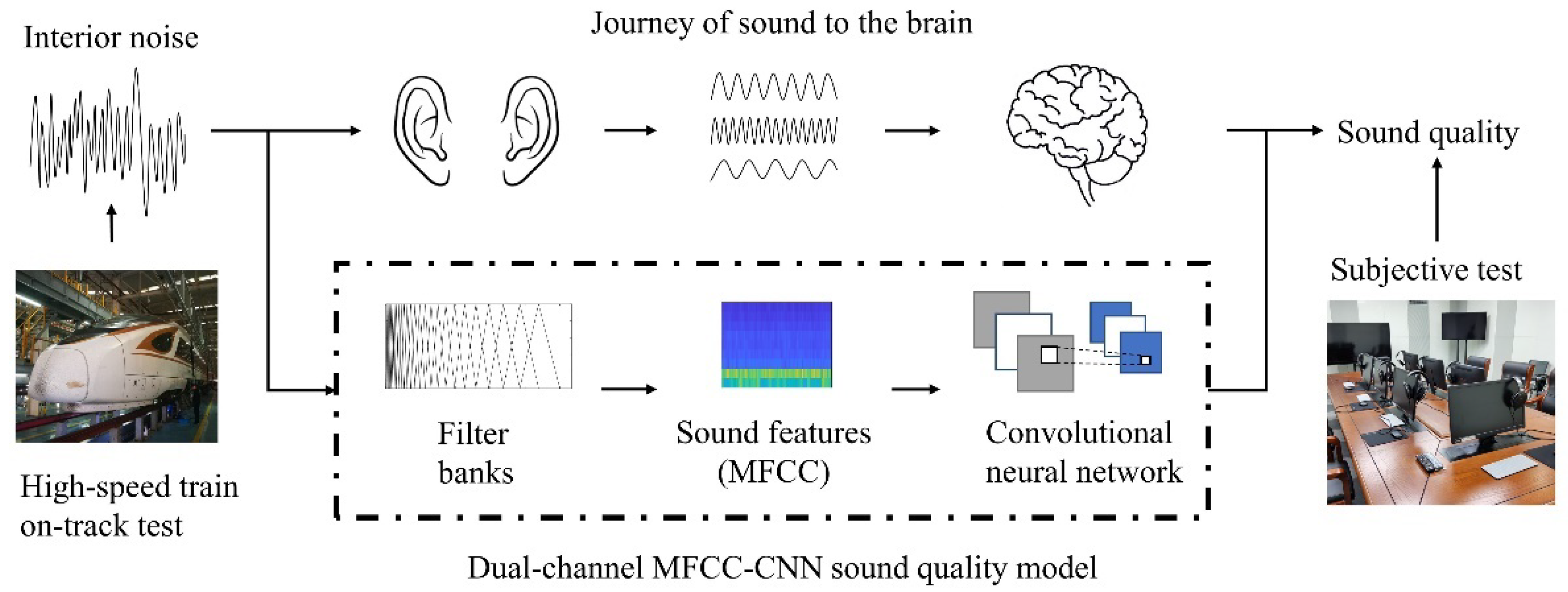
• The human auditory system works like a set of filters, so the model uses Mel-scale filter banks to simulate the system. The filter banks separate the input sound signal into multiple components and attenuate the components differently. Compared to the A-W SPL, the Mel-scale filter banks provide a better resolution at low frequencies and less resolution at high frequencies, which mimics the nonlinear human perception of sound.
• The model converts noise data into MFCC features, so both time domain and frequency domain information can be used simultaneously as input parameters for the CNN. At the same time, MFCCs help find out the key information in the noise sample, especially the low-frequency characteristics, thus improving the model accuracy.
• The CNN with multiple hidden layers is used to simulate the brain’s processing of sound signals. It is considered to be more powerful than traditional neural networks because of its high accuracy in speech recognition problems. Each layer of the CNN can be used to extract sound features.
• Two input channels are applied to simulate binaural hearing so that the different sound signals can be processed separately. The time and level differences of sound signals are important factors affecting sound quality.

The rest of this paper is organized as follows. The next section describes the collection of HST interior noise samples and how the subjective test is conducted. Section 3 explains the algorithm of the CNN and MFCC, and introduces a binaural MFCC-CNN sound quality model. Section 4 shows the results of the subjective test and the binaural MFCC-CNN model, together with a comparison with other models. The final section summarizes the conclusions of this paper.

2. Experimental Procedures

2.1. Noise Data Collection

The first part of the experiment was noise data collection. The collected noise samples were used to calculate the input parameters of the sound quality model. In addition, they were also used for the subjective test.

The noise measurement was carried out on a high-speed train (CR400BF) in China to collect noise samples. The train consisted of eight carriages. The carpet was laid on the floor; the seat covers were removed; and the doors remained closed. There were no passengers on the train. The train was running on a concrete track in an open field with a constant speed of 350 km/h. Twenty-two measuring points were arranged with reference to ISO 3381-2021 [22] in carriages 1, 3, 4, and 5. Areas with or without passenger seats were both considered. The noise in the driver’s cab was also recorded. The measuring points on the train are presented in Figure 2.

Noise data were recorded by an artificial head (HMS IV) from Head Acoustics. It was a binaural recording system with integrated electrostatic microphones. The frequency range was 3 Hz–20 kHz. The maximum SPL was 145 dB. The recording time was 30 s. The sampling rate was 48 kHz. Figure 3 demonstrates the experimental setup of the artificial head. Because there is only one artificial head, after a measurement point is recorded, the artificial head needs to be moved to a new measuring point.

2.2. Subjective Test

The subjective test was based on the subjective perception of sound by human beings, and the sound samples were evaluated according to the evaluation standard and rules. The subjective test can obtain the real judgement of noise and be used to verify the accuracy of the sound quality model.

There were 22 recorded noise samples from each measuring point. Each recorded noise sample was clipped to 5 s. The duration of each sample should not be too long; otherwise, the jury of the subjective test would be tired and make inaccurate judgments [19]. Besides, the noise samples should be clear without talking sound. The test length of each subject was approximately 15–25 min. The subjective evaluation process is shown in Figure 4. Figure 5 shows the Mel spectrogram of the binaural stimuli of some measuring points.

2.2.1. Subject Selection

The selection of subjects has an important influence on the results of subjective evaluation. Many factors such as the number of subjects, gender, and listening experience should be considered before the evaluation experiment. The number of subjects not only determines the workload of the experiment but also affects the reliability of the evaluation results. Generally, the more subjects, the better. Otto et al. [23] pointed out that 25–50 company employees as subjects can obtain accurate evaluation results. The subjects selected in this paper were 26 company employees (20 males and 6 females) from the China Railway Rolling Stock Corporation. Consent was obtained from all subjects involved in the study.

2.2.2. Jury Evaluation Method

Several popular jury evaluation methods are widely used in various applications. Each method has its strengths and weaknesses. It is important to choose an appropriate subjective evaluation method to obtain accurate subjective evaluation results. The ICBEN 5-point annoyance scale [24] was introduced to evaluate the annoyance level of HST noise subjectively. Subjects evaluate noise annoyance with five gradations. Each gradation was labeled with an appropriate adverb that allowed the subjects to judge the sound samples based on the subjects’ perceptions of sound combined with self-subjective sensations. Categorical scores were assigned to each gradation. The evaluation scores and their attributes are shown in

Table 1. Annoyance level and description.

Annoyance Level	1	2	3	4	5
Description	Not at all	Slightly	Moderately	Very	Extremely

.

2.2.3. Listening Environment and Test Delivery

The listening environment required by the subjective test has a great impact on the evaluation results, and a reasonable choice should be made according to the listening equipment used. The listening equipment used in this paper was the HD560 Sennheiser headphone. The listening experiment was conducted in an anechoic room to minimize the influences of ambient noise.

Instructions were given before the test to familiarize the subjects with both the sounds and the evaluation task. First, both the purpose of the evaluation and the evaluation method were explained. Then, subjects were trained to get used to the equipment with the sounds played back randomly. During the subjective evaluation, a form was provided to collect subjects’ responses. The samples were presented randomly to reduce the influence of presentation effects. All samples were randomly sorted three times to form three groups. Each subject heard a different play order and gave three scores for each sample.

3. Methods

3.1. Convolutional Neural Network (CNN)

The CNN is inspired by the way the brain processes vision. It is widely used in computer vision, natural language processing, and speech recognition. LeNet-5, a CNN that classifies digits, proposed by LeCun [25], is considered to be the foundation of modern CNNs. With the implementation of graphics processing units (GPUs), CNNs are greatly accelerated. More and more complex CNNs are proposed, such as Alexnet, VGGnet, and Resnet. A CNN is a feed-forward neural network and consists of an input layer, hidden layers, and an output layer. The hidden layers include layers that perform convolutions. A typical CNN architecture is illustrated in Figure 6.

3.1.1. Input Layer

The input layer receives single-channel (such as a grayscale image or single-channel noise signal) or multi-channel (such as a binaural voice signal or three-channel color image) data. The input layer shown in Figure 6 receives a three-channel RGB image. The input layer receives the input data and passes it to the convolutional layer.

3.1.2. Convolutional Layer

The convolutional layer is the core building block of a CNN. It contains many kernels (or filters). The main purpose of the convolutional layer is to use the kernel to extract certain features. Each kernel is convolved across the width and height of the input map from the previous layer, computing the dot product between the kernel and the input, and creating an activation map of that kernel.

Suppose the input is a tensor x with size H × W. The number of convolution kernels k is D, and the size of the kernel is m × n. The output of the convolutional layer can be expressed in the following equation:

$$y=f\left(k\ast x+b\right),$$

(1)

where y is the convolution output; b is the bias matrix; ∗ denotes the convolution operation; f is the activation function. The rectified linear unit (hence the name ReLU) activation function is often preferred to the other functions because it trains faster. It effectively removes negative values to increase the nonlinearity of the CNN. The ReLU activation function is calculated as follows:

$$g=max\left(0,z\right),$$

(2)

where g is the output; z is the input parameter.

The convolution output result has size (H – m + 1) × (W – n + 1) × D. Here is an example displaying the convolution operation in Figure 7.

The convolutional layer has a very strong feature learning ability. As the depth of the network increases, the extracted features tend to change gradually from low-level features to high-level features.

3.1.3. Pooling Layer

Another important part of the CNN is the pooling layer, which functions as non-linear down-sampling. It is common to insert a pooling layer after a convolutional layer. Generally speaking, the feature maps extracted by the convolutional layer have redundant information. The purpose of the pooling layer is to remove these redundant data and leave the most important data, thereby reducing the dimensions of data. The pooling layer plays an important part in preventing over-fitting. There are two types of pooling: max pooling and average pooling. Max pooling outputs the maximum value of the feature map, while average pooling takes the average value.

The operations of the max pooling and average pooling layer are shown in Figure 8. The filter size is 2 × 2. The pooling layer reduces the spatial size of the data, the number of parameters, and the amount of computation in the CNN.

3.1.4. Fully Connected Layer

Each neuron in the fully connected layer is connected to all neurons in the previous pooling layer or another layer. For an image classification task, the feature maps obtained after feature extraction from the input image are flattened into one vector, which becomes the input of the fully connected layer. The output of the fully connected layer can be expressed as:

$$y=f\left(wx+b\right),$$

(3)

where y is the output of the fully connected layer; x is the input of the fully connected layer; w is the weight matrix; b is the bias matrix; and f denotes the activation function.

3.1.5. Output Layer

In the classification task, the output layer usually uses the softmax activation function as a classifier. The softmax function is expressed as:

$$\sigma {\left(Z\right)}_i=\frac{e^{Z_i}}{{\sum }_{j=1}^K{e}^{Z_j}} ,$$

(4)

where Z is the input vector of K real numbers; Z = (Z₁, Z₂ …… Z_K) and i = 1, 2, ……, K.

The softmax function takes vector Z as input and normalizes it into a probability distribution consisting of K probabilities that add up to 1.

3.2. Mel-Scale Frequency Cepstral Coefficients (MFCC)

The MFCC is a feature extracted from sound signals and widely used in automatic speech recognition (ASR). The human auditory system works like a set of filters. It responds differently at different frequencies. Humans are much more sensitive to small changes in low frequencies than they are at high frequencies. The Mel scale filter banks simulate the human auditory system by being more discriminative at lower frequencies and less discriminative at higher frequencies. The Mel (m) scale can be converted from Hertz (f) using the following equation:

$$m=2595lo{g}_{10}\left(1+\frac{f}{700}\right).$$

(5)

Each filter in the filter banks is a triangular filter. It has a response of 1 at the center frequency and decreases linearly to 0 when it reaches the center frequencies of the two adjacent filters. The filter banks in this paper’s sound quality model contain 26 filter banks. It starts at 0 Hz and ends at 20,000 Hz, as shown in Figure 9.

The filter bank coefficients are obtained after applying filter banks to the power spectrum of the sound signal. Then, take the log of each of the 26 coefficients. The discrete cosine transform (DCT) is applied to decorrelate the 26 log coefficients and to give 26 Mel frequency cepstral coefficients. Figure 10 shows the steps involved in MFCC feature extraction.

3.3. Binaural MFCC-CNN Sound Quality Model

The proposed binaural MFCC-CNN sound quality model was built on MATLAB to study the relationship between the subjective evaluation and HST interior noise. The architecture is displayed in Figure 11. The MFCC of the sound signal was used as input to the model.

In order to train a CNN model better, original sound data from each measuring point were divided into multiple one-second segments to generate more training data. Each recorded interior noise signal was split into 30 noise samples, and a total of 660 noise samples are obtained. HST interior noise can be regarded as stationary signals at the same speed, so it was reasonable to assign the same subjective evaluation score to the noise samples from the same measuring points [19].

The signal was framed into 25 ms each frame with an overlap length of 15 ms, so there were 98 frames in each sample. Twenty-six filter banks were applied to each frame, so 26 MFCC coefficients were extracted. Thus, the input data size was 98 × 26 for each input channel.

The size of convolutional layers C1–C4 was 3 × 3 with a stride of 1 and no padding. The number of filters in C1 and C3 was 16. The number of filters in C2 and C4 was 32. The ReLU activation function was applied after each convolutional layer. The method in pooling layers P1–P4 was max pooling. The size was 3 × 3 with a stride of 2 and no padding. The number of neurons in Fc1 and Fc2 was 50. An additional layer was implemented after Fc1 and Fc2 to simulate the summation of the intensity of sound. It adds inputs from the previous layer. The size of Fc3 was set to 5 for classification because there are 5 annoyance levels. The output layer contains the softmax layer and classification layer.

To validate the binaural MFCC-CNN model, 80% of noise samples in each scale were put into the training data set, while the remaining 20% of noise samples were used to test the performance of the training model. Some training parameters need to be specified before training. The initial learning rate was 0.005, and it dropped to its half every 50 epochs. The maximum epoch was 1000 epochs. The mini-batch size was 32. The training used a single Nvidia RTX 3090 graphic card.

4. Results and Discussions

4.1. Subjective Evaluation Results and Data Check

The Kendall concordance coefficient was employed to check the consistency of the standard of a single subject across all participants. The Kendall concordance coefficient ranges from 0 (no agreement) to 1 (complete agreement). Suppose that there are total n sound samples and m subjects, where sample i is given the rank $r_{i,j}$ by subject number j. Then, the total rank $R_i$ given to object i is:

$$R_i={\displaystyle \sum }_{j=1}^m{r}_{i,j} .$$

(6)

The mean value $\overline{R}$ of these total ranks is:

$$\overline{R}=\frac{1}{n}{\displaystyle \sum }_{i=1}^n{R}_i .$$

(7)

The Kendall concordance coefficient W is calculated as follows:

$$W=\frac{12{\sum }_{i=1}^n{(R_i-\overline{R})}^2}{m^2\left(n^3-n\right)}.$$

(8)

The Kendall concordance coefficient of each subject is shown in Figure 12.

The maximum coefficient was 0.94 (subject number 14), and the minimum coefficient was 0.43 (subject number 22). The criterion for screening the results of the subjective evaluation was 0.6. Thus, the subjective responses from three subjects were eliminated. The Kendall concordance coefficient across all subjects was 0.86. This meant that a similar standard was applied to the evaluation of the 23 subjects.

Generally, subjects’ evaluation of the same sample follows the law of normal distribution. The Lilliefors test was conducted to check whether the response data belong to the family of normal distributions. Figure 13a shows the subjects’ responses’ distribution of noise of measuring point 11. The Lilliefors test of each measuring point was conducted in MATLAB 2020a, and the results were shown in Figure 13b. The returned value of h = 0 indicates that the Lilliefors test does not reject the null hypothesis at the 1% significance level, so the subjective results of all the measuring points followed the law of normal distribution.

The mean values and standard deviation of subjective responses of each noise sample are shown in Figure 14. The highest evaluation appears at point number 22 (windshield area in carriage 5), and the lowest evaluation appears at point number 8 (carriage 3). The standard deviation is relatively small which shows that the subjective evaluations were clustered closely, and subjects followed the same standard.

4.2. Training Results of the Binaural MFCC-CNN Model

The training progress of the binaural MFCC-CNN model is shown in Figure 15. After training, the accuracy of the proposed model was evaluated by testing the data set. The accuracy of the testing data set reached 96.2%, indicating that the proposed model was feasible for sound quality evaluation and that the CNN method was appropriate. Figure 16 displays the accuracy matrix of the testing data set to measure the effectiveness of the proposed model. The diagonal elements represent the number of samples for which the predicted evaluation is equal to the actual evaluation. The testing data set contained 132 noise samples, and the model made a total of 132 evaluations.

From the subjective test results in Figure 14, the evaluated noise samples were categorized into four scales. If the mean value was smaller than 1.5, the measuring points were labeled as ‘Not at all’. For measuring points with a mean value between 1.5 and 2.5, they were rated as ‘Slightly’. Then, the points with a mean value between 2.5 and 3.5 were rated as ‘Moderately’. The points were rated as ‘Very’ if the mean value was between 3.5 and 4.5. Because the highest mean value was 4.27 at point 22, no points were rated as ‘Extremely’.

The binaural MFCC-CNN model made an accurate assessment. It predicted ‘Not at all’ 31 times, ‘Slightly’ 36 times, ‘Moderately’ 34 times, and ‘Very’ 31 times. The model made 127 accurate evaluations and missed 5, so the testing accuracy was 127/132 (96.2%). One ‘Not at all’ was wrongly evaluated as ‘Slightly’, and two ‘Slightly’ were wrongly evaluated as ‘Not at all’. To improve the accuracy, it is important to increase the number of samples of ‘Not at all’ and ‘Slightly’ to train the model better.

4.3. Performance Comparison with Other Models

4.3.1. Shallow Neural Network Model

To compare the performance of the binaural MFCC-CNN model, a shallow neural network sound quality model was built and is shown in Figure 17. Seven commonly used parameters (A-W SPL, loudness, sharpness, roughness, fluctuation strength, articulation index, tonality) were applied as inputs of the model; the output was annoyance level. The input layer, hidden layer, and output layer contain seven nodes, four nodes, and one node, respectively. The number of noise samples in the shallow neural network model is the same as that in the binaural MFCC-CNN sound quality model. The same subjective results were used to compare the performance of this shallow neural network model and the binaural MFCC-CNN model. Figure 18 presents the evaluation result of the shallow neural network model. Although the predicted value of each measuring point is very close to the actual value, the model accuracy (91.1%) is lower than the binaural MFCC-CNN model. One possible reason is that the input parameters in the shallow model do not consider the influence of the time-varying characteristics of the sound samples, so the binaural MFCC-CNN model performs better in the evaluation of sound quality.

4.3.2. The Influence of Binaural Hearing and MFCC

Humans receive sound with two ears, but in many studies, the sound quality models were constructed with only one input channel. The single-input models did not consider the difference in sound between the two ears. Therefore, a monaural MFCC-CNN model was established to investigate further whether considering binaural hearing would help the model perform better in the sound quality evaluation. At the same time, a model that used time series data as input was also created to verify whether MFCC features helped to improve the evaluation accuracy. The structure of the two models is shown in Figure 19.

The training progress of the two models is shown in Figure 20. The testing accuracy of the monaural MFCC-CNN model reached 91.7%, and the binaural time series CNN model had a lower testing accuracy (87.1%). The accuracy of both models was lower than the binaural MFCC-CNN model.

Comparing the monaural and binaural models, it is clear that the evaluation is more accurate with extra input. On the one hand, an extra input channel provides more noise data; thus, more sound features are provided. On the other hand, the difference between the input data has a significant impact on the accuracy of the model, and such a difference is also an important factor for the subjective evaluation of sound quality. Meanwhile, although the time series model uses a binaural input, the accuracy (87.1%) of the model is even lower than that of the shallow neural network model. Generally, the model can have all the original information from the input time series data. However, the amount of time-domain data is relatively large and full of unnecessary information, and it is difficult for the model to find the key feature that affects the subjective evaluation. For this reason, the application of MFCC features not only helps reduce the input data dimensions but also provides frequency domain information that facilitates the distinction of various noise samples and improves the accuracy of the model.

To investigate the prediction distribution further, the confusion matrix of testing accuracy of each model is shown in Figure 21. In Figure 21a, the highest accuracy (97.2%) appears at ‘Moderately’, while the lowest accuracy (86.7%) appears at ‘Not at all’. Compared with the binaural MFCC-CNN model, the monaural MFCC-CNN model is less accurate in the assessment of ‘Not at all’ and ‘Slightly’. Two ‘Not at all’ responses are wrongly evaluated as ‘Moderately’, and three ‘Slightly’ responses are wrongly evaluated as ‘Moderately’. It appears that the monaural model is more willing to evaluate the sample as ‘Moderately’. Perhaps the time and the level difference between the two ears are crucial factors affecting the subjective evaluation at a low annoyance level. However, the monaural MFCC-CNN model could not take such differences into account, which causes lower accuracy. As can be seen from Figure 21b, the binaural time series CNN model has the highest accuracy (93.3%) in ‘Not at all’ and the lowest accuracy (83.3%) in ‘Very’. The accuracy decreases with the increase in annoyance level.

Comparing the three CNN models shows that the binaural MFCC-CNN model has better accuracy for each annoyance level. The monaural MFCC-CNN model has poor accuracy for samples in ‘Not at all’ and ‘Slightly’, indicating that an extra input has an important influence on the low annoyance level samples. Meanwhile, the binaural time series CNN model has the lowest accuracy among all models in the scale ‘Very’, suggesting that MFCC features can improve the accuracy of samples by capturing the characteristics of noise with a high annoyance level.

5. Conclusions

In this paper, a binaural sound quality model for HSTs was developed using CNN techniques. In order to obtain sufficient training samples, a HST on-track test was carried out to collect the interior noise data. To train the sound quality model and verify its accuracy, the collected noise was subjectively evaluated using a five-scale semantic differential method. The conclusions are summarized as follows:

• The binaural MFCC-CNN sound quality model has a similar architecture to the hearing system. It better represents the nonlinearity of human hearing and makes the model highly accurate. The model achieved an accuracy of 96.2%. Thus, the proposed model was feasible for the HST sound quality evaluation, and the CNN method was appropriate.
• The sound signals were converted into MFCC features as input parameters for the CNN, so both time domain and frequency domain information can be considered simultaneously. The proposed model considered the influence of the time-varying characteristics of the sound, which led to better performance than the traditional neural network model.
• Two input channels were applied to simulate binaural hearing. The time and the level difference between the two ears were important factors affecting the HST subjective evaluation, and such differences also affected the accuracy of the sound quality model, especially at a low annoyance level. Hence, the monaural MFCC-CNN sound quality model had lower accuracy than the binaural model.
• The MFCC features extracted from the sound signal helped capture the main characteristics of HST noise at high annoyance levels and reduced the input data dimensions. It provided frequency domain information that facilitates the distinction of various noise samples, so the proposed model outperformed the times series sound quality model.

Overall, the results show that the proposed model can be used to evaluate and optimize the HST interior sound quality, reducing man labor and material resources. To improve the proposed model, it will be important that future research investigates the sound quality of HSTs under different operating conditions (for example, different speeds) as well as the impact of transient noise.

References

1. Münzel, T.; Sørensen, M.; Daiber, A. Transportation noise pollution and cardiovascular disease. Nat. Rev. Cardiol. 2021, 18, 619–636. [Google Scholar] [CrossRef] [PubMed]
2. Peng, Y.; Fan, C.; Hu, L.; Peng, S.; Xie, P.; Wu, F.; Yi, S. Tunnel driving occupational environment and hearing loss in train drivers in China. Occup. Environ. Med. 2019, 76, 97–104. [Google Scholar] [CrossRef] [PubMed]
3. Qian, K.; Hou, Z.; Sun, Q.; Gao, Y.; Sun, D.; Liu, R. Evaluation and optimization of sound quality in high-speed trains. Appl. Acoust. 2021, 174, 107830. [Google Scholar] [CrossRef]
4. Standard ISO 532-1:2017; Acoustics—Methods for Calculating Loudness—Part 1: Zwicker Method. International Organization for Standardization: Geneva, Switzerland, 2017.
5. Standard ISO 532-2:2017; Acoustics—Methods for Calculating Loudness—Part 2: Moore-Glasberg Method. International Organization for Standardization: Geneva, Switzerland, 2017.
6. Luo, L.; Zheng, X.; Hao, Z.-Y.; Dai, W.-Q.; Yang, W.-Y. Sound quality evaluation of high-speed train interior noise by adaptive Moore loudness algorithm. J. Zhejiang Univ. A 2017, 18, 690–703. [Google Scholar] [CrossRef]
7. Liu, Z.; Sun, Z.; Liu, S. Study on the Sound Quality Objective Evaluation of High Speed Train’s Door Closing Sound. In Proceedings of the 2015 International Forum on Energy, Environment Science and Materials, Shenzhen, China, 25–26 September 2015. [Google Scholar] [CrossRef] [Green Version]
8. Chen, X.; Lin, J.; Jin, H.; Huang, Y.; Liu, Z. The psychoacoustics annoyance research based on EEG rhythms for passengers in high-speed railway. Appl. Acoust. 2021, 171, 107575. [Google Scholar] [CrossRef]
9. Park, B.; Jeon, J.-Y.; Choi, S.; Park, J. Short-term noise annoyance assessment in passenger compartments of high-speed trains under sudden variation. Appl. Acoust. 2015, 97, 46–53. [Google Scholar] [CrossRef]
10. Hong, J.; Cha, Y.; Jeon, J.Y. Noise in the passenger cars of high-speed trains. J. Acoust. Soc. Am. 2015, 138, 3513–3521. [Google Scholar] [CrossRef] [PubMed]
11. Yoon, K.; Gwak, D.Y.; Chun, C.; Seong, Y.; Hong, J.; Lee, S. Analysis of frequency dependence on short-term annoyance of conventional railway noise using sound quality metrics in a laboratory context. Appl. Acoust. 2018, 138, 121–132. [Google Scholar] [CrossRef]
12. Meng, F.; Yang, L. Sound Quality Evaluation on Interior Noise in High-speed Trains. In Proceedings of the 40th Annual German Congress on Acoustics, Oldenburg, Germany, 10–13 March 2014. [Google Scholar]
13. Chen, P.; Xu, L.; Tang, Q.; Shang, L.; Liu, W. Research on prediction model of tractor sound quality based on genetic algorithm. Appl. Acoust. 2022, 185, 108411. [Google Scholar] [CrossRef]
14. Xing, Y.F.; Wang, Y.S.; Shi, L.; Guo, H.; Chen, H. Sound quality recognition using optimal wavelet-packet transform and artificial neural network methods. Mech. Syst. Signal Process. 2016, 66–67, 875–892. [Google Scholar] [CrossRef]
15. Liu, H.; Zhang, J.; Guo, P.; Bi, F.; Yu, H.; Ni, G. Sound quality prediction for engine-radiated noise. Mech. Syst. Signal Process. 2015, 56–57, 277–287. [Google Scholar] [CrossRef]
16. Lee, H.; Lee, J. Neural network prediction of sound quality via domain Knowledge-Based data augmentation and Bayesian approach with small data sets. Mech. Syst. Signal Process. 2021, 157, 107713. [Google Scholar] [CrossRef]
17. Huang, H.B.; Wu, J.H.; Huang, X.R.; Yang, M.L.; Ding, W.P. The development of a deep neural network and its application to evaluating the interior sound quality of pure electric vehicles. Mech. Syst. Signal Process. 2019, 120, 98–116. [Google Scholar] [CrossRef]
18. Liang, K.; Zhao, H. Automatic evaluation of internal combustion engine noise based on an auditory model. Shock Vib. 2019, 2019, 2898219. [Google Scholar] [CrossRef] [Green Version]
19. Huang, X.; Huang, H.; Wu, J.; Yang, M.; Ding, W. Sound quality prediction and improving of vehicle interior noise based on deep convolutional neural networks. Expert Syst. Appl. 2020, 160, 113657. [Google Scholar] [CrossRef]
20. Zhao, B.; Wu, C.J. Sound quality evaluation of electronic expansion valve using Gaussian restricted Boltzmann machines based DBN. Appl. Acoust. 2020, 170, 107493. [Google Scholar] [CrossRef]
21. Monaragala, R.M. Knitted structures for sound absorption. In Advances in Knitting Technology; Woodhead Publishing: Sawston, UK, 2011; pp. 262–286. [Google Scholar] [CrossRef]
22. Standard ISO 3381:2021; Railway applications—Acoustics—Noise Measurement Inside Railbound Vehicles. International Organization for Standardization: Geneva, Switzerland, 2021.
23. Otto, N.; Amman, S.; Eaton, C.; Lake, S. Guidelines for jury evaluations of automotive sounds. SAE Tech. Pap. 1999, 108, 3015–3034. [Google Scholar] [CrossRef] [Green Version]
24. Gjestland, T. Standardized general–purpose noise reaction questions. In Proceedings of the 12th ICBEN Congress, Zurich, Switzerland, 18–22 June 2017. [Google Scholar]
25. Lecun, Y.; Bottou, L.; Bengio, Y.; Haffner, P. Gradient-based learning applied to document recognition. Proc. IEEE Inst. Electr. Electron. Eng. 1998, 86, 2278–2324. [Google Scholar] [CrossRef]
Figure 1. The basic structure of the binaural MFCC-CNN sound quality model.
Applsci 12 12151 g001
Figure 2. Twenty-two measuring points (Red numbers) in carriages 1, 3, 4, 5.
Applsci 12 12151 g002
Figure 3. Experimental setup of the artificial head.
Applsci 12 12151 g003
Figure 4. Subjective evaluation process.
Applsci 12 12151 g004
Figure 5. Mel spectrogram: (a) Measuring point 1 Left; (b) Measuring point 1 Right; (c) Measuring point 7 Left; (d) Measuring point 7 Right; (e) Measuring point 13 Left; (f) Measuring point 13 Right.
Applsci 12 12151 g005aApplsci 12 12151 g005b
Figure 6. Typical CNN architecture.
Applsci 12 12151 g006
Figure 7. Convolution operation.
Applsci 12 12151 g007
Figure 8. Pooling operation.
Applsci 12 12151 g008
Figure 9. Mel-scale filter banks.
Applsci 12 12151 g009
Figure 10. MFCC feature extraction process.
Applsci 12 12151 g010
Figure 11. Binaural MFCC-CNN sound quality model.
Applsci 12 12151 g011
Figure 12. Kendall concordance coefficient of each subject.
Applsci 12 12151 g012
Figure 13. Normality test: (a) Subjective responses’ distribution of point 11; (b) Hypothesis test results of each measuring point.
Applsci 12 12151 g013
Figure 14. Subjective evaluation of each measuring point.
Applsci 12 12151 g014
Figure 15. Training progress of the binaural MFCC-CNN model: (a) Training accuracy; (b) Training loss.
Applsci 12 12151 g015
Figure 16. Confusion matrix of testing data set of the binaural MFCC-CNN model.
Applsci 12 12151 g016
Figure 17. Shallow neural network sound quality model.
Applsci 12 12151 g017
Figure 18. Evaluation performance of the shallow neural network model.
Applsci 12 12151 g018
Figure 19. Different sound quality prediction models for comparison: (a) Monaural MFCC-CNN model; (b) Binaural time series CNN model.
Applsci 12 12151 g019
Figure 20. The training progress of different sound quality models: (a) Training accuracy and (b) Training loss of the monaural MFCC-CNN model; (c) Training accuracy and (d) Training loss of the binaural time series CNN model.
Applsci 12 12151 g020
Figure 21. Confusion matrix of (a) The monaural MFCC-CNN model; (b) The binaural time series CNN model.
Applsci 12 12151 g021