mmSight: A Robust Millimeter-Wave Near-Field SAR Imaging Algorithm

Abstract

Millimeter-wave SAR (Synthetic Aperture Radar) imaging is widely studied as a common means of RF (Radio Frequency) imaging, but there are problems of the ghost image in Sparsely-Sampled cases and the projection of multiple targets at different distances. Therefore, a robust imaging algorithm based on the Analytic Fourier Transform is proposed, which is named mmSight. First, the original data are windowed with Blackman window to take multiple distance planes into account; then, the Analytic Fourier Transform that can effectively suppress the ghost image under Sparsely-Sampled is used for imaging; finally, the results are filtered using a Mean Filter to remove spatial noise. The experimental results show that the proposed imaging algorithm in this paper, relative to other algorithms, can image common Fully-Sampled single target, hidden target, and multiple targets at the same distance, and solve the ghost image problem of single target in the case of Sparsely-Sampled, as well as the projection problem of multiple targets at different distances; the Image Entropy of the mmSight is 4.6157 and is on average 0.3372 lower than that of other algorithms. Compared with other algorithms, the sidelobe and noise of the Point Spread Function are suppressed, so the quality of the image obtained from imaging is better than that of other algorithms.

1. Introduction

With the development of information technology, an increasing number of intelligent applications have started to appear. Within this trend, a large number of intelligent applications build intelligent systems, such as the “smart city” mentioned in the literature [1], which can maximize the use of limited resources to manage the city with high quality. However, as an intelligent system, it needs enough information to make reasonable judgments, but information is diverse; sounds, pictures, and smells are all information, and to obtain them is just like the human sensing process. Thus, various sensors are designed to implement a certain function of human sensing; for example, a camera is like an eye to get visual information. However, intelligent systems are not limited to this; they can see much more. While cameras are affected by lighting conditions and do not have the ability to penetrate, there are technologies that are not affected by lighting and can penetrate the surface to see the essence, such as X-rays, which can see the state of a patient’s internal organs. The literature [2,3] illustrates the value that this imaging technique brings to intelligent systems, where capturing the information, aided by AI techniques, allows for a quick and accurate determination of the disease. Its non-contact characteristic is more valuable in the background of COVID-19 ravaging the world. However, X-rays are expensive and radioactive, limiting the environment in which they can be applied. Therefore, intelligent systems need cheaper and safer RF imaging technology to meet a wider range of application environments.

As an advanced application in the field of wireless sensing, RF imaging has received a lot of attention, and the introduction of “wireless vision” in [4] indicates that RF imaging has become a new research hotspot in the field of wireless sensing, which requires finer sensing granularity than most sensing fields. However, the development of RF imaging has not been smooth and has long been constrained by insufficient imaging resolution and aperture. Currently, mmWave-based SAR imaging technology has the advantages of greater imaging bandwidth and stronger imaging aperture expansion, and has become one of the enabling technologies for RF imaging to meet fine-grained sensing needs in near-field conditions. There have been many studies based on millimeter-wave SAR imaging technology. Various millimeter-wave SAR near-field imaging systems developed in the literature [5,6,7,8,9,10] were successfully used for security screening. The authors of [11] developed a simple 77 GHz millimeter wave SAR near-field imaging system using a commercial millimeter-wave radar and rails. In the literature [12], a low-cost 24 GHz millimeter-wave SAR near-field imaging system was implemented using Hilbert transform to compensate for the real signal. Although the available studies have reduced the system cost and improved the imaging quality, there are still some challenges.

SAR uses the time-for-space tactics, which makes its data acquisition time long. Sometimes, in order to quickly verify the imaging method, data have to be acquired under Sparsely-Sampled conditions. This generates ghost image and is not conducive to the analysis of imaging results, so it is necessary to suppress ghost image under Sparsely-Sampled conditions. The authors of [13] solve the Sparsely-Sampled ghost image problem under MIMO (Multiple Input Multiple Output) conditions, but does not address the problem under SISO (Single Input Single Output) conditions. The work in this paper still addresses the case of uniform sampling. In addition to the uniform sampling technique, the authors of [14] use a non-uniform hybrid sampling technique to construct a SAR imaging system that achieves high-resolution imaging. In addition, the work in this paper is performed for the Analytic Fourier Transform algorithm, while in [15] it is performed for the Frequency Scaling algorithm (FSA), and the FSA is improved to eliminate the impact of the aliasing effect. In addition, in order to obtain as much information as possible, it is often necessary to project multiple targets that are in neighboring different distance planes onto one distance plane, which is not available in conventional imaging algorithms and requires more processing steps, so a one-step projection method can greatly reduce the workload. The problem of projecting multiple targets at different distances planes to the same distance plane was solved in the literature [16,17] using the Maximum Projection method, but it requires a combination of multiple results to achieve this, which cannot be achieved in one step.

In summary, there are still many challenges in the field of millimeter-wave SAR imaging, especially the ghost image problem of SISO Sparsely-Sampled and the projection problem of multiple targets at different distances. Therefore, this paper addresses these challenges and does related research, and the contributions made are as follows.

• A simple millimeter-wave near-field SAR imaging system is developed with an easy-to-build “T” structure for the rail part, and the complexity of the radar part is reduced by using the SISO, monostatic approach.
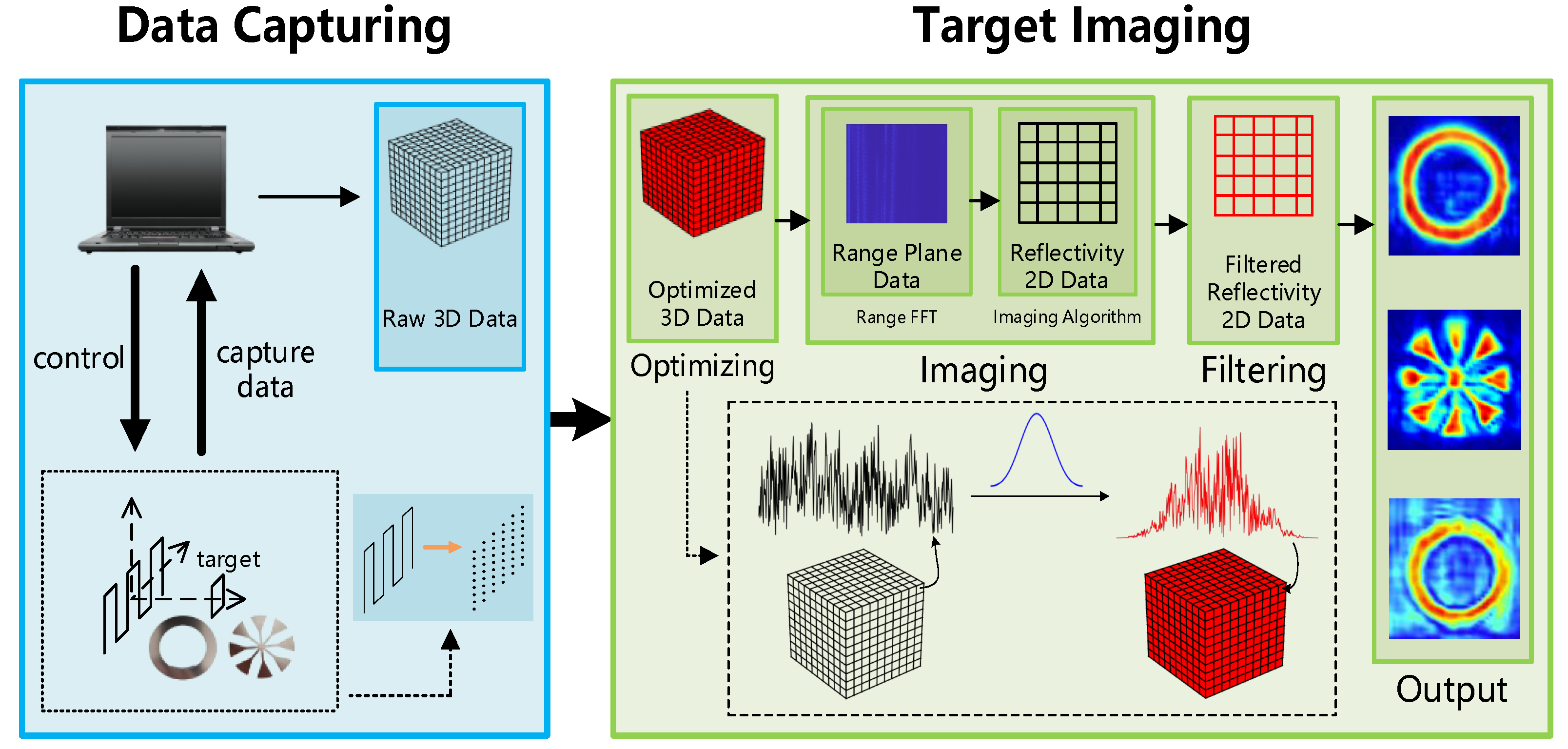
• A robust millimeter-wave SAR imaging method is proposed, including three parts: windowing, imaging, and noise reduction. The Blackman Window used aims at the projection problem of multiple targets at different distances, the Analytic Fourier Transform imaging algorithm used aims at ghost image under SISO Sparsely-Sampled, and the Mean Filter used aims at spatial noise.
• We have conducted a large number of imaging experiments, and the results show that the mmSight can image a single target with Fully-Sampled, a hidden target, and multiple targets at the same distance, in addition to solving the ghost image problem under SISO Sparsely-Sampled conditions and the projection problem of multiple targets at different distances, which indicates that the mmSight enhances the robustness of the imaging system.

This paper consists of five sections. Section 2 introduces the work related to millimeter wave imaging; Section 3 details the proposed imaging method, which mainly contains two parts: data acquisition and target imaging; Section 4 shows the experimental platform, experimental results, and also evaluates the experimental results; Section 5 concludes the paper.

2. Related Work

Current millimeter-wave near-field imaging is based on a variety of technical solutions, and the mainstream technology is dominated by various forms of SAR. In addition, there are still some non-SAR solutions. In this section, we introduce the related work from these two types of imaging technologies and describe the related research progress around the world.

2.1. Non-SAR Imaging of mmWave

Each non-SAR approach has its own characteristic. The literature [18] used WiFi for through-wall imaging to achieve the marking of key parts of the human body. The literature [4] used commercial 60 GHz WiFi with self-designed micro-antenna arrays to achieve low-resolution human pose imaging for small devices. Point cloud imaging can satisfy real-time, but the resolution is often unsatisfactory, so the deep learning network designed in the literature [19] enhances the point cloud data and obtains an imaging resolution close to SAR. In addition, the authors of [20] combined wireless signals with image signals to achieve a wireless-signal based human contour generation task. Through the above work, it can be seen that the raw resolution of non-SAR imaging is generally not high, and other auxiliary means are required to enhance the imaging resolution. Therefore, SAR is still one of the key technologies in the field of imaging.

2.2. SAR Imaging of mmWave

The SAR imaging approach, which refers to the relative motion between radar and target, then uses signal processing techniques to achieve imaging. In the simplest SAR imaging, the target does not move, and the radar moves to produce a virtual array with a large aperture; for example, [11] used a rail system to drive the radar motion while the 2D (Two-Dimensional) target was fixed on a stand, and eventually, the collected data was processed to obtain the final 2D imaging results. The literature [21,22], on the other hand, used a more powerful radar with a longer rail to achieve imaging of a 3D (Three-Dimensional) target. In addition, [23] extends the range of motion of the radar from two-dimension to three-dimension, and as a result, different virtual arrays are obtained, deriving imaging algorithms adapted to the new arrays. There is also CSAR (Circular Synthetic Aperture Radar), the radar of which rotates along a cylindrical trajectory, which was used in the literature [24,25,26]. Compared to the common SAR, ISAR (Inverse Synthetic Aperture Radar) allows the target to move as well. The authors of [27] let the target knife rotate while combining the traditional SAR, derived the imaging algorithm in this scenario, and obtained different imaging results at different moments. The authors of [28] investigated imaging under irregular curved motion trajectories. Our work’s advantages are shown in

Table 1. Compared to some related works.

Source	Antenna Mode	Eliminate Ghost Image	Different-Distances Projection
This Work	SISO	Yes	Yes
[13]	MIMO	Yes	No
[16]	SISO	No	Yes
[12]	SISO	No	No

.

In this paper, the SAR approach is still used for imaging in order to achieve the goal of high resolution and make the algorithm simple, and instead of using the MIMO approach as in the literature [13], the SISO approach is chosen for the simplicity of implementation. The problem of ghost image is also solved under SISO using the relevant algorithm. In addition, there are more studies on MIMO imaging; for example, the authors of [29] explored the imaging problem of special cross-shaped MIMO arrays and designed a corresponding imaging algorithm to accomplish target reconstruction. However, there are fewer studies on SISO.

3. System Design

This section describes the design of the system, firstly introducing the overall structure of the system, and then detailing the two parts of data acquisition and target imaging, respectively.

3.1. System Overview

The workflow of the whole imaging system is shown in Figure 1. The workflow is divided into two stages, the first stage is Data Capturing, and the second stage is Target Imaging. In the Data Capturing stage, a computer-controlled rail system is used to drive the radar movement to build a virtual array, complete the data acquisition of the target, and finally get the original 3D data (the three dimensions are vertical orientation, horizontal orientation, and time), and use this data as the input of the next stage. In the Target Imaging stage, the original 3D data are first optimized by adding Blackman window for each IF (Intermediate Frequency) signal in the original 3D data, and the optimized 3D data are finally obtained. Then the optimized 3D data are used as the input of the imaging algorithm, and the reflectivity data (which can already be used as the imaging result) is obtained after the algorithm processing. Finally, two-dimensional mean filtering is performed on the reflectivity data to remove spatial noise and obtain the optimized reflectivity data, and finally the imaging result is produced.

3.2. Data Capturing

In the system constructed in this paper, the rail part is responsible for the radar motion. The radar starts from the lower left corner of the scanning plane (primed coordinates) and moves along the zigzag. During the motion, the data are collected in two directions, vertical and horizontal, at equal interval, as shown at the top of Figure 2. The motion of this system is in discrete motion mode, with the radar acquiring data when stopped and the radar pausing to acquire data when in motion. After the motion is completed, a virtual aperture array equivalent to the real aperture array can be obtained, as shown at the bottom left of Figure 2, where, $D_x$ denotes the length of the horizontal aperture, $D_y$ denotes the length of the vertical aperture, $d_x$ denotes the spatial sampling interval in the horizontal direction, and $d_y$ denotes the spatial sampling interval in the vertical direction.

3.2.1. FMCW Signal Model

The radar part is responsible for signal transceiving. The chirp signals transmitted by the FMCW (Frequency-Modulated Continuous Wave) radar used in this paper are:

$$m(t)=A\cos \left[2\pi (f_{0}t+K{t}^2/2)+\phi \right]$$

(1)

The transmitted signal is reflected from the target after a round-trip delay $\tau$, at which point the received signal is:

$$b(t)=A\cos \left[2\pi (f_0(t-\tau )+K{(t-\tau )}^2/2)+\phi \right]$$

(2)

Then, within the radar, the transmitted and received signals are mixed and low-pass filtered to produce an IF signal, which can be expressed as:

$$r_I(t)=A\cos \left[2\pi (f_{b}t+f_0\tau -K{\tau }^2/2)\right]$$

(3)

where, $f_b=K\tau$ is the frequency of the IF signal, and the last term $K{\tau }^2/2$, as the residual video phase, is generally neglected due to its relatively small value in near-field conditions. In addition to transmitting one way I (In-phase) signal, the radar also transmits one way Q (Quadrature) signal that is orthogonal to the I signal. Thus, the obtained IF IQ (In-phase and Quadrature) signal can be expressed as:

$$r(t)=r_I(t)+j{r}_Q(t)=A{e}^{j2\pi (f_{b}t+f_0\tau )}.$$

(4)

3.2.2. Original Data

At each spatial sampling point, the radar antenna operates in SISO mode, transmitting and receiving only one chirp signal. Besides, due to the close distance between the transceiver, the Equivalent Phase Center (EPC) principle can be used to approximate the operation of a monostatic antenna by using the midpoint of the transceiver instead of the transceiver, as shown in the lower right side of Figure 2. In the figure, TX (transmit) denotes the transmitting antenna of SISO, RX (receive) denotes the receiving antenna of SISO, and the point between them is the equivalent phase center point, and the location of the point is replaced by a virtual monostatic antenna; R denotes the distance between the antenna array plane and the target plane, and the total distance of the signal from transmitting to receiving is 2R. After the IF signal at each sampling point is collected, the radar cube data are obtained, as shown in Figure 3.

The 3D data are obtained, and after dealing with distance-FFT (Fast Fourier Transform) and pulse compression, the relevant data in the target plane is retained and the data in other planes are filtered out to obtain the required target plane information [11]:

$$s(x^{\prime },y^{\prime })={\displaystyle {\int }_0^{T}r(x^{\prime },y^{\prime },t)}{e}^{-j2\pi K{\tau }_{0}t}dt$$

(5)

where, $K{\tau }_0$ denotes the frequency of the IF signal corresponding to the target plane (distance $z_0$).

3.3. Target Imaging

The target imaging stage is divided into three steps, namely windowing, imaging, and filtering. The algorithm used for windowing is the Blackman window, the algorithm used for imaging is the Analytic Fourier Transform, and the algorithm used for filtering is the two-dimensional Mean Filter, and the results obtained in each step are shown in Figure 1.

3.3.1. Windowing with Blackman

Windowing is to optimize each chirp of the original 3D data using a Blackman window, and the optimized 3D data are obtained after all chirps are windowed. The windowing process is shown in Figure 4. The windowing can optimize the spectrum of the signal, reduce the influence of sidelobe, and effectively mitigate the adverse effects of spectral leakage.

3.3.2. Imaging with Analytic Fourier Transform

The 2D imaging algorithm at this stage is the Analytic Fourier Transform, which is derived from the Back Projection algorithm. The Back Projection is a spatial domain imaging algorithm often used for SAR imaging, which was inspired by the Computer Aided Tomography (CAT) technique. The idea of the BP (Back Projection) algorithm, which establishes a relationship between the antenna array position and the target grid position, is to calculate the pixel value, i.e., the reflection intensity of each grid pixel point, by back-projecting the radar echo data to each pixel in the imaging area and using the distance of the echo between the antenna and the image pixel to compensate for the time-delayed phase of the echo signal. The Back Projection algorithm has the following equation:

$$f(x,y)={\displaystyle \iint s(x^{\prime },y^{\prime })e^{-j2k\sqrt{{\left(x-x^{\prime }\right)}^2+{\left(y-y^{\prime }\right)}^2+z_0{}^2}}d{x}^{\prime }d{y}^{\prime }}$$

(6)

where, $f(x,y)$ denotes the reflection distribution of the target, which, in the BP algorithm, is the imaging grid to be divided. $s(x^{\prime },y^{\prime })$ denotes the radar echo data after dealing with distance-FFT, pulse compression, and each coordinate point, corresponding to a spatial sampling point of the SISO monostatic virtual antenna array. Back Projection can adapt to different types of antenna arrays, and also has the best imaging results in theory because no approximation is made. However, due to the point-by-point traversal operation of this algorithm, it has a high time-complexity and is less efficient than other imaging algorithms.

Due to the low efficiency of the Back Projection algorithm, the more commonly used, is the Analytic Fourier Transform imaging algorithm. It is a wavenumber domain imaging algorithm with high efficiency, which can be derived from the Back Projection algorithm, and the derivation process is as follows. First, the spherical wave is approximated as a superposition of an infinite number of plane waves [5]:

$$e^{-j2k\sqrt{{\left(x-x^{\prime }\right)}^2+{\left(y-y^{\prime }\right)}^2+z_0{}^2}}=e^{-j2k\sqrt{{\left(x^{\prime }-x\right)}^2+{\left(y^{\prime }-y\right)}^2+z_0{}^2}}\approx {\displaystyle \iint e^{j{k}_x\left(x-x^{\prime }\right)+j{k}_y\left(y-y^{\prime }\right)-j{k}_z{z}_0}}d{k}_{x}d{k}_y$$

(7)

Substituting this into the Back Projection equation:

$$f(x,y)={\displaystyle \iint s(x^{\prime },y^{\prime }){\displaystyle \iint e^{j{k}_x\left(x-x^{\prime }\right)+j{k}_y\left(y-y^{\prime }\right)-j{k}_z{z}_0}d{k}_{x}d}{k}_{y}d{x}^{\prime }d{y}^{\prime }}$$

(8)

After collating the equations, the following is shown:

$$f(x,y)={\displaystyle \iint \left[{\displaystyle \iint s(x^{\prime },y^{\prime })e^{-j{k}_x{x}^{\prime }-j{k}_y{y}^{\prime }}d{x}^{\prime }d{y}^{\prime }}\right]}{e}^{-j{k}_z{z}_0}{e}^{j{k}_{x}x+j{k}_{y}y}d{k}_{x}d{k}_y$$

(9)

The equation for the Analytic Fourier Transform imaging algorithm is as follows [11]:

$$f(x,y)=F{T}_{2D}^{-1}\left[F{T}_{2D}[s(x^{\prime },y^{\prime })]e^{-j{k}_z{z}_0}\right]$$

(10)

where, $F{T}_{2D}^{-1}$ and $F{T}_{2D}$ denote the two-dimensional Inverse Fourier Transform and two-dimensional Fourier Transform, respectively, and $k_z$ denote the wavenumber on the z-axis. According to the dispersion relation of plane waves in free space, the relationship between the wavenumber $k$ and $k_x$, $k_y$, $k_z$ is as follows [11]:

$$k_x{}^2+k_y{}^2+k_z{}^2={\left(2k\right)}^2$$

(11)

Thus, the formula for the Analytic Fourier Transform imaging algorithm, in turn, can be expressed in the following form:

$$f(x,y)=F{T}_{2D}^{-1}\left[F{T}_{2D}[s(x^{\prime },y^{\prime })]e^{-j\sqrt{4k^2-k_x{}^2-k_y{}^2}{z}_0}\right]$$

(12)

This is the formula that is referred to when the specific code is implemented.

In addition, the Matched Filter, which is also a wavenumber domain imaging algorithm, can be derived from the Back Projection, such that [11]:

$$h(x^{\prime },y^{\prime })=e^{-j2k\sqrt{{\left(x^{\prime }\right)}^2+{\left(y^{\prime }\right)}^2+z_0{}^2}}$$

(13)

Then the Matched Filter imaging algorithm is formulated as follows [11]:

$$f(x,y)=F{T}_{2D}^{-1}\left[F{T}_{2D}[s(x^{\prime },y^{\prime })]F{T}_{2D}[h(x^{\prime },y^{\prime })]\right]$$

(14)

where $h(x^{\prime },y^{\prime })$ is the impulse response of the matched filter, which serves to compensate the phase change of the electromagnetic wave from the transmitting to the returning object. In addition, $F{T}_{2D}[h(x^{\prime },y^{\prime })]$ can be approximated by the stationary phase theorem to obtain:

$$F{T}_{2D}[h(x^{\prime },y^{\prime })]\approx e^{-j{k}_z{z}_0}$$

(15)

At this point, the Matched Filter algorithm is converted to the Analytic Fourier Transform algorithm.

The above is a derivation of three different 2D imaging algorithms, which reflect their relationship to each other. In this paper, we use Analytic Fourier Transform, Back Projection, and Matched Filter as comparison algorithms.

After the processing of the Analytical Fourier Transform imaging algorithm, the reflectivity distribution data of the target surface is obtained, and the preliminary imaging results can be obtained by outputting the data, but the preliminary results usually contain certain spatial noise. In order to eliminate these spatial noises, a two-dimensional Mean Filter is used here to denoise the reflectivity distribution data and finally obtain better imaging results.

3.3.3. Flow of mmSight

The pseudo-code of the Algorithm 1 is shown below, describing the whole process of adding windows, imaging, and filtering, and describing the implementation of adding windows in detail, as well as the individual steps of the imaging algorithm. Among them, step 1 collects data, step 2 is the detailed process of windowing, step 3 obtains distance plane data, steps 4 to 7 are the execution parts of Analytical Fourier Transform, and step 8 uses mean filtering to remove spatial noise.

Algorithm 1 mmSight

Input: original cube data

Output: image

1.  Collect three-dimension raw data (radar data cube) $m\left(x,y,t\right)$ by a virtual aperture 2.  Add Blackman window to three-dimension raw data   while i from 1 to amounts of rows      while j from 1 to amounts of cols         $r\left(i,j\right)$ acquired by adding Blackman to $m\left(i,j\right)$      end while   end while   then get three-dimension optimized data $r\left(x,y,t\right)$ 3.  Perform range FFT to three-dimension optimized data, then focusing in $z_0$ distance with Formula (5), then get two-dimension focusing data $s\left(x,y\right)$ 4.  Perform 2D FFT to two-dimension focusing data $s\left(x,y\right)$,then get   $S\left(k_x,k_y\right)=F{T}_{2D}\left[s\left(x,y\right)\right]$ 5.  Create Phase Factor $e^{-j{k}_z{z}_0}$:   create $k_x$,$k_y$   get $e^{-j{k}_z{z}_0}=e^{-j\sqrt{4k^2-k_x{}^2-k_y{}^2}{z}_0}$ with Formula (11) 6.  Get $F(k_x,k_y)$ through $S\left(k_x,k_y\right)$ multiplying by $e^{-j{k}_z{z}_0}$ 7.  Perform 2D IFFT to $F(k_x,k_y)$, then get reflectivity data $f\left(x,y\right)$   $f\left(x,y\right)=IF{T}_{2D}\left[F\left(k_x,k_y\right)\right]$ 8.  Add two-dimension mean filter to reflectivity data $f\left(x,y\right)$    get final image and display it.

4. Experiment and Evaluation

This section describes the platform, parameters, results, and evaluation related to the experiments. The first part introduces the system platform; the second part lists the parameters used in each experiment and explains them; the third part shows the results of five sets of experiments; the fourth part evaluates the algorithm performance with PSF (point spread function) and IE (Image Entropy).

4.1. Experimental Platform

The experimental platform in this paper is shown in Figure 5, which contains three parts: scanning platform, radar platform, and upper computer. The scanning platform mainly consists of two slide rails, which are used to drive the radar to move to different spatial sampling points; the radar platform is composed of an IWR1642BOOST development board and a DCA1000EVM data acquisition card, which are mainly used to send and receive radio signals in millimeter wave band in real-time at each spatial sampling point. The upper computer uses MATLAB internally to automate the control of the scanning platform and the radar platform and to process the collected data.

4.2. Experimental Setup

4.2.1. Chirp Parameters

Millimeter-wave radar uses the principle of FMCW, which requires the setting of FMCW parameters, as shown in

Table 2. Chirp parameters.

Parameter	Value
Start Freq (GHz)	77
Frequency Slope (MHz/μs)	42.1
Bandwidth (MHz)	3999.5
ADC Samples	512
Sample Rate (ksps)	6200

. the starting frequency of the Chirp signal is set according to the operating band of the radar used, and the operating band supported by IWR1642 is 77~81 GHz. the theoretical resolution [11] of imaging is related to the wavelength, and the wavelength is related to the frequency, and their relationship is $\lambda =c/f$, where $c$ is the speed of light. Therefore, the higher the frequency, the smaller the wavelength, and accordingly, the smaller the resolution value, the stronger the resolution ability. In addition, according to the description of bandwidth in the literature [30]: $B=S{T}_c$, the slope of the Chirp signal, and the number of samples, together determine the bandwidth that can be used. From the formula introduced in the literature [30]: $d_{res}=c/2B$, it is known that the larger the bandwidth, the higher the distance resolution obtained. Since the operating mode used by the radar supports a maximum sampling rate of 6250 ksps, 6200 ksps was chosen, and according to the signal processing knowledge, it is known that the higher the sampling rate, the closer the digitized signal is to the original analog signal.

4.2.2. Rail Parameters

The parameter settings of the rail affect the size of the virtual aperture, which are shown in

Table 3. Rail parameters.

Parameter	Value
Number of Steps at Horizontal Scan	scenario-dependent
Number of Steps at Vertical Scan	scenario-dependent
Horizontal Step Size (mm)	2
Vertical Step Size (mm)	2

. The number of horizontal sampling points and the number of vertical sampling points determine the number of spatial sampling points needed in each direction, respectively. The horizontal sampling interval and vertical sampling interval need to satisfy the spatial sampling criterion, otherwise, ghost image will be generated, and if only a single direction is not satisfied, only that direction will generate ghost image, and the authors of [13] deduce the nonlinear relationship between ghost image and original image. The virtual aperture size of a direction is obtained by (the number of that direction sampling points −1) × that direction sampling interval. If the virtual aperture size is greater than or equal to the target size and the target is in its coverage area, the whole target can be imaged, otherwise only a part of the target can be imaged.

4.3. Experimental Result

The experiment process is like this. First, the radar platform, the rail platform, and the upper computer platform, are ready and wired to each other. Then, according to the target size, we determine the required aperture size, and also determine the distance between the two planes, place the target at the center of the aperture, and after that let the rail return to the zero position. 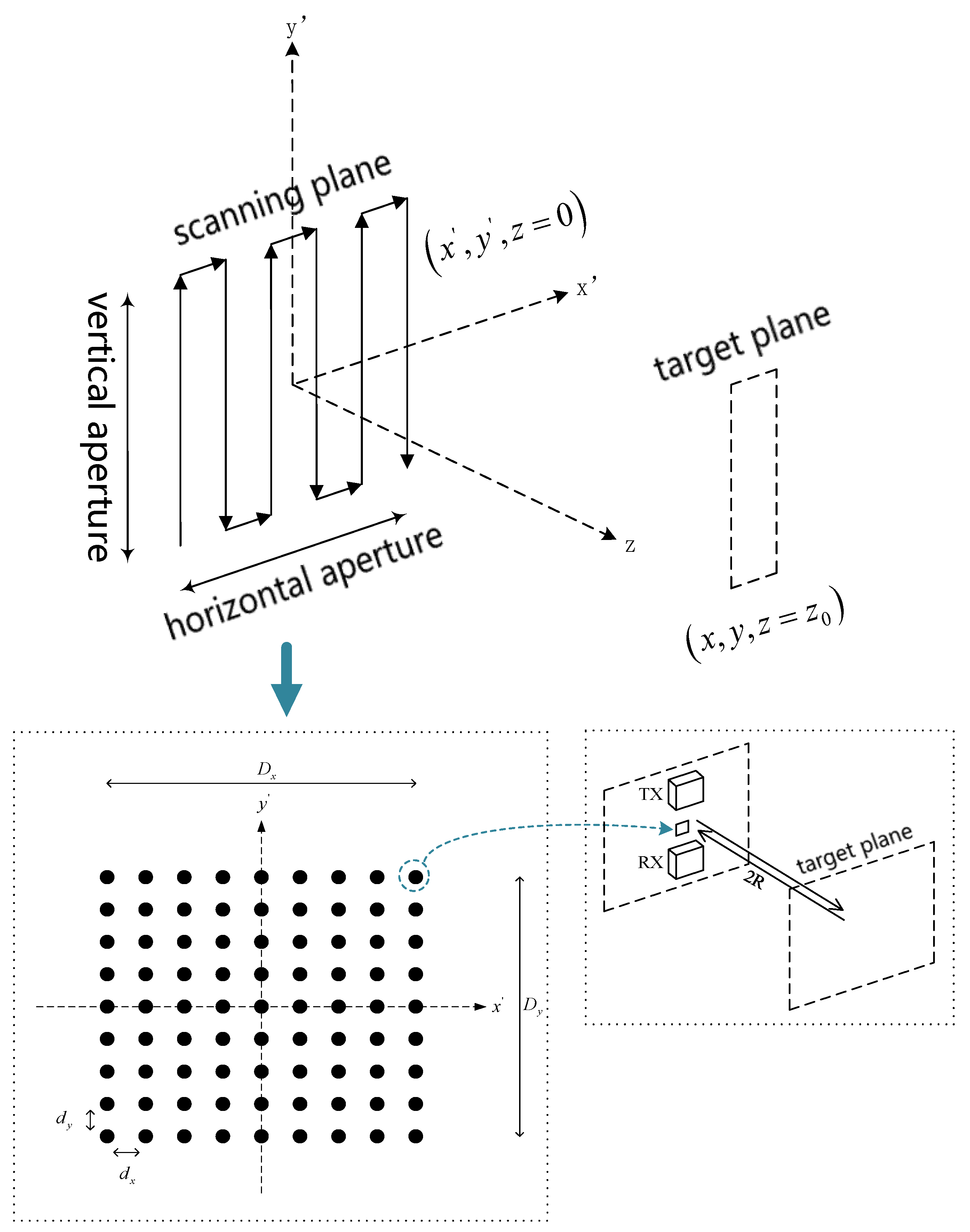Finally, we open mmWave Studio inside the upper computer and set up the parameters in Section 4.2.1, then open MATLAB and run the specially written program to set up the parameters in Section 4.2.2 according to the scene requirements. Once the setup is complete, the data capturing begins. In the process of capturing, the radar is first scanned along the columns, and after a column is fully scanned, it is then scanned one step along the rows, followed by the next column, and the final trajectory, as shown in the top of Figure 2. The scanning method used in this paper is discrete, i.e., “one move, one stop”, when stopping, the radar works and sends and receives signals, when moving, the radar does not work, and finally data are collected at each sampling point shown in the bottom left of Figure 2.

4.3.1. Single Target Imaging

(1) Fully-Sampled Single Target. In order to verify the feasibility of the mmSight, a single target is imaged with Fully-Sampled, the parameters are the same as those set in Section 4.2, the distance from the target plane to the array plane ($z_0$) is 110 mm, and the number of horizontal sampling points and vertical sampling points are both 41, so that the virtual aperture size is 80 mm × 80 mm, which can cover the target of size 60 mm × 60 mm. The optical image of the circle target is shown in Figure 6a, and the imaging results are shown in Figure 6c. It can be seen that the algorithm has high imaging quality for the circle target and accurate contour restoration. The star target optical image is shown in Figure 6b, and the imaging results are shown in Figure 6d. The star target is more complex than the circle target, and the algorithm, although the general outline is accurately restored, for the detailed part, the restoration is insufficient. In particular, the part connecting the periphery and the center is not well resolved in this part because its width is smaller than the spatial sampling interval (2 mm). In addition, there is a certain amount of spatial noise accompanying it.

(2) Sparsely-Sampled Single Target. Sometimes, to quickly verify the feasibility of the algorithm, it is necessary to image in the case of Sparsely-Sampled, but this produces ghost image, and the general research mostly uses the MIMO approach to avoid ghost image by converting Sparsely-Sampled under SISO to Fully-Sampled under MIMO, but MIMO increases the complexity of the system, so it is more necessary to study the avoidance of ghost image in the case of Sparsely-Sampled under SISO. Therefore, in this paper, based on the Fully-Sampled single-target imaging experiments, the rail parameters are modified and the corresponding Sparsely-Sampled experiments are performed. Figure 7 shows the horizontal and vertical directions are both Sparsely-Sampled (horizontal sampling interval and vertical sampling interval are 4 mm, which does not satisfy the spatial sampling criterion, the number of horizontal and vertical sampling points is 21, and the virtual aperture size is 80 mm × 80 mm, which can cover the target), where the mmSight (Figure 7a) gets the imaging effect close to fully-sampled and does not produce ghost image, while the Back Projection (Figure 7b) and Matched Filter (Figure 7c) imaging algorithms produce ghost image in the horizontal and vertical directions. Figure 8 shows the case of Sparsely-Sampled in the vertical direction only (horizontal sampling interval is 2 mm, vertical sampling interval is 4 mm, the number of horizontal sampling points is 41, the number of vertical sampling points is 21, the virtual aperture size is 80 mm × 80 mm, which can cover the target), where the mmSight (Figure 8a) obtained the imaging effect of nearly Fully-Sampled, which did not produce ghost image, and the Back Projection (Figure 8b), and Matched Filter (Figure 8c) imaging algorithms produced ghost image only in the vertical direction. In the case of Sparsely-Sampled, the mmSight is based on the Analytic Fourier Transform, compared to the Back Projection, Matched Filter, which effectively avoids the generation of ghost image.

4.3.2. Hidden Target Imaging

The mmSight, using the obtained echo data, solves the reflectivity of the object, so the stronger the reflectivity of the object’s material, the better the imaging effect, while the weaker the reflectivity of the object’s material, the worse the imaging effect, in order to verify this, the imaging experiment of the hidden target was conducted. Most of the parameter settings of this experiment are consistent with the first group of Section 4.3.1, but the number of horizontal sampling points and vertical sampling points are both set to 51, making the virtual aperture size of 100 mm × 100 mm, in addition to being able to cover the target, but also cover part of the carton. Figure 9a,b show the experimental scenarios, and Figure 9c shows the imaging results. From the results, it can be seen that the millimeter wave penetrated the carton and was reflected by the metal with a circle shape.

4.3.3. Multiple Targets Imaging

(1) Same-Distance Multiple Targets. In real scenarios, there are usually multiple targets, and making a distinction between multiple targets and imaging them separately and accurately is more complex than in a single-target scenario. In addition, more targets also require larger apertures, longer sampling times, and higher requirements for the stability of the system, making it necessary to conduct experiments related to multiple targets. Most of the parameter settings in this experiment are consistent with the first group in Section 4.3.1, but the distance ($z_0$) from the target plane to the array plane is 87 mm, the number of horizontal sampling points is 81 and the number of vertical sampling points is 41, making the virtual aperture size 160 mm × 80 mm, which can cover two targets. The multi-targets scenario, imaging results are shown in Figure 10. From the results, it can be seen that different targets are distinguished in the same distance plane. However, because the distance between the two planes (87 mm) was shortened than Section 4.3.1 Experiment one (110 mm), according to the literature [11] Equation (13), the interval of the spatial sampling criterion also became smaller, so the original sampling interval of 2 mm, does not meet the new sampling criterion requirements for the Back Projection (Figure 10b), Matched Filter (Figure 10c), results of them appeared unwanted spatial noise, while the Analytic Fourier Transform (Figure 10d) and the mmSight (Figure 10e) are unaffected and still maintain high-quality imaging results.

(2) Different-Distance Multiple Targets. For multiple targets in the same distance plane, only a large aperture needs to be set, but for targets in different distance planes, the algorithm often focuses on a single distance plane only, resulting in poor imaging of targets in other distance planes. In this regard, the literature [16,17] proposed the maximum projection approach to integrate targets from multiple planes, but this requires imaging for each plane and finally projection, which has more steps, while the mmSight in this paper can take into account multiple planes at once, which greatly reduces the workload compared to the projection method. Most of the parameters set in this experiment are consistent with the first group of Section 4.3.3. The distance from the plane where the star target is located to the array plane is 108 mm, while the distance from the plane where the circle target is located to the array plane is 135 mm, and the difference between the planes where the two targets are located is 27 mm, as shown in Figure 11a. The final results are shown on the right side of Figure 11. The mmSight (Figure 11e) can take into account the targets of other secondary distance planes, and the result, which is close to that of the dual targets of the same distance plane, is one of its advantages over the Analytic Fourier Transform (Figure 11d). In addition, since the inter-plane distance is 108 mm, which is farther than the 87 mm distance of the previous experiment, Back Projection (Figure 11b) and Matched Filter (Figure 11c), do not appear ghost image, but the residual spatial noise of them is still more.

In addition, we made a comparison with the work in literature [31,32], as shown in Figure 12, Figure 13, Figure 14 and Figure 15. Figure 12, the primary target is the metal sheet, and the secondary target is the bracket. From the results, it can be seen that mmSight images the bracket better than the other algorithms, but the projection is not as good as Figure 11e because of the large distance between the two targets, which exceeds the 27 mm set in the previous experiment. Figure 13 considers the hidden, different-distances projection problem together, and it can be seen that mmSight’s projection of the secondary target (top left, distance 260 mm) plane to the primary target (bottom right, distance 320 mm) plane is better than the other algorithms, but again, the projection is not as good as Figure 11e because of the larger distance difference (60 mm). Also, mmSight still outperforms the other algorithms for spatial noise cancellation. 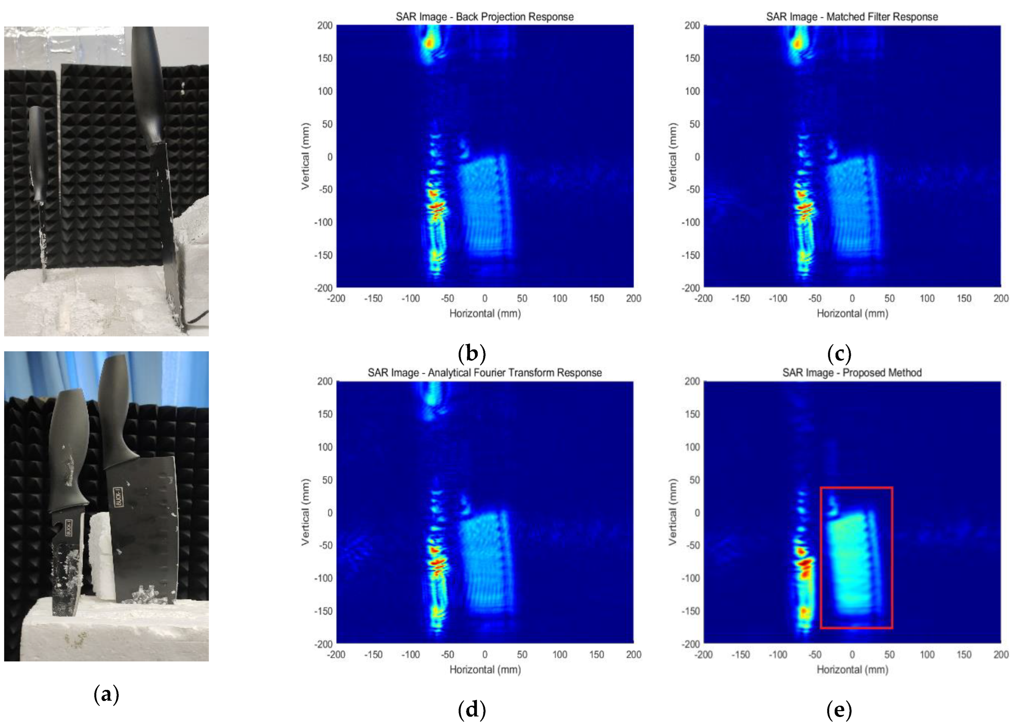Figure 14, the distance between the dagger (550 mm) and the knife (585 mm) is 35 mm. Figure 15, the distance between the pistol (550 mm) and the knife (600 mm) is 50 mm. This also shows that the larger the spacing is, the worse the projection effect is.

4.4. Experimental Evalution

In the field of image processing, a pixel is the smallest unit that constitutes an image, and accordingly, in the field of RF imaging, the point target imaging result is equivalent to a pixel and is the smallest unit that constitutes the imaging result, and the analysis of the point target contributes to the analysis of the imaging quality. Therefore, in this paper, the mmSight will be evaluated in terms of the Image Entropy (IE) and Point Spread Function (PSF) corresponding to the point target.

4.4.1. Point Target

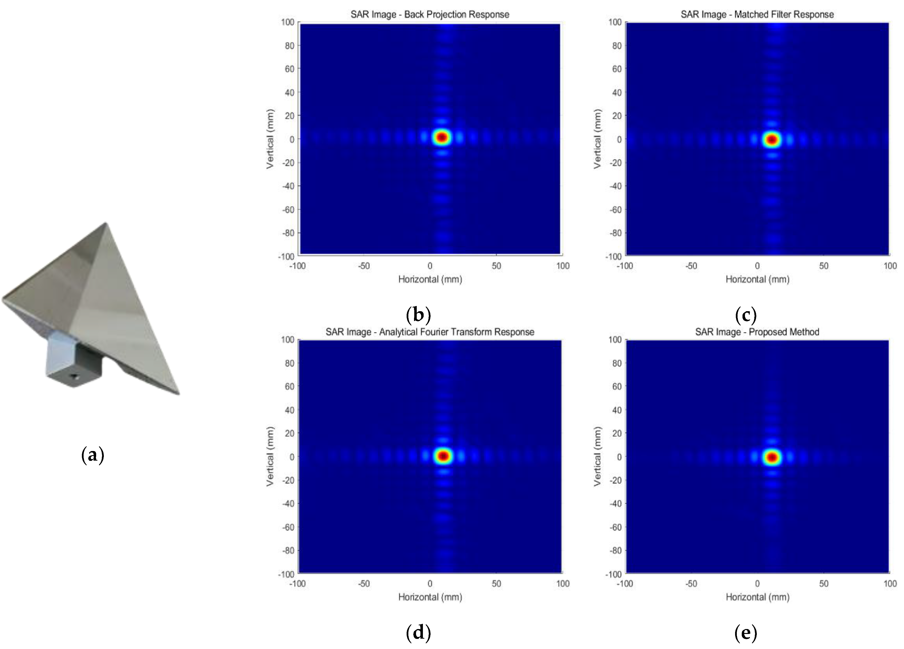
In this paper, a corner reflector is used as a point target, which is placed at a distance of 200 mm from the scanning plane, and other parameters are the same as experiment one in Section 4.3.1, and then imaging the corner reflector. The corner reflector is shown in Figure 16a. The obtained point target imaging results are shown on the right side of Figure 16.

4.4.2. Image Entropy

The quantitative evaluation is first performed using Image Entropy (IE), which is calculated as shown in Equation (16) [17], where $f(i,j)$ denotes the pixel of the reconstructed image. The smaller the entropy value, the better the focusing performance of the image, and the better the image quality.

$$IE=-{\displaystyle \sum _i{\displaystyle \sum _j\frac{{\left|f\left(i,j\right)\right|}^2}{{\displaystyle \sum _i{\displaystyle \sum _j{\left|f\left(i,j\right)\right|}^2}}}}}\ln \frac{{\left|f\left(i,j\right)\right|}^2}{{\displaystyle \sum _i{\displaystyle \sum _j{\left|f\left(i,j\right)\right|}^2}}}$$

(16)

Table 4. Image Entropy of point target (Using Formula (16) to calculate, the input is from Figure 16 and the output is IE).

Algorithm	Image Entropy
Back Projection	5.0076
Matched Filter	5.0089
Analytic Fourier Transform	4.8424
mmSight	4.6157

shows the Image Entropy corresponding to the target of Figure 16, from which it can be seen that the Proposed imaging algorithm has the best result, the Analytic Fourier Transform has the second best result, while Back Projection and Matched Filter have slightly worse results.

4.4.3. Point Spread Function

An evaluation is undertaken using the Point Spread Function (PSF), which is essentially the impulse response of the imaging system. The imaging algorithm can be evaluated by observing its trend of sidelobe change and the strength of the background noise. The larger the sidelobe, the more likely it is to produce ghost image; the stronger the background noise, the more useless information in the image.

The Point Spread Function can be obtained after normalizing the point target imaging results, and the results are shown in Figure 17, from which it can be seen that the differences among the four algorithms are mainly in the sidelobe. Among them, the sidelobe of the mmSight and the Analytic Fourier Transform decrease gradually from the main peak to the edge. The sidelobe of Back Projection and Matched Filter from the main peak to the edge, decreasing first and then increasing. In addition, the mmSight in this paper has the best suppression effect on edge-sidelobe, followed by Analytic Fourier Transform, Back Projection and Matched Filter are worse. This is also the reason why Back Projection and Matched Filter tend to produce a ghost image. Finally, it can be seen from the figure that the difference between the main peak amplitude and the background amplitude of the mmSight is large, so the spatial noise is effectively suppressed. Analytic Fourier Transform is the next best, while Back Projection and Matched Filter are worse.

5. Discussion and Future Work

5.1. Discussion

The experimental results show that mmSight performs better in near-field conditions compared to other algorithms. In the Fully-Sampled single-target experiment, we perform basic validation of mmSight, and the results show that it can achieve high-resolution imaging. In the Sparsely-Sampled single-target experiment, unlike the MIMO in most papers, this paper is under SISO. Comparing Matched Filter and Back Projection, mmSight effectively suppresses the ghost image, which can ensure the algorithm robustness. In the hidden target experiment, we verify the penetration ability of the millimeter wave and successfully achieve the target imaging inside the carton. In the same-distance multi-targets experiment, we verified the feasibility of multiple targets imaging, and then discussed the effect of the spacing distance on the generation of ghost image. The experiment verified the spatial sampling theory that the closer the spacing distance, the smaller the sampling interval required by the spatial sampling criterion, and the more likely to generate ghost image. In the multi-targets experiment at different distances, we spaced two targets 27 mm apart, and no other algorithms could achieve the same distance projection that mmSight did. Comparing the dataset used in the literature [31,32], we can see the advantages of mmSight in different distances multi-targets projection and low noise, but we can also see that the projection is limited to the spacing distance, and the larger the spacing distance, the worse the projection effect. For the index IE, the smaller the value, the higher the image quality. mmSight is lower than other algorithms by 0.3372 on average, which can prove that mmSight’s imaging quality is better than that of other algorithms. For the PSF’s sidelobe and noise, mmSight is also lower than other algorithms. In summary, mmSight is able to achieve robust, high-quality imaging.

5.2. Future Work

Although mmSight is superior to general imaging algorithms, there are still some problems. The present algorithm, like other conventional imaging algorithms, requires a large aperture array with uniform sampling interval to capture data. If a real aperture array is used, the hardware cost will be high and it is too complex to maintain, while using a synthetic virtual aperture, the capturing time is long and cannot meet the real-time requirements of many applications. In addition, the equipment required for both approaches would occupy a certain amount of space and would not be portable. A lot of work has been undertaken to address the miniaturization of imaging equipment with real-time and irregular sampling intervals. However, some work is done in exchange for reduced resolution, and some work needs to rely on outside devices like tags and positioning devices. Therefore, how to take into account the miniaturization of equipment and real-time, high resolution, no outside device-dependent, is still a future research direction of RF imaging.

mmSight is still a modification of the conventional algorithm, and the imaging results are essentially a distribution map of the target reflectivity, so it is still material-dependent. For targets with high reflectivity, such as metal, there will be good imaging results, while for targets with low reflectivity, such as carton, the imaging results are not ideal. Therefore, how to find a new feature to replace reflectivity and achieve material-independent imaging is also a future research direction for RF imaging. We can see the future direction from

Table 5. Future trend from related work.

Source	Device-Portable	Real-Time	High-Resolution	Out-Device Independent	Material-Independent
[4]	Yes	Yes	No	Yes	No
[33]	Yes	Yes	Yes	No	No
[34]	Yes	Yes	Yes	No	No

.

6. Conclusions

In this paper, we propose a millimeter wave near-field SAR imaging algorithm called mmSight. The original data are optimized using Blackman window, which facilitates the mapping of multiple targets at different distances. The optimized data are processed using Analytic Fourier Transform algorithm, which can effectively avoid ghost image. The imaging results are processed using mean filtering to remove spatial noise. The penetration of millimeter wave is used to achieve the detection of hidden targets. In the IE of point target imaging results, mmSight obtained a value of 4.6157, which is 0.2267 lower than the Analytic Fourier Transform, 0.3919 lower than the Back Projection, and 0.3932 lower than the Matched Filter. For PSF, mmSight’s sidelobe and noise are smaller than those of other algorithms. The experimental results show that mmSight can achieve robust, high-quality imaging under near-field conditions compared to other common SAR imaging algorithms. In the future, we hope to further promote the miniaturization of RF imaging devices, and further study real-time, high-resolution, no outside device-dependent, material-independent imaging, and further study the effect of irregular sampling on imaging, and try to further expand the application scope of millimeter wave imaging technology.

References

1. Heidari, A.; Navimipour, N.J.; Unal, M. Applications of ML/DL in the management of smart cities and societies based on new trends in information technologies: A systematic literature review. Sustain. Cities Soc. 2022, 85, 104089. [Google Scholar] [CrossRef]
2. Heidari, A.; Toumaj, S.; Navimipour, N.J.; Unal, M. A privacy-aware method for COVID-19 detection in chest CT images using lightweight deep conventional neural network and blockchain. Comput. Biol. Med. 2022, 145, 105461. [Google Scholar] [CrossRef] [PubMed]
3. Heidari, A.; Navimipour, N.J.; Unal, M.; Toumaj, S. The COVID-19 epidemic analysis and diagnosis using deep learning: A systematic literature review and future directions. Comput. Biol. Med. 2021, 141, 105141. [Google Scholar] [CrossRef] [PubMed]
4. Zhang, F.; Wu, C.; Wang, B.; Liu, K.J.R. mmEye: Super-resolution millimeter wave imaging. IEEE Internet Things J. 2020, 8, 6995–7008. [Google Scholar] [CrossRef]
5. Sheen, D.M.; McMakin, D.L.; Hall, T.E. Three-dimensional millimeter-wave imaging for concealed weapon detection. IEEE Trans. Microw. Theory Tech. 2001, 49, 1581–1592. [Google Scholar] [CrossRef]
6. Liu, J.; Zhang, K.; Sun, Z.; Wu, Q.; He, W.; Wang, H. Concealed object detection and recognition system based on millimeter wave fmcw radar. Appl. Sci. 2021, 11, 8926. [Google Scholar] [CrossRef]
7. Song, S.; Lu, J.; Xing, S.; Quan, S.; Wang, J.; Li, Y.; Lian, J. Near Field 3-D Millimeter-Wave SAR Image Enhancement and Detection with Application of Antenna Pattern Compensation. Sensors 2022, 22, 4509. [Google Scholar] [CrossRef]
8. Li, L.; Zhang, X.; Zhou, Y.; Pu, L.; Shi, J.; Wei, S. Region adaptive morphological reconstruction fuzzy C-means for near-field 3-D SAR image target extraction. Digit. Signal Process. 2021, 113, 103036. [Google Scholar] [CrossRef]
9. Cheng, Q.; Chen, G.; Wang, L.; Guan, C. Millimeter wave image object detection based on convolutional neural network. Sci. Technol. Eng. 2020, 20, 5224–5229. [Google Scholar]
10. Yanik, M.E.; Torlak, M. Near-field 2-D SAR imaging by millimeter-wave radar for concealed item detection. In Proceedings of the Radio and Wireless Symposium (RWS), Orlando, FL, USA, 20–23 January 2019; pp. 1–4. [Google Scholar]
11. Yanik, M.E.; Torlak, M. Millimeter-wave near-field imaging with two-dimensional SAR data. Proc. SRC Techcon. 2018, 1–5. [Google Scholar]
12. Gan, L.; Zhou, Z.; Shi, C.; Zhang, R. 2D Near-Field Imaging System for 24GHz Frequency Modulated Continuous Wave Radar. J. Microw. 2022, 38, 67–71. [Google Scholar]
13. Yanik, M.E.; Torlak, M. Near-field MIMO-SAR millimeter-wave imaging with sparsely sampled aperture data. IEEE Access 2019, 7, 31801–31819. [Google Scholar] [CrossRef]
14. Xia, Z.; Jin, S.; Yue, F.; Yang, J.; Zhang, A.; Zhao, Z.; Zhang, C.; Gao, W.; Zhang, T.; Zhang, Y.; et al. A Novel Space-Borne High-Resolution SAR System with the Non-Uniform Hybrid Sampling Technology for Space Targets Imaging. Appl. Sci. 2022, 12, 4848. [Google Scholar] [CrossRef]
15. Xue, B.; Zhang, G.; Leung, H.; Wang, L. An Applied Frequency Scaling Algorithm Based on Local Stretch Factor for Near-Field Miniature Millimeter-Wave Radar Imaging. IEEE Transactions on Microwave Theory Tech. 2022, 70, 2786–2801. [Google Scholar] [CrossRef]
16. Cai, J.; Yang, C.; Zhuo, Z. Millimeter Wave Near Field Imaging Algorithm Based on Range Compensation. J. Microw. 2021, 37, 6. [Google Scholar]
17. Yang, C.; Song, J.; Zhuo, Z. A Millimeter-Wave Near-Field Imaging Algorithm Based on Amplitude Compensation. Telecommunication Engineering: 1–6. Available online: http://kns.cnki.net/kcms/detail/51.1267.TN.20220915.1232.004.html (accessed on 19 November 2022).
18. Adib, F.; Hsu, C.Y.; Mao, H.; Katabi, D.; Durand, D. Capturing the human figure through a wall. ACM Trans. Graph. (TOG) 2015, 34, 1–13. [Google Scholar] [CrossRef]
19. Sun, Y.; Huang, Z.; Zhang, H.; Cao, Z.; Xu, D. 3DRIMR: 3D Reconstruction and Imaging via mmWave Radar based on Deep Learning. In Proceedings of the International Performance, Computing, and Communications Conference (IPCCC), Austin, TX, USA, 29–31 October 2021; pp. 1–8. [Google Scholar]
20. Wu, Z.; Zhang, D.; Xie, C.; Yu, C.; Chen, J.; Hu, Y.; Chen, Y. RFMask: A Simple Baseline for Human Silhouette Segmentation with Radio Signals. arXiv 2022, arXiv:2201.10175. [Google Scholar] [CrossRef]
21. Zhang, Y.; Deng, B.; Yang, Q.; Gao, J.; Qin, Y.; Wang, H. Near-field three-dimensional planar millimeter-wave holographic imaging by using frequency scaling algorithm. Sensors 2017, 17, 2438. [Google Scholar] [CrossRef] [Green Version]
22. Yanik, M.E.; Wang, D.; Torlak, M. 3-D MIMO-SAR imaging using multi-chip cascaded millimeter-wave sensors. In Proceedings of the Global Conference on Signal and Information Processing (GlobalSIP), Ottawa, ON, Canada, 11–14 November 2021; pp. 1–5. [Google Scholar]
23. Smith, J.W.; Torlak, M. Efficient 3-D Near-Field MIMO-SAR Imaging for Irregular Scanning Geometries. IEEE Access 2022, 10, 10283–10294. [Google Scholar] [CrossRef]
24. Zhang, R.; Cao, S. 3D imaging millimeter wave circular synthetic aperture radar. Sensors 2017, 17, 1419. [Google Scholar] [CrossRef]
25. Guo, Q.; Chang, T.; Cui, H.L. Three-dimensional millimeter wave imaging of borehole wall cracks. In Proceedings of the 43rd International Conference on Infrared, Millimeter, and Terahertz Waves (IRMMW-THz), Nagoya, Japan, 9–14 September 2018; pp. 1–2. [Google Scholar]
26. Zeng, S.; Fan, W.; Du, X. Three-Dimensional Imaging of Circular Array Synthetic Aperture Sonar for Unmanned Surface Vehicle. Sensors 2022, 22, 3797. [Google Scholar] [CrossRef] [PubMed]
27. Smith, J.W.; Yanik, M.E.; Torlak, M. Near-field MIMO-ISAR millimeter-wave imaging. In Proceedings of the Radar Conference (RadarConf20), Florence, Italy, 21–25 September 2020; pp. 1–6. [Google Scholar]
28. Jiang, L.; Wang, L.; Che, L. Automotive synthetic aperture radar imaging method for obtaining elevation information. Sci. Technol. Eng. 2021, 21, 6337–6344. [Google Scholar]
29. Guo, Q.; Li, C.; Zhou, T.; Li, H.; Huang, J. Millimeter-wave imaging using accelerated coherence factor based range migration algorithm. Optik 2020, 222, 165382. [Google Scholar] [CrossRef]
30. Texas Instruments. The Fundamentals of Millimeter Wave Radar Sensors. Available online: http://www.ti.com/sensors/mmwave/overview.html (accessed on 20 December 2018).
31. The University of Texas at Dallas. SAR IMAGING TUTORIAL. Available online: https://github.com/meminyanik/Simplified-2D-mmWave-Imaging (accessed on 20 April 2019).
32. Wei, S.; Zhou, Z.; Wang, M.; Wei, J.; Liu, S.; Shi, J.; Zhang, X.; Fan, F. 3DRIED: A High-Resolution 3-D Millimeter-Wave Radar Dataset Dedicated to Imaging and Evaluation. Remote Sens. 2021, 13, 3366. [Google Scholar] [CrossRef]
33. Alvarez-Narciandi, G.; Lopez-Portugues, M.; Las-Heras, F.; Laviada, J. Freehand, agile, and high-resolution imaging with compact mm-wave radar. IEEE Access 2019, 7, 95516–95526. [Google Scholar] [CrossRef]
34. Álvarez-Narciandi, G.; Laviada, J.; Las-Heras, F. Towards turning smartphones into mmWave scanners. IEEE Access 2021, 9, 45147–45154. [Google Scholar] [CrossRef]
Figure 1. Processing Flow (The left side is data capturing, realized by SAR; the right side is target imaging, which contains three steps of optimizing, imaging, and filtering).
Applsci 12 12085 g001
Figure 2. System Model (The motion trajectory of SAR in this paper is shown on the top; the synthesized virtual array is shown on the left below, and the monostatic is shown on the right. The interconnection between them is indicated by arrows).
Applsci 12 12085 g002
Figure 3. Radar Cube Data.
Applsci 12 12085 g003
Figure 4. Procedure of windowing.
Applsci 12 12085 g004
Figure 5. Experimental platform.
Applsci 12 12085 g005
Figure 6. Fully-sampled experiment: (a) Optical image of circle target; (b) Optical image of star target; (c) Imaging result of circle target; (d) Imaging result of star target.
Applsci 12 12085 g006
Figure 7. Horizontal direction and vertical direction sparsely-sampled: (a) mmSight; (b) Back Projection; (c) Matched Filter.
Applsci 12 12085 g007
Figure 8. Vertical direction sparsely-sampled only: (a) mmSight; (b) Back Projection; (c) Matched Filter.
Applsci 12 12085 g008
Figure 9. Hidden target: (a) outside; (b) inside; (c) imaging result.
Applsci 12 12085 g009
Figure 10. Same-Distance multiple targets: (a) real scenario; (b) Back Projection; (c) Matched Filter; (d) Analytic Fourier Transform; (e) mmSight.
Applsci 12 12085 g010
Figure 11. Different-Distance multiple targets: (a) scenario; (b) Back Projection; (c) Matched Filter; (d) Analytic Fourier Transform; (e) mmSight.
Applsci 12 12085 g011
Figure 12. Different-Distance multiple targets: (a) scenario-1; (b) Back Projection; (c) Matched Filter; (d) Analytic Fourier Transform; (e) mmSight (red frame: projection of other target).
Applsci 12 12085 g012
Figure 13. Hidden and Different-Distance multiple targets: (a) scenario; (b) Back Projection; (c) Matched Filter; (d) Analytic Fourier Transform; (e) mmSight (red frame: projection of other target).
Applsci 12 12085 g013
Figure 14. Different-Distance multiple targets: (a) scenario-2; (b) Back Projection; (c) Matched Filter; (d) Analytic Fourier Transform; (e) mmSight (red frame: projection of other target).
Applsci 12 12085 g014
Figure 15. Different-Distance multiple targets: (a) scenario-3; (b) Back Projection; (c) Matched Filter; (d) Analytic Fourier Transform; (e) mmSight (red frame: projection of other target).
Applsci 12 12085 g015
Figure 16. Point target: (a) corner reflector; (b) Back Projection; (c) Matched Filter; (d) Analytic Fourier Transform; (e) mmSight.
Applsci 12 12085 g016
Figure 17. Point Spread Function: (a) Back Projection; (b) Matched Filter; (c) Analytic Fourier Transform; (d) mmSight.
Applsci 12 12085 g017aApplsci 12 12085 g017b