Article

Improving the Robustness and Quality of Biomedical CNN Models through Adaptive Hyperparameter Tuning

1
Faculty of Information Technology, Beijing University of Technology, Beijing 100124, China
2
Department of Computer Science, Faculty of Information Technology & Computer Science, University of Central Punjab, Lahore 54000, Pakistan
3
Beijing Engineering Research Center for IoT Software and Systems, Beijing 100124, China
4
Division of Science and Technology, University of Education, Lahore 54000, Pakistan
*
Authors to whom correspondence should be addressed.
Appl. Sci. 2022, 12(22), 11870; https://doi.org/10.3390/app122211870
Submission received: 25 October 2022 / Revised: 16 November 2022 / Accepted: 17 November 2022 / Published: 21 November 2022
(This article belongs to the Section Computing and Artificial Intelligence)

Abstract

:
Deep learning is an obvious method for the detection of disease, analyzing medical images and many researchers have looked into it. However, the performance of deep learning algorithms is frequently influenced by hyperparameter selection, the question of which combination of hyperparameters are best emerges. To address this challenge, we proposed a novel algorithm for Adaptive Hyperparameter Tuning (AHT) that automates the selection of optimal hyperparameters for Convolutional Neural Network (CNN) training. All of the optimal hyperparameters for the CNN models were instantaneously selected and allocated using a novel proposed algorithm Adaptive Hyperparameter Tuning (AHT). Using AHT, enables CNN models to be highly autonomous to choose optimal hyperparameters for classifying medical images into various classifications. The CNN model (Deep-Hist) categorizes medical images into basic classes: malignant and benign, with an accuracy of 95.71%. The most dominant CNN models such as ResNet, DenseNet, and MobileNetV2 are all compared to the already proposed CNN model (Deep-Hist). Plausible classification results were obtained using large, publicly available clinical datasets such as BreakHis, BraTS, NIH-Xray and COVID-19 X-ray. Medical practitioners and clinicians can utilize the CNN model to corroborate their first malignant and benign classification assessment. The recommended Adaptive high F1 score and precision, as well as its excellent generalization and accuracy, imply that it might be used to build a pathologist’s aid tool.

1. Introduction

One of the most typical deep learning algorithms is Convolutional Neural Networks (CNN). In recent decades, significant advancements in computer-aided diagnosis have been made thanks to the significant usage of CNNs in several domains of medical image analysis. A deep learning algorithm converts a problem into an improvement issue and solves the difficulty of using various optimization approaches. The improvement function is made up of a large number of hyperparameters that are defined before the learning process and influence how well the deep learning algorithm fits the model to the data. Internal CNN model parameters, such as the weights of a neural network, may be learned from the data during the model training phase, but hyperparameters are not. We want to identify a set of hyperparameter values that generate the greatest moment on the data in a fair length of time before we start the training phase. This is referred to as hyperparameter adjustment or optimization. It is critical to the accuracy of deep learning algorithms’ predictions. Furthermore, there is no apparent link between deep learning computational efficiency and hyperparameters. It is required to tweak a large number of hyperparameters on a regular basis and train various CNN models with various combinations of hyperparameters values, then compare model performance to select the optimal model. As a result, how to maximize hyperparameters in a deep learning algorithm becomes a critical topic [1].
Manual adjustment of deep learning models is feasible, but it is extremely reliant on the user’s knowledge and understanding of the key problem. Manual tweaking may still be impossible due to variables such as time-consuming model assessments and non-linear hyperparameter correlations among dozens or even hundreds of hyperparameters in complex models. This schematic design of defining model hyperparameters has been highlighted as an issue that impedes the adoption of deep learning approaches in AI-related challenges, prompting greater research into algorithms for performing autonomous hyperparameter optimization [1]. Furthermore, improvements in performance for certain benchmark issues have been observed not just from the introduction of brand-new, original deep learning models, but also from the discovery of superior hyperparameter combinations for existing models.
Manual search and automated search techniques are the two basic types of hyperparameter optimization approaches. Manual search is a method of manually tweaking and testing hyperparameter settings. It is based on the basic intuition and expertise of professional users who can discover the crucial elements that have a stronger influence on the outcomes and then utilize visualization tools to evaluate the link between specific hyperparameters and final outputs. Manual searching necessitates a greater sense of competence learning and technical expertise on the part of the user. It is also difficult for non-expert users to apply. Optimizing hyperparameters is a difficult task to repeat. Furthermore, as the number of hyperparameters and the list of values grows, it becomes exponentially more difficult, since individuals are not adept at dealing with high-dimensional data and are prone to misinterpreting or overlooking patterns and correlations in hyperparameters [2].
In the search for an automated method of hyperparameter tuning, the process of picking the best hyperparameter for a deep learning model is frequently stated as a Black Box Optimization (BBO) issue. No inherent component of the deep learning model’s assessment is taken into account in this scenario. As a result, the CNN is viewed as an undetermined optimization problem that translates a collection of hyperparameters to a performance score, which is the only data in the optimization algorithm. The problem is also stated to be of a global type since the optimization problem cannot be guaranteed to be convex due to the unstable nature of the mapping. Given the possibility of several local optima, most optimization techniques for global issues in deep learning models include a mechanism for balancing the exploration of new regions in the input space against the exploitation of previously high-quality solutions.
Automatic search strategies, such as Grid Search (GS) [3] or Cartesian product based hyperparameter search has been developed to solve the limitations of a manual search. Grid Search works on the premise of thorough searching. Grid Search educates a deep learning model on the training sample with all possible hyperparameters and its list of values and assesses its achievement on a cross-validation set using a preset measure. Finally, grid search generates hyperparameters with the best results. Although this method obtains automatic tuning and can potentially obtain the global optimal value of the optimization accusative function, it undergoes the dimensionality curse, which means that the algorithm’s efficiency declines as a large number of hyperparameters and its list of values being optimized and the scope of hyperparameter values increases.
The Random Search method [3] was suggested to overcome the problem of high computational cost in a grid search, and it was discovered that only a few of the hyperparameters are truly relevant for most data sets. Limiting the examination to non-essential hyperparameters, the overall efficiency may be increased, and the model equation of the optimization function can be achieved. Random search tries a variety of value possibilities at random. It is more efficient in a high-dimensional space than Grid Search [4]. Random search, on the other hand, is unsatisfactory for training some complicated CNN models, as reveals [3].
As a result, getting the automated optimization technique to attain high precision and accuracy has always been an issue in deep learning that has not been entirely solved. A hyperparameter tweaking problem is one in which the optimization goal function is unknown or a black-box function. Conventional optimization approaches such as the Newton’s method and gradient descent are ineffective. In this type of optimization issue, Bayesian optimization is a very successful optimization approach [5]. Using the Bayesian formula, it incorporates prior knowledge about the unknown function of the population parameters to produce posterior knowledge about the function probability. Then, using this posterior data, we can figure out where the function gets its best value. The Bayesian optimization technique beats other global optimization methods in experiments [6]. As a result, we proposed the Adaptive Hyperparameter Tuning method based on Bayesian optimization and on the Gaussian process to adjust deep learning hyperparameters. If we assume that the optimization function follows a Gaussian distribution, we may calculate the prior distribution of hyperparameters. The Bayesian optimization approach is based on the Gaussian process will be presented in depth in the following sections. The proposed mechanism is then tested on the proposed CNN Deep-Hist [7] and on three different pretrained deep learning models such as ResNet, DenseNet, and MobileNetV2 to see if it works.
Fourfold contributions are evaluated in this work. First, the main theme of this study is to propose Adaptive Hyperparameter Tuning (AHT) for the selection of optimized hyperparameters to classify and analyze medical images. Second, we present a unique stable CNN model for healthcare image classification that incorporates the benefits of the Separable Convolution with a residual learning framework (ResNet) to enhance the exchange of knowledge and development ease. Third, we provide CNN model settings—providing a combination of hyperparameters with fewer parameters, cheaper space and quicker classification, making them more acceptable for healthcare applications. Fourth, we show that optimization algorithms can be effectively used to create CNN categorization designs.
We used medical image datasets such as BreakHis [8], BraTS [9], COVID-19 X-ray [10] and NIH X-ray [11] utilizing freely available information and pretrained CNN models such as ResNet, DenseNet and MobileNetV2. Almost all CNN hyperparameters are automatically tuned by the proposed Adaptive Hyperparameter Tuning (AHT) algorithm. The first task is to optimize the hyperparameters of the pretrained CNN models for image classification using the medical image dataset as BreakHis [8], BraTS, COVID-19 X-ray, and NIH X-ray. The second task involves optimizing the hyperparameters of a proposed neural network model for modeling using the medical imaging datasets. This study uses various medical imaging modalities such as BraTS for brain cancer, an X-ray of COVID19 and Histopathological images (BreakHis) of Breast Cancer. These modalities cover the most critical diseases and spread all over the world. The most recent state-of-the-artwork of Hyperparameter Optimization is reviewed in Section 2. In Section 3, we explain the basic preprocessing methodologies and provide the detailed thinking and implementation of the proposed Adaptive Hyperparameter Tuning (AHT) model. Section 5 comprises the training and testing results of various hyperparameters on three different medical imaging modalities and datasets. The final Section 6 concludes this study.

2. Related Work

A CNN model’s hyperparameters are the parameters that remain constant throughout the learning process and control the model’s speed and computational cost, including its efficiency and assessment of learning new data. These parameters regulate the strength of specific methods such as regularization parameters, namely the probability of nullified neurons using dropout value, using many hidden layers decide the model size and the learning rate regulates the stochastic gradient descent algorithm.
There are several types of hyperparameters such as integer, categorical and non-ordinal discrete. The hyperparameters of the CNN model are kernel size, stride size, pooling value, number of hidden layers, activation functions, learning rate, batch size, etc. The tuning of hyperparameters must now be formulated as an optimization issue. A maxima of an objective function O(f) concerning the variable f is sought in the general case of optimization. The problem is expressed mathematically as
min f R D O ( F )
For proper formulation, the hyperparameter selection as an optimization problem, certain an explanation must be made.
F = f c + f i + f l , f c = [ f 1 c , f 2 c , f 3 c , , f n c ] T R c : f i i c < f i c < f i x c f i = [ f 1 i , f 2 i , f 3 i , , f n i ] T Z i : f i i i < f i i < f i x i f l = [ f 1 l , f 2 l , f 3 l , , f n l ] T : f i l L i
The depicted Equation (2) explains the categorical hyperparameters as a f l , continuous hyperparameters as a f c and integer type hyperparameters as a f i , where f i i c and f i x c shows the minimum and maximum values of continuous and integer type hyperparameters respectively, the total dimension of the hyperparameter is depicted in F .

2.1. Hyperparameter Tuning

Hyperparameters are the trainable variables of a deep learning model which has some defined ranges. Everyone needs an optimal configuration of hyperparameter values to acquire satisfactory results from a deep learning model.
For obtaining satisfactory results from a deep learning model, we have to intelligently fine-tune different hyperparameters which is quite a tedious task and trivial task. Acquiring satisfactory results from a deep learning model, we manually set a different combination of hyperparameter values and it takes a lot of experience, good intuitions and vast knowledge regarding deep learning models. The most widely used hyperparameters are listed in Figure 1.
In the literature, there are different ways of tuning the hyperparameter values such as GridSearch, RandomSearch, and Bayesian Optimization (BO).

2.1.1. Grid Search

In this approach, we manually specified all the possible hyperparameters with real values and some have unbounded values. It means that every possible combination will be tried and compared with all the acquired results. This algorithm is guided by performance metrics to obtain the optimal configuration of hyperparameters. Curse of dimensionality the issue arose in Grid Search when we added more hyperparameters and time complexity exponentially increased. Hyperparameters define the dimensions of a Grid Search and values of each hyperparameter define the size of the dimension.

2.1.2. Random Search

In random searches, there is no guarantee to acquire the optimal configuration of hyperparameters, because it randomly selects the hyperparameter values and runs multiple tasks at the same time. It gives better results with high dimensions in less time. Both approaches have the independent guess issue, each new guess is autonomous from the previous one.

2.2. State of the Art

A wide range of hyperparameter optimization methodologies has recently developed. We only examine supporting structures for hyperparameter optimization because of space limits, and we ignore alternative methodologies for generic AutoML, including Auto-Sklearn [12] and AutoGluon [13]. Ray Tune [14] which employs Ray [15] as the back-end to spread the hyperparameter optimization process, is perhaps the most comparable to SyneTune. RayTune can run a variety of hyperparameter optimization techniques, but it cannot conduct multi-objective optimization, restricted maximization, transfer learning and evaluation.
Tree Parzen Estimator approach [4], Covariance Matrix Adaptation-Evolution Strategy (CMA-ES) [16], and even multi-objective optimization are all supported by Optuna [17], but are not contemporary multi-fidelity techniques such as Asynchronous Successive Halving Algorithm (ASHA) [18] and Population Based Training (PBT) [19]. SMAC3 [20] supports multi-fidelity methods such as Bayesian Optimization using Hyperband (BOHB) [21] and Hyperband [22]; however, these are not multi-objective or restricted optimization methods. It also lacks support for asynchronous parallel methods like neural network incremental backups and asynchronous scheduling. Dragonfly [23] supports decentralized-based hyperparameter optimization techniques, but not multi-objective or transfer learning situations. HyperTune [24] has several asynchronous multi-fidelity techniques based on successive halving; however, it does not enable decentralized tweaking across several computers or provide integrated benchmarks for large-scale investigations that can be replicated. Bayesian Optimization libraries such as BOTorch, are loosely linked [25]. However, rather than decentralized hyperparameter optimization, their primary goal is to provide a framework for Monte Carlo bayesian optimization research.
Hyperparameter optimization has been effectively implemented using Bayesian optimization (BO) [26]. Hyperband [22] automatically assigns resources to a collection of arbitrary combinations and employs the consecutive halving technique [27] to end poorly-performing combinations in advance, rather than using comprehensive evaluations. Bayesian optimization-based hyperband [21] enhances hyperband by using Bayesian optimization instead of random sampling. Two techniques [28,29] suggest using learning curve extrapolation to advise early halting. A median stopping criterion is also included in Vizier [30], RayTune [14], and OpenBox [31] to halt the assessments early. Furthermore, multi-fidelity approaches [32,33] use moderate data from partial evaluations to drive the search for the best objective function F . MFES-HB [33] blends hyperband with a Bayesian optimization based on multi-fidelity surrogates.
Various approaches [34,35] may analyze multiple combinations simultaneously rather than progressively. Furthermore, most of them [35], including BOHB [21] are focused on creating groups of configurations to analyze all at once, and just a handful offer asynchronous scheduling. Asynchronous evaluation methodology based on sequential halving method [27] is introduced by ASHA [18]. Furthermore, many asynchronous parallel computation techniques [36] cannot utilize multiple objective fidelity; A-BOHB [37] provides asynchronous multi-fidelity hyperparameter adjustment. A frequent tuning application for neural networks is searching for architectural hyperparameters. Recent empirical investigations [38] indicate that sequential Bayesian optimization methods [39,40] outperform a variety of Neural Architecture Search (NAS) approaches [41,42] emphasizing the need for parallelization-based bayesian optimization methods.
There are two types of comprehensive evaluation-based optimization and partially based optimization methods, Bayesian optimization [43], rule-based search, genetic algorithm [44], random search [45], and other autonomous hyperparameter optimization approaches exist. Complete evaluation-based techniques [3] need comprehensive evaluations, which are often computationally costly, to derive the performance for each configuration. Instead, partial evaluation-based approaches [21,22,33] allot each combination of various hyperparameters with incomplete training resources to acquire the evaluation result, hence conserving assessment resources.
In order to identify Diabetic Maculopathy in retinal pictures, this research examines the effects of applying the Bayesian optimization (BO) technique on the classification results of deep neural networks. In this study, they present two major customized CNN models for detecting Diabetic Maculopathy in datasets from fundus retinography and optical coherence tomography (OCT), two different forms of retinal imaging. The best designs for the suggested CNNs are chosen, and associated hyperparameters are optimized, using the Bayesian optimization technique. The results of this work show that the efficiency of the suggested CNNs for the categorization of diabetic maculopathy in retina and OCT images may be improved by utilising Bayesian optimization to fine-tune the network hyperparameters [46].
Using the most recent developments in deep learning, techniques utilizing transfer learning have succeeded in solving this challenge. Hyperparameter settings, meanwhile, are a prevalent issue when using deep learning techniques. To identify COVID19 using X-ray pictures, we used a transfer learning-based classification technique that we modified and expanded in this study. We also used a variety of optimization strategies to handle the hyper-parameter configuration problem [47].
The momentum is often controlled by a fixed in conventional CNN optimization techniques. However, momentum hyperparameter optimization can be substantially challenging. They provide a unique adaptive momentum for quick and reliable settlement in this work. The use of adaptive momentum frequency reduces the necessity for momentum hyperparameter adjustment by proposing raising or reducing based on variations in each epoch’s output [48].
Consequently, a strong technique for aiding doctors in taking medical decisions has appeared: deep learning-based human-centric scientific diagnostics. To automatically recognize Everything in blood pictures, various computer-aided diagnostic techniques have been created. For the purpose of detecting ALL in micro smear pictures, a novel Bayesian-based optimised CNN is presented in this paper. The design of the presented CNN as well as its hyperparameters are tailored to the raw data using the Bayesian optimization technique to improve classification efficiency. In order to find the number of network hyperparameters that minimizes an objective error measure, the Bayesian optimization approach employs an educated continuous search process [49].

3. Proposed Methodology

The proposed algorithm depicted in Figure 2 is based on the hyperparameter optimization algorithm Surrogate Model (SM), Acquisition Function (AF), and Tree Parzen Estimator (TPE). When resolving a complicated issue, a penalty-based boundary intersection decomposition strategy is chosen because it gives equally scattered alternatives on the perimeter areas of the Pareto Front and has a limited handful of weight vectors. This is significant in our scenario since training CNN models are strongly non-convex optimization issues, and the AHT-based learning model uses a limited amount of weight matrix to minimize computing complexity. On the other hand, the penalty-based boundary intersection technique, necessitates the determination of a compensation element to optimize the uniformity and variability of the results. On the BraTS MRI and BreakHis dataset, we used the AHT algorithms with 10 lists of hyperparameters with different ranges and with penalty component settings of 0.25, 0.5, 0.75, 1, 3, 5, 7, and 10 for the proposed Deep-Hist neural network. Component 7 was chosen since it gave a varied collection of responses that performed significantly in the optimal solutions. This penalty component has also been utilized in other experiments with positive outcomes. The intensities of the optimization methods can vary in numerous situations. A normalizing procedure is required in these circumstances to approach the optimization method’s output to a similar magnitude and reduce biases while choosing non-dominated spots. This normalization is critical in the suggested methodology since the accuracy and F1-Score yield values between [0→1], whereas the range of learnable parameters in a system might easily reach thousands.
Adaptive Hyperparameter Tuning (AHT) steps for determining the best Hyper settings are as follows:
In this approach, to find the optimal hyperparameters of deep learning algorithms that bring back the plausible performance. The representation of hyperparameter optimization is depicted in Equation (3).
ϰ * = arg min F ( ϰ )
ϰ * depicts the optimized hyperparameters list that predicts the lowest error, F which is an objective function to minimize the error (Root Mean Squared Error (RMSE)). In this approach, there is a surrogate function that optimizes the objective function on each iteration and selects the next hyperparameter.
The objective function ( F ( ϰ ) ) is the main evaluator that finds the optimal set of hyperparameters. Generally, It takes a simple set of hyperparameters and returns a negative score and according to the returned score, the set of hyperparameters will adjust for the next iteration.
Using the surrogate function, we can approximate the objective function by proposing parameters to the objective function. A Gaussian Process (GP) depicted in Equation (4) is simply a specific term for a method that takes two values in the input vector, ϰ and ϰ , as an argument and determines how “related” they are depending on a certain idea of “connection.” Tree Parzen Estimator (TPE – depicted in Equation (5)) and Random Forest Regression (RFR).
k ( x , x ) = σ 2 exp 1 2 2 x x 2
where ϰ ϰ then k ( ϰ , ϰ ) 0 . The duration of the swivels is determined by the factor. Usually, it will not be possible to estimate greater than units from the empirical observations. Similarly, the σ establishes our function’s total difference from its mean value. In short, σ and define the function’s horizontal and vertical domains.
t p e ( η ϰ ) = p ( ϰ η ) p ( η ) p ( ϰ ) t p e ( ϰ ( η ) ) = l ( ϰ ) i f η < η * g ( ϰ ) i f η η * E I η * ( ϰ ) = η * ( η * η ) p ( η ϰ ) d ( η ) = η * ( η * η ) p ( ϰ η ) p ( η ) p ( ϰ ) d ( η )
τ = p ( η < η * ) p ( ϰ ) = F p ( ϰ η ) p ( η ) d ( η ) = τ l ( ϰ ) + ( 1 τ ) g ( ϰ ) α = τ η * l ( ϰ ) l ( ϰ ) η * p ( η ) d ( η ) τ l ( ϰ ) + ( 1 τ ) g ( ϰ ) β = τ + g ( ϰ ) l ( ϰ ) ( 1 τ ) E I η * ( ϰ ) = α β 1
Upper Confidence Bound (UCB) comprises explicit exploitation μ ( ϰ ) and exploration σ ( ϰ ) components and is perhaps as straightforward as an acquisition function can acquire (7).
a ( ϰ ; λ ) = μ ( ϰ ) + λ σ ( ϰ )
The exploitation vs. exploration decision is simple and easier to tweak with upper confidence bound via the hyperparameter λ . The upper confidence bound is a weighted total of the anticipated efficiency recorded by μ ( ϰ ) the Gaussian Process and the ambiguity represented by the gaussian process’s standard error σ ( ϰ ) . When λ is modest, AHT will favor alternatives that are likely to function well, i.e., have a large μ ( ϰ ) . On the opposite, when λ is big, AHT encourages the discovery of previously unexplored portions of the solution space.
The Surrogate Model (SM) and the Acquisition Function (AF) are critical components of an Adaptive Hyperparameter Tuning (AHT) proposed algorithm. Surrogate models are frequently Gaussian Processes (GP) that can accommodate recorded datasets while quantifying the ambiguity of unseen regions. As a result, the surrogate model is to attempt to estimate the mysterious black-box function F ( ϰ ) . The AF then “reviews” the surrogate model to identify which regions of the scope of F ( ϰ ) are worthy of utilizing and which regions are worth investigating. As a result, the acquisition function has a great premium in locations in which F ( ϰ ) is ideal, or in regions where we have still not examined. On the opposite, the acquisition function expected score is modest in places where F ( ϰ ) is unsatisfactory or where we have recently tested. We determine the next wild estimate F ( ϰ ) to attempt by identifying the ϰ that maximizes the AF instead of explicitly maximizing F ( ϰ ) , whose analytical version we do not know, we instead maximize the acquisition function which is considerably simpler to perform and significantly less costly.
From the above mentioned algorithms, we apply the Tree Parzen Estimator, and the output of the algorithm is forward to the selection function. In this step, three common algorithms (Probability of Improvement (PI), Lower/Upper Confidence Bound (L/UCB), and Expected Improvement (EI)) are used for calculating expected improvements. The mathematical calculation of the most commonly used algorithm is depicted in Equation (8).
We want to maximize f( ϰ ), and the best option we have so far is ϰ . Then we can describe “improvement,” I( ϰ ) in Equation (8). As a result, if the incoming ϰ we are considering has an underlying quantity f( ϰ ) that is smaller than f( ϰ * ), f( ϰ ) − f( ϰ * ) is negligible. Therefore, we are not getting any better, because the above calculation produces 0 because the largest amount among any negative integer and 0 is 0. If the revised number f( ϰ ) is greater than our present best guess, then f( ϰ ) − f( ϰ * ) is optimistic. If we analyze f at the new location ϰ , I( ϰ ) yields the change, which is how significantly we will enhance our existing best answer.
I ( ϰ ) = max ( f ( ϰ ) f ( ϰ * ) , 0 ) P I = C D F ( μ μ * ν )
where CDF is the cumulative probability function, μ is the average of surrogate function, μ * shows the optimal average of the surrogate function founds so far, and ν is the standard deviation of the surrogate function.
Exploitation (evaluating at locations where the surrogate mean is low) and exploration (evaluating at sites where the surrogate variance is less) are trade-offs in acquisition functions. The employed acquisition function O(F) is optimized over the surrogate model to determine the next hyperparameters to assess. (In this case, f = arg min O ( F ) and F is the new hyperparameter value.) We add probabilistic modules in one of the most commonly utilized acquisition functions in the literature is the Probabilistic Expected Improvement Criterion. Expected Improvement (EI) is given as:
P E I = E P ( 0 , μ P ( f o p t O ( f ) ) )
where
Z = μ P ( f o p t ) O ( f ) ξ σ ( f ) if σ ( f ) > 0 0 if σ ( f ) = 0
In the end, we leveraged the assumption that the PDF of a normally distributed is symmetrical, therefore θ ( η 0 ) = θ ( η 0 ) ). Therefore, this equation may appear frightening, but it is not. So, whenever would EI(x) take on a bigger number and when μ f ( ϰ * ) . That is, the Gaussian Process’s average value is large at ϰ . When there is a bunch more ambiguity, the expected improvement increases, so when σ > 1. Through the meantime, the equation above applies for σ ( ϰ ) 0 ; alternatively, if σ ( ϰ ) = 0 (as at the recorded data points), EI( ϰ ) = 0. While we go, there is one more thing. We can smooth the AHT algorithm’s exploitation vs. exploration by inserting a (hyper)parameter(F) into the equation for EI(x). Therefore, the complete equations are (11) and (12).
EI ( ϰ ) E I ( ϰ ) = η * I ( ϰ ) φ ( η ) d η φ ( η ) = 1 2 π exp η 2 / 2
EI ( ϰ ) = η 0 max ( f ( ϰ ) f ( ϰ * ) , 0 ) φ ( η ) d η = η 0 μ + σ η f ( ϰ * ) φ ( η ) d η τ 1 = η 0 μ f ( ϰ * ) φ ( η ) d η = τ 1 + η 0 σ η 1 2 π e η 2 / 2 d η τ 1 = μ f ( ϰ * ) η 0 φ ( η ) d η 1 Φ ( η 0 ) 1 CDF ( η 0 ) = τ 1 + σ 2 π η 0 η e η 2 / 2 d η τ 1 = μ f ( ϰ * ) ( 1 Φ ( η 0 ) ) = τ 1 σ 2 π η 0 e η 2 / 2 d η τ 1 = μ f ( ϰ * ) ( 1 Φ ( η 0 ) ) = τ 1 σ 2 π e η 2 / 2 η 0 τ 1 = μ f ( ϰ * ) ( 1 Φ ( η 0 ) ) Φ ( η 0 ) = τ 1 + σ φ ( η 0 ) = μ f ( ϰ * ) Φ μ f ( ϰ * ) σ + σ φ μ f ( ϰ * ) σ τ 1 = μ f ( ϰ * ) F Φ μ f ( ϰ * ) F σ τ 2 = σ φ μ f ( ϰ * ) F σ EI ( ϰ ; ξ ) = τ 1 + τ 2
where f o p t shows the optimized hyperparameter values, and μ P ( f o p t ) is the posterior mean. μ ( f ) and σ ( f ) are the mean and the standard deviation of the GP posterior predictive at f , respectively. Φ and ϕ are the CDF and PDF of the standard normal distribution, respectively.
The depicted Figure 1 has list of hyperparameters “nu” as numbers of Neurons, “af” as Activation Functions (‘relu’, ‘sigmoid’, ‘softplus’, ‘softsign’, ‘tanh’, ‘selu’, ‘elu’, ‘exponential’, LeakyReLU, ‘relu’), “opt” as Optimizer (‘SGD’, ‘Adam’, ‘RMSprop’, ‘Adadelta’, ‘Adagrad’, ‘Adamax’, ‘Nadam’, ‘Ftrl’, ’SGD’) “lr” as learning rate (0.01–1), bs as Batch Size (4–256), ep as epochs (20–100), lyr as layers (1–3), norm as Normalization (0–1), drop as the drop-out rate (0–0.3) and k as Kernel (3–9).
For getting optimized hyperparameters, we used a combined dataset and evolved with a single hyperparameter (learning rate) and acquired two optimal learning rates (0.001 and 0.0001).
In this study, we analyze that Gaussian Process (GP) works inefficiently in categorical hyperparameters such as activation functions and Optimizers. When using several kernels in Gaussian Process (GP), it can be challenging to choose optimal hyperparameters. In Tree Parzen Estimators (TPE), the selection of hyperparameters is independent and there is zero correlation between hyperparameters. It starts model overfitting and increases validation error if we train our model without regularization with more epochs.
We have proposed a novel and hybrid approach for acquiring optimized both numerical and categorical hyperparameters as well. In this approach, we take a sample of the dataset (BraTS21) and forward to a neural network black box model with a list of hyperparameters and pass these hyperparameters to both Gaussian Process (GP) and Tree Parzen Estimator (TPE) and obtain the optimal values with our proposed approach to handle the categorical and create a correlation between hyperparemters and then pass the optimal values to acquisition function and reiterate the procedure.
The posterior distribution improves with each iteration, and the algorithm gets more secure in determining which portions of the parameter domain are worth examining and which are not. AHT additionally employs an acquisition function (exploration strategy or infill sampling criteria) to aid in the selection of the next location to be assessed.

4. Experimental Setup

4.1. Dataset

We used the MRI datasets offered by the Brain Tumor Segmentation (BraTS) Challenge in 2020 and 2021 for this study. The BraTS 2020 Challenge dataset was utilized to create a segmentation model for detecting the tumor area. There were 369 MRI images available in four different modalities: fluid-attenuated inversion recovery (FLAIR), T1-weighted (T1w), T2-weighted (T2w), and T1-weighted contrast-enhanced (T1-weighted contrast-enhanced) (T1wCE). The images and extraction patterns both are provided in NIfTI format and coronal orientation. Non-tumor, non-enhancing tumor core, peritumoral edema, and enhancing tumor were among the four classifications supplied by the masks. The second dataset is BreakHis, one of the most widely used and important datasets in the medical imaging field. It is used for the classification and segmentation of different illnesses to analyze Breast cancer. BreakHis, a Histopathological dataset of 7936 pictures of 82 individuals at various magnification settings, is one of the most extensively utilized. These two primary groups are further separated into sub-categories (four malignant breast tumors: Carcinoma (DC), Mucinous Carcinoma (MC), Papillary Carcinoma (PC), and Lobular Carcinoma (LC), and benign breast tumors: Tubular Adenona (TA), Fibroadenoma (F), Phyllodes Tumor (PT) and Adenosis (A)). The third dataset is the NIH chest X-ray dataset included 30,805 patients with disease-specific data. The image is 120 × 120 pixels in size, with 15 distinct classes.

4.2. Dataset Preprocessing

Each BraTS21 dataset sample comprises four NIfTI files with various MRI modalities. These multiple modalities were layered in the initial phase of data pre-processing, giving each instance the form (4, 240, 240, 155) (the input tensor is in the (C, H, W, D) layout, with C-channels, H-height, W-width, and D-depth). Then, on the edges of each volume, redundant background voxels (with voxel value zero) were chopped, as they give no meaningful information and may be discarded by the neural network. Following that, the standard deviation for every channel was computed independently inside the non-zero zone for each case. By subtraction the average and afterwards dividing by the variance, all quantities were normalized. Because the underlying voxels were not adjusted, their quantity was kept at zero. To discriminate among underlying and normalized voxels with numbers near zero, an auxiliary input stream was established and layered with the input data using one-hot encoding for salient voxels.
After that, we combine these datasets and convert them into two major classes: malignant and benign. Data augmentation is a strategy for preventing overfitting by increasing a dataset unnaturally during the training phase. During the training stage, the following data augmentations were employed to make our technique more robust:
  • Flips: Volume was flipped across each axis with a chance of 0.5 for each x, y, and z axis separately.
  • Gaussian Blur: The source volume is subjected to Gaussian fading with the variance of the Gaussian Kernel sampled regularly from (0.5, 1.5) with a likelihood of 0.15.
  • Brightness: A random value is picked consistently from (0.7, 1.3) with a frequency of 0.15, and afterward input volume voxels are amplified by it.
  • Zoom: A random value is collected consistently from (1.0, 1.4) with a frequency of 0.15, and the image size is enlarged to its original size times the sampled value using cubic interpolation, whereas the input data is resized using immediate neighbors interpolation.
  • Gaussian Noise: Randomized Gaussian noise with average zero and variance chosen consistently from (0, 0.33) is collected for every voxel and applied to the input volume with a likelihood of 0.15.
  • Contrast: With a frequency of 0.15, a random value is collected evenly from (0.65, 1.5), and afterward input volume voxels are amplified by it and cropped to its initial range value.
  • Biased crop: A patch of dimensions (5, 128, 128, 128) was randomly clipped from the input volume. Furthermore, with a possibility of 0.4, it is assumed that some salient voxels (with true positives in the underlying data) will be present in the cropped portion of the patch picked using a random biassed crop.

5. Result and Discussion

The models (pretrained models such as ResNet, DenseNet, MobileNetV2, and our customized model Deep-Hist which is used for the diagnosis of cancer on Breast Histopathological images [7]) were first trained with a learning rate of [0.01, 0.001, 0.0001 and 0.00001], epoch size are [20, 40, 60, 80], batch size of [8, 16, 32, 64] and kernel/filter size of [3, 5, 7, 9]. The models are trained on a variety of datasets such as COVID-19 Xray [10], BreakHis [8], and Brain Tumor Segmentation (BraTS) Challenge in 2020 and 2021 and obtained the maximum baseline accuracy of 95.71 percent depicted in Table 1, Table 2 and Table 3.
Table 1, Table 2 and Table 3 depicts the AHT optimal set of hyperparameters using the surrogate model and a combination of the Gaussian process and Tree Parzen Estimator methodologies. It can be seen that the hyperparameters used with the presented AHT optimization model, such as kernel sizes and activation functions are identical. The major distinction is determined by the set of the kernel and the selection of the learning rate. Thus, the decrease in the number of learnable parameters is the significant enhancement of our method over the other Bayesian Optimization approach. The AHT optimization algorithm managed to construct a CNN model that was 79% lighter than the ResNet, 61% lighter than the DenseNet, and 44% less than the capacity of the MobileNetV2. Our proposed algorithm is offering muchly improved or comparable classification performance. The reduction in the number of learnable parameters reduces the time for training, forecasting time, and the demand for processing capacity significantly.
In this study, Algorithm 1 is initially used to optimize architectural hyperparameters. After the basic hyperparameters have been determined, Algorithm 1 is used to fine-tune the elegant adjustment hyperparameters. The proposed method is applied to the training set using a 5-fold cross-validation strategy in this suggested study. The provided datasets are divided into five sections, four of which are utilized for training and the fifth for testing. There are 23,950 images in the classification job, which are randomly divided into training, validation, and test sets in an 80:10:10 ratio.
The proposed method, in essence, assesses the optimal hyperparameter value combinations and returns the one with the highest accuracy. To obtain the best accuracy in Algorithm 1, four hyperparameters must be modified. Combining these hyperparameter values can be conducted in various ways, including 4 values of the learning rate, four values of Kernel, four values of activation function, and four of batch size. For the binary classification job, the performance of the recommended models such as ResNet, DenseNet, MobileNetV2, and Deep-Hist are evaluated using a 5-fold cross-validation technique. The combined data set is divided into five sections, with four used for training and the fifth for testing/validation. The experiments are carried out five times. After evaluating the task’s performance of the classifier for each fold, the model’s average classification demonstration is computed.
The CNN convolution layer activation may be used to see what properties CNN has learned after training. Color and borders are taught by the initial layer of the CNN framework, whereas more intricate properties like tumor/feature borders are learned by the CNN framework’s convolution layers. The features of subsequent convolution layers are produced by combining the information learned by preceding convolution layers. The early layer of CNN for the classification duty has 128 channels into 96. The forward convolution layer, which includes 96 channels, which are 2D tensors, makes up each layer of CNN. Pixels whose value is near 255 have a lot of positives, whereas pixels whose value is near 0 have negative activations in these images. In the same way, gray pixels in the input image represent weakly active channels. Without ever being asked to learn about malignancy, it is plausible to assume that CNN has discovered that malignant features are distinguishing characteristics that can be used to differentiate across binary classes. Unlike previous CNN models, which were often created to be problem-specific, this convolution neural network model may learn important properties on its own. In this article, learning to detect malignant and benign aids in the differentiation of a malignant image from a benign image.
Algorithm 1 Proposed algorithm Adaptive Hyperparameter Tuning (AHT).
AHT F tuning function
    λ i unified distribution of hyperparameters, Ω = λ 0 , λ 1 , λ 2 , …, λ N .
Require: Evaluate the real objective cost function O(F ) for random hyperparameter points
   F in the hyperparameter space.
   while F 0  do
       if  λ is ∈ C g  then
Ensure: Create a surrogate model (Tree Parzen Estimator model) to estimate the genuine
   unbiased cost function using the specified hyperparameter (F ) variables and recorded
   events.
         HyperDistance( λ , λ )
       else if  λ is ∈ R l  then
Ensure: Create a surrogate model (Gaussian Process model)
Ensure: Using a hybrid acquisition function (AF), we retrieve the optimal hyperparameter
   value F . HyperDistance( λ , λ )
            F ϰ * o r f
           Update the statistical Acquisition Function (AF) model, Ω + = λ
           Train the different pretrained model and the proposed model Deep-hist using
    optimized hyperparameters ( Ω ). Compare the accuracy and F1-Score and re-evaluate
    with the next closest hyperparameter.
           We normalize the accuracy and F1-Score of the training of different training
    iteration by setting [ α t η α _ m i n t η α _ m a x t η α _ m i n t η , …, α t η α _ m i n t η α _ m a x t η α _ m i n t η ].
       end if
   end while
   procedure HyperDistance( λ , λ )
       For each vector of hyperparameter λ i ∈ [ λ 0 , λ 1 , λ 2 λ N ] determine the accuracy
   w.r.t closest next expected hyperparameter λ n using Euclidean Distance.
         return  λ
   end procedure
The quality of the recommended model is evaluated using the 5-fold cross-validation technique for binary classification. The data set is divided into five sections, four of which are used for training and the fifth for testing. The trials are repeated five times. After evaluating the task’s performance of the classifier for each fold, the CNN model’s average classification achievement is computed. Because the study contains 23,950 images, there is enough dataset to divide them into 80:10:10 training, validation, and test sets. For testing the trained model, images are chosen at random from each class’s combined dataset to test the model. After 60 iterations, the proposed CNN model for the classification task achieves 95.71 accuracies. These findings back up the CNN model’s ability to classify various types of malignant images. See Table 4 and Table 5 and Figure 3 and Figure 4 for further information on accuracy measurements such as precision, recall, specificity, accuracy, and sensitivity. As shown in 
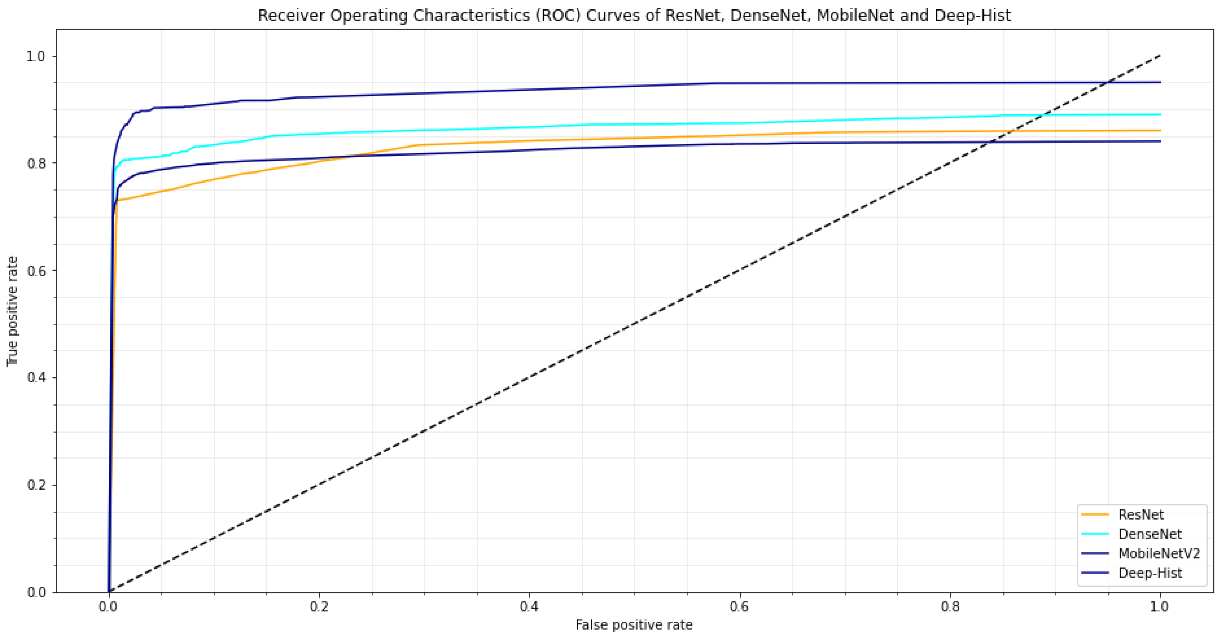
Figure 4, the AUC of the ROC curve is 0.9534 and in Table 4, ResNet had an 87.76 accuracy rate, DenseNet had an 87.59 accuracy rate and MobileNetV2 had an 84.18 accuracy rate. Large and readily available healthcare data sets are used to obtain acceptable categorization outputs. The classification of malignant types is accurate at 95.71%. The plausible outcomes of the proposed framework are evaluated using performance assessment metrics such as ROC curve AUC, precision, specificity, accuracy, and sensitivity.
The use of pretrained Convolutional Neural Network models and our proposed model Deep-Hist to categorize images has lately become popular in the diagnosis of medical analysis. The kind of malignant disease is determined using CNN models in this study. The key hurdle with CNN is figuring out which network architecture is the most successful for a specific situation. Choosing the right hyperparameters is crucial for getting good results, especially with convolutional neural networks. Adaptive Hyperparameter Tuning (AHT) is proposed in this study to construct the most effective CNN framework and to improve the hyperparameters of the CNN models. Large and readily available healthcare data sets such as BreakHis, BraTS, and NIH-Xray are used to obtain plausible classification outputs. The classification of malignant types is accurate at 95.71%. The outcomes of the proposed framework are evaluated using performance assessment metrics such as ROC curve AUC, precision, specificity, accuracy, and sensitivity depicted in Table 4 and Table 5.
It is fascinating to compare the outputs of the proposed CNN model Deep-Hist to those of current dominant advanced CNN models such as ResNet, DenseNet, and MobileNetV2. The same experiment is run with the same combined dataset (COVID-19, BreakHis, NIH-Xray, and BraTS), using well-known pretrained CNNs such as ResNet, DenseNet, and MobileNetV2. Table 4 shows the outcomes of these models. The proposed CNN model Deep-Hist and many common architectures are compared in terms of accuracy and AUC obtained during the experiments. Table 4 and Table 5 shows that the proposed CNN model Deep-Hist outperforms other networks in the classification test. In the task of classification, the DenseNet model, which is close to the proposed CNN model, achieves an accuracy of 87.59%. Pretrained deep learning frameworks for common image classification issues are constructed and learned on generic data sets, which might explain why the proposed CNN models outperform them. On the other hand, the proposed CNN model is designed for a more specific task, namely Breast Cancer classification. In addition, the proposed model Deep-Hist is trained and evaluated using Histopathological images of Breast Cancer, NIH-Xray images of lungs, COVID-19 images of lungs X-ray, and Brain tumors of BraTS. Another factor why the proposed CNN model “Deep-Hist” surpasses the pretrained models is that the proposed CNN architecture was enhanced specifically for the categorization job and used the hyperparameters that generate the optimal results.
Figure 4 also shows that a recall of 0.5 percent denotes that the classification algorithm has a large number of false negatives, which can be caused by imbalanced classes or untuned model hyperparameters, whereas a recall of 1.0 percent demonstrates that the classifier has confidently predicted for the extracted features. Furthermore, when the Area Under the Curve (AUC) is 1 or close to 1, the classification algorithm has successfully discriminated all positive and negative class points, but when AUC is zero, the classification algorithm classified all negatives as positives and vice versa. The True Positive Rate (TPR) is shown against the False Positive Rate (FPR) at varying levels of intensity on the Receiver Operating Characteristics (ROC) Curve. Figure 4 illustrates how classifiers with curves closer to the upper left corner perform better. In addition, when the classifier curve approaches the ROC space’s 45 diagonal, the test becomes less accurate. A probability in the range [0.0, 0.49] implies a negative result (0), whereas a probability in the range [0.5, 1.0] suggests a positive event (1). The Deep-Hist accuracy is 0.95, ResNet = 0.87, MobileNetV2 = 0.84, and DenseNet = 0.88 are closer to the top left corner in the experimental findings.
The two initial hyperparameters which as epochs and kernel/filter values steer the search toward the local maximum on the right side; however, exploration forecasts the algorithm to baffle from that topical optimum and determine the global on the left. We observe how the two hyperparameter point ideas frequently occur in high-uncertainty zones (exploration) and are not just based on the high-degree surrogate function values.
The experimental results and statistical analysis present that while a Random Search (RS) may be effective for a small dataset, it is insufficient for a medium-scale dataset. Due to the intrinsic unpredictability of the acquisition procedure, RS surpasses Grid Search (GS) and Bayesian Optimization (BO) in some circumstances. In comparison, the proposed hyperparameter optimization technique (AHT) is disciplined, with a model-based approach and theoretically sound hyperparameter adjustment. As a result, it is a good choice for large-sized datasets and complicated patterns. The empirical results and statistical analysis further show that the number of hyperparameters to be adjusted, the size of the dataset, and the Imbalance ratio all influence the choice of the HPO method for CNN models. The findings of this study’s trials show that, when compared to Grid Search and Random Search, AHT has the ability to improve classifier demonstration in many circumstances since AHT picks the next hyperparameters with care. As a result, for many of the datasets utilized in this work, it is a superior choice for non-trivial hyperparameter search spaces.
Experiments demonstrate that the Deep-Hist CNN architecture along with the proposed AHT optimization algorithm (Deep-Hist-AHT) may efficiently respond to BreakHis, BraTS, and Covid-19 datasets. Furthermore, the Deep-Hist demonstrates great classification accuracy and F1-Score with acceptable spatial characterization on different pairs of healthcare datasets and outperforms the ResNet, DenseNet, and MobileNetV2 in terms of accuracy, Specificity, Sensitivity, and especially in learnable parameters. The variety in findings shows that simply adjusting the learning rate, activation function and dropout could not be enough to tailor a CNN architecture to different datasets. Furthermore, the collection of optimal hyperparameters we chose for CNN learning framework to adapt and enables the proposed model to suit fresh datasets efficiently. The findings of the Deep-Hist with AHT optimization algorithm and the other pretrained models such as ResNet, DenseNet, and MobileNetV2 with BO approaches indicate that our methodology outperforms the well-known Multi-Objective Bayesian hyperparameter optimization method while delivering significantly smaller structures. Furthermore, it illustrates that using the proposed AHT optimization algorithm to tweak the hyperparameters in the CNN architectures greatly increases the F1-Score, Specificity, and Sensitivity of healthcare datasets.

6. Conclusions

As a response to the rise of deep learning, machine learning research studies have switched from feature engineering to architecture engineering. This work uses CNN models to explain the binary categorization of malignant and benign for the first diagnosis, practically all of which are autonomously adjusted using the Adaptive Hyperparameter Tuning algorithm. A powerful CNN model for identifying malignancy in images is defined using publicly available medical image datasets. The proposed paradigm for classifying medical images into binary classes is 95.71%. The proposed CNN model is trained and assessed on a large enough amount of medical images. The results obtained by the proposed CNN model, as well as comparisons with well-known techniques, demonstrate the CNN model’s utility when developed with the supplied optimization framework. Clinicians and medical practitioners can utilize the CNN model developed in this study to confirm their first screening for malignant and benign binary classification.
The number of repetitions required to estimate the optimized hyperparameters is the suggested AHT optimization algorithm’s shortcoming in comparison to the other proven Bayesian optimization method. Distributed parallelization the learning of potential CNN architectures in each iteration and employing a surrogate-assisted adaptive strategy to decrease the number of architectures taught is workable alternatives to this challenge.
The Deep-Hist model has a fundamental fixed architecture which is a constraint. However, it should be noted that constructing a CNN model entails a large number of optimized hyperparameters that constitute a vast activity effort. To maintain the task numerically and manageably, various hyperparameters must be fine-tuned early. After a complete evaluation of effective CNN models for healthcare image classification, the Deep-Hist constant CNN architecture was established in this study, and it is the strategy that permits the approach to optimize for classification error and model complexity. Furthermore, considering the model’s demonstrated capacity to adjust new healthcare datasets, we feel the unbound collection of hyperparameters offers adequate flexibility.
The approach provided here intends to tackle the prevailing restrictions of adjusting a CNN model to unknown healthcare datasets and user-generated models in medical and clinical situations. In the future, we intend to accelerate the proposed optimization algorithm with other learning frameworks by employing parallel computing methodologies with federated learning and extending the CNN models to dynamically classify and segment 3D/2D healthcare images.

Author Contributions

Conceptualization, S.I.; Methodology, S.I.; Validation, A.N.Q.; Formal analysis, S.I. and J.L.; Investigation, A.N.Q., A.U. and T.M.; Resources, J.L.; Data curation, A.N.Q. and T.M.; Writing—original draft, S.I.; Visualization, A.U.; Supervision, A.N.Q. and T.M.; Project administration, A.N.Q., A.U. and J.L.; Funding acquisition, J.L. All authors have read and agreed to the published version of the manuscript.

Funding

This study is partially supported by the National Key R&D Program of China with the project no. 2020YFB2104402.

Institutional Review Board Statement

Not applicable.

Informed Consent Statement

Not applicable.

Data Availability Statement

Not applicable.

Conflicts of Interest

The authors have no competing interest to declare that are relevant to the content of this article.

References

  1. Ilievski, I.; Akhtar, T.; Feng, J.; Shoemaker, C. Efficient hyperparameter optimization for deep learning algorithms using deterministic rbf surrogates. In Proceedings of the AAAI Conference on Artificial Intelligence, San Francisco, CA, USA, 4–9 February 2017; Volume 31. [Google Scholar]
  2. Ogundokun, R.O.; Misra, S.; Douglas, M.; Damaševičius, R.; Maskeliūnas, R. Medical Internet-of-Things Based Breast Cancer Diagnosis Using Hyperparameter-Optimized Neural Networks. Future Internet 2022, 14, 153. [Google Scholar] [CrossRef]
  3. Bergstra, J.; Bengio, Y. Random search for hyper-parameter optimization. J. Mach. Learn. Res. 2012, 13, 281–305. [Google Scholar]
  4. Bergstra, J.; Bardenet, R.; Bengio, Y.; Kégl, B. Algorithms for hyper-parameter optimization. Adv. Neural Inf. Process. Syst. 2011, 24, 2546–2554. [Google Scholar]
  5. Betrò, B. Bayesian methods in global optimization. J. Glob. Optim. 1991, 1, 1–14. [Google Scholar] [CrossRef]
  6. Jones, D.R. A taxonomy of global optimization methods based on response surfaces. J. Glob. Optim. 2001, 21, 345–383. [Google Scholar] [CrossRef]
  7. Iqbal, S.; Qureshi, A.N. Deep-Hist: Breast cancer diagnosis through histopathological images using convolution neural network. J. Intell. Fuzzy Syst. 2022, 43, 1–18. [Google Scholar] [CrossRef]
  8. Spanhol, F.A.; Oliveira, L.S.; Petitjean, C.; Heutte, L. A dataset for breast cancer histopathological image classification. IEEE Trans. Biomed. Eng. 2015, 63, 1455–1462. [Google Scholar] [CrossRef] [PubMed]
  9. Henry, T.; Carré, A.; Lerousseau, M.; Estienne, T.; Robert, C.; Paragios, N.; Deutsch, E. Brain tumor segmentation with self-ensembled, deeply-supervised 3D U-net neural networks: A BraTS 2020 challenge solution. In Proceedings of the International MICCAI Brainlesion Workshop, Lima, Peru, 4 October 2020; pp. 327–339. [Google Scholar]
  10. Cohen, J.P.; Morrison, P.; Dao, L.; Roth, K.; Duong, T.Q.; Ghassemi, M. COVID-19 Image Data Collection: Prospective Predictions Are the Future. arXiv 2020, arXiv:2006.11988. [Google Scholar]
  11. Jaeger, S.; Karargyris, A.; Candemir, S.; Folio, L.; Siegelman, J.; Callaghan, F.; Xue, Z.; Palaniappan, K.; Singh, R.K.; Antani, S.; et al. Automatic tuberculosis screening using chest radiographs. IEEE Trans. Med. Imaging 2013, 33, 233–245. [Google Scholar] [CrossRef] [PubMed]
  12. Feurer, M.; Eggensperger, K.; Falkner, S.; Lindauer, M.; Hutter, F. Auto-sklearn 2.0: Hands-free automl via meta-learning. arXiv 2020, arXiv:2007.04074. [Google Scholar]
  13. Erickson, N.; Mueller, J.; Shirkov, A.; Zhang, H.; Larroy, P.; Li, M.; Smola, A. AutoGluon-Tabular: Robust and Accurate AutoML for Structured Data. arXiv 2020, arXiv:2003.06505. [Google Scholar]
  14. Liaw, R.; Liang, E.; Nishihara, R.; Moritz, P.; Gonzalez, J.E.; Stoica, I. Tune: A research platform for distributed model selection and training. arXiv 2018, arXiv:1807.05118. [Google Scholar]
  15. Moritz, P.; Nishihara, R.; Wang, S.; Tumanov, A.; Liaw, R.; Liang, E.; Elibol, M.; Yang, Z.; Paul, W.; Jordan, M.I.; et al. Ray: A distributed framework for emerging {AI} applications. In Proceedings of the 13th USENIX Symposium on Operating Systems Design and Implementation (OSDI 18), Carlsbad, CA, USA, 8–10 October 2018; pp. 561–577. [Google Scholar]
  16. Hansen, N. The CMA evolution strategy: A comparing review. In Towards a New Evolutionary Computation; Springer: Berlin/Heidelberg, Germany, 2006; Volume 192, pp. 75–102. [Google Scholar]
  17. Akiba, T.; Sano, S.; Yanase, T.; Ohta, T.; Koyama, M. Optuna: A next-generation hyperparameter optimization framework. In Proceedings of the 25th ACM SIGKDD International Conference on Knowledge Discovery & Data Mining, Anchorage, AK, USA, 4–8 August 2019; pp. 2623–2631. [Google Scholar]
  18. Li, L.; Jamieson, K.; Rostamizadeh, A.; Gonina, E.; Hardt, M.; Recht, B.; Talwalkar, A. Massively Parallel Hyperparameter Tuning. arXiv 2018, arXiv:1810.05934. [Google Scholar]
  19. Jaderberg, M.; Dalibard, V.; Osindero, S.; Czarnecki, W.M.; Donahue, J.; Razavi, A.; Vinyals, O.; Green, T.; Dunning, I.; Simonyan, K.; et al. Population based training of neural networks. arXiv 2017, arXiv:1711.09846. [Google Scholar]
  20. Lindauer, M.; Eggensperger, K.; Feurer, M.; Biedenkapp, A.; Deng, D.; Benjamins, C.; Ruhkopf, T.; Sass, R.; Hutter, F. SMAC3: A Versatile Bayesian Optimization Package for Hyperparameter Optimization. J. Mach. Learn. Res. 2022, 23, 1–9. [Google Scholar]
  21. Falkner, S.; Klein, A.; Hutter, F. BOHB: Robust and efficient hyperparameter optimization at scale. In Proceedings of the International Conference on Machine Learning, Jinan, China, 19–21 May 2018; pp. 1437–1446. [Google Scholar]
  22. Li, L.; Jamieson, K.; DeSalvo, G.; Rostamizadeh, A.; Talwalkar, A. Hyperband: A novel bandit-based approach to hyperparameter optimization. J. Mach. Learn. Res. 2017, 18, 6765–6816. [Google Scholar]
  23. Kandasamy, K.; Vysyaraju, K.R.; Neiswanger, W.; Paria, B.; Collins, C.R.; Schneider, J.; Poczos, B.; Xing, E.P. Tuning Hyperparameters without Grad Students: Scalable and Robust Bayesian Optimisation with Dragonfly. J. Mach. Learn. Res. 2020, 21, 1–27. [Google Scholar]
  24. Li, Y.; Shen, Y.; Jiang, H.; Zhang, W.; Li, J.; Liu, J.; Zhang, C.; Cui, B. Hyper-Tune: Towards Efficient Hyper-parameter Tuning at Scale. arXiv 2022, arXiv:2201.06834. [Google Scholar] [CrossRef]
  25. Balandat, M.; Karrer, B.; Jiang, D.; Daulton, S.; Letham, B.; Wilson, A.G.; Bakshy, E. BoTorch: A framework for efficient Monte-Carlo Bayesian optimization. Adv. Neural Inf. Process. Syst. 2020, 33, 21524–21538. [Google Scholar]
  26. Hutter, F.; Kotthoff, L.; Vanschoren, J. Automated Machine Learning: Methods, Systems, Challenges; Springer: Berlin/Heidelberg, Germany, 2019. [Google Scholar]
  27. Jamieson, K.; Talwalkar, A. Non-stochastic best arm identification and hyperparameter optimization. In Artificial Intelligence and Statistics; PMLR: New York, NY, USA, 2016; pp. 240–248. [Google Scholar]
  28. Domhan, T.; Springenberg, J.T.; Hutter, F. Speeding up automatic hyperparameter optimization of deep neural networks by extrapolation of learning curves. In Proceedings of the Twenty-Fourth International Joint Conference on Artificial Intelligence, Buenos Aires, Argentina, 25–31 July 2015. [Google Scholar]
  29. Klein, A.; Falkner, S.; Springenberg, J.T.; Hutter, F. Learning Curve Prediction with Bayesian Neural Networks. In Proceedings of the 5th International Conference on Learning Representations, ICLR 2017, Toulon, France, 24–26 April 2017. [Google Scholar]
  30. Golovin, D.; Solnik, B.; Moitra, S.; Kochanski, G.; Karro, J.; Sculley, D. Google vizier: A service for black-box optimization. In Proceedings of the 23rd ACM SIGKDD International Conference on Knowledge Discovery and Data Mining, Halifax, NS, Canada, 13–17 August 2017; pp. 1487–1495. [Google Scholar]
  31. Li, Y.; Shen, Y.; Zhang, W.; Chen, Y.; Jiang, H.; Liu, M.; Jiang, J.; Gao, J.; Wu, W.; Yang, Z.; et al. Openbox: A generalized black-box optimization service. In Proceedings of the 27th ACM SIGKDD Conference on Knowledge Discovery & Data Mining, Virtual, 14–18 August 2021; pp. 3209–3219. [Google Scholar] [CrossRef]
  32. Hu, Y.Q.; Yu, Y.; Tu, W.W.; Yang, Q.; Chen, Y.; Dai, W. Multi-fidelity automatic hyper-parameter tuning via transfer series expansion. In Proceedings of the AAAI Conference on Artificial Intelligence, Atlanta, Georgia, 8–12 October 2019; Volume 33, pp. 3846–3853. [Google Scholar]
  33. Li, Y.; Shen, Y.; Jiang, J.; Gao, J.; Zhang, C.; Cui, B. Mfes-hb: Efficient hyperband with multi-fidelity quality measurements. In Proceedings of the AAAI Conference on Artificial Intelligence, Virtual, 2–9 February 2021; Volume 35, pp. 8491–8500. [Google Scholar] [CrossRef]
  34. Kandasamy, K.; Krishnamurthy, A.; Schneider, J.; Póczos, B. Asynchronous Parallel Bayesian Optimisation via Thompson Sampling. Stat 2017, 1050, 25. [Google Scholar]
  35. González, J.; Dai, Z.; Hennig, P.; Lawrence, N. Batch Bayesian optimization via local penalization. In Proceedings of the Artificial Intelligence and Statistics, 19th International Conference on Artificial Intelligence and Statistics (AISTATS) 2016, Cadiz, Spain, 9–11 May 2016; Volume 41, pp. 648–657. [Google Scholar]
  36. Alvi, A.; Ru, B.; Calliess, J.P.; Roberts, S.; Osborne, M.A. Asynchronous Batch Bayesian Optimisation with Improved Local Penalisation. In Proceedings of the International Conference on Machine Learning, Long Beach, CA, USA, 9–15 June 2019; pp. 253–262. [Google Scholar]
  37. Klein, A.; Tiao, L.C.C.; Lienart, T.; Archambeau, C.; Seeger, M. Model-based Asynchronous Hyperparameter and Neural Architecture Search. arXiv 2020, arXiv:2003.10865. [Google Scholar]
  38. Siems, J.; Zimmer, L.; Zela, A.; Lukasik, J.; Keuper, M.; Hutter, F. NAS-Bench-301 and the Case for Surrogate Benchmarks for Neural Architecture Search. arXiv 2020, arXiv:2008.09777. [Google Scholar]
  39. Ma, L.; Cui, J.; Yang, B. Deep Neural Architecture Search with Deep Graph Bayesian Optimization. In Proceedings of the IEEE/WIC/ACM International Conference on Web Intelligence, Thessaloniki, Greece, 14–17 October 2019; pp. 500–507. [Google Scholar]
  40. Kandasamy, K.; Neiswanger, W.; Schneider, J.; Poczos, B.; Xing, E.P. Neural architecture search with bayesian optimisation and optimal transport. Adv. Neural Inf. Process. Syst. 2018, 31, 2020–2029. [Google Scholar]
  41. Real, E.; Aggarwal, A.; Huang, Y.; Le, Q.V. Regularized evolution for image classifier architecture search. In Proceedings of the AAAI Conference on Artificial Intelligence, Honolulu, HI, USA, 27 January–1 February 2019; Volume 33, pp. 4780–4789. [Google Scholar] [CrossRef] [Green Version]
  42. Xu, Y.; Xie, L.; Zhang, X.; Chen, X.; Qi, G.J.; Tian, Q.; Xiong, H. PC-DARTS: Partial Channel Connections for Memory-Efficient Architecture Search. In Proceedings of the International Conference on Learning Representations, New Orleans, LA, USA, 6–9 May 2019. [Google Scholar]
  43. Snoek, J.; Larochelle, H.; Adams, R.P. Practical bayesian optimization of machine learning algorithms. Adv. Neural Inf. Process. Syst. 2012, 25, 2951–2959. [Google Scholar]
  44. Olson, R.S.; Moore, J.H. TPOT: A tree-based pipeline optimization tool for automating machine learning. In Proceedings of the Workshop on Automatic Machine Learning, New York, NY, USA, 24 June 2016; pp. 66–74. [Google Scholar]
  45. Dong, X.; Yang, Y. NAS-Bench-201: Extending the Scope of Reproducible Neural Architecture Search. In Proceedings of the International Conference on Learning Representations, New Orleans, LA, USA, 6–9 May 2019. [Google Scholar]
  46. Atteia, G.; Abdel Samee, N.; El-Kenawy, E.S.M.; Ibrahim, A. CNN-Hyperparameter Optimization for Diabetic Maculopathy Diagnosis in Optical Coherence Tomography and Fundus Retinography. Mathematics 2022, 10, 3274. [Google Scholar] [CrossRef]
  47. Vrbačič, G.; Pečnik, Š.; Podgorelec, V. Hyper-parameter optimization of convolutional neural networks for classifying COVID-19 X-ray images. Comput. Sci. Inf. Syst. 2022, 19, 327–352. [Google Scholar] [CrossRef]
  48. Aytaç, U.C.; Güneş, A.; Ajlouni, N. A novel adaptive momentum method for medical image classification using convolutional neural network. BMC Med. Imaging 2022, 22, 1–12. [Google Scholar] [CrossRef] [PubMed]
  49. Atteia, G.; Alhussan, A.A.; Samee, N.A. BO-ALLCNN: Bayesian-Based Optimized CNN for Acute Lymphoblastic Leukemia Detection in Microscopic Blood Smear Images. Sensors 2022, 22, 5520. [Google Scholar] [CrossRef] [PubMed]
Figure 1. Intuited Filter: Getting filter and optimized hyperparameters from Bayesian optimization with Tree Parzen Estimator (TPE) Estimator.
Applsci 12 11870 g001
Figure 2. Proposed a novel Hybrid approach for acquiring intelligently and optimized hyperparameters (AHT): We have passed a sample of the combined dataset to our proposed black box model with lists of hyperparameters to process with both Gaussian Process (GP) and Tree Parzen Estimator (TPE) and then the optimal value will send to Probability Improvement (PI) and Expected Improvement (EI) to obtain the next sample value.
Applsci 12 11870 g002
Figure 3. The iteration of the combined dataset to acquire optimal results using various hyperparameters such as learning rate (depicted in the first row), batch size (presented in the middle row), and activation function (shown in the last row) and its values.
Applsci 12 11870 g003
Figure 4. Our proposed CNN model (Deep-Hist) is compared with pretrained models like as ResNet, DenseNet and MobileNetV2 on combined dataset (images acquired and combined from BreakHis, COVID-19 X-ray, NIX X-ray and BraTS). The acquired accuracy of pretrained models are ResNet (0.87), DenseNet (0.88) and MobileNetV2 (0.84).
Applsci 12 11870 g004
Table 1. Kernel Value vs. Learning Rate for Binary Classification: CNN model “Deep-Hist” for training with hyperparameter optimization using the proposed algorithm (AHT) and achieved plausible results with a kernel value of 3 and a learning rate of 0.0001.
Learning Rate
0.010.0010.00010.00001
30.87/13.80.88/13.60.95/13.30.86/14.1
Kernel50.83/15.30.86/14.90.84/15.70.88/15.9
70.86/17.50.84/17.70.87/17.30.85/18.2
90.81/18.50.82/18.10.80/18.40.83/17.8
Table 2. Kernel Value vs. Batch Size for Binary Classification: CNN model “Deep-Hist” for training with hyperparameters such as Batch Size and Kernel Values optimization using the proposed algorithm (AHT) and achieved plausible results with a Batch Size of 32 and Kernel Value as 3.
Batch Size
8163264
30.88/13.60.86/13.40.95/13.30.89/13.7
Kernel50.86/15.30.82/14.90.88/15.90.86/15.7
70.86/17.50.84/17.70.87/17.30.85/18.2
90.82/18.10.81/18.50.83/17.80.80/18.4
Table 3. Kernel Value vs. Activation Functions (AF) for Binary Classification: CNN model “Deep-Hist” for training with hyperparameters such as Activation Functions (relu, leakyRelu, swish, mish) and Kernel Values optimization using the proposed algorithm (AHT) and achieved plausible results with activation function as swish and Kernel Value as 3.
Activation Function
reluleakyreluswishmish
30.89/12.90.87/13.20.95/12.70.90/13.4
Kernel50.87/15.70.85/14.60.89/14.30.87/14.3
70.88/17.30.83/17.50.88/26.70.87/16.9
90.85/18.30.83/18.10.85/27.30.83/17.5
Table 4. Training output of Accuracy, F1-Score, Specificity, Precision and Sensitivity on combine datasets.
ModelSensitivitySpecificityPrecisionAccuracyF1-ScoreTrainable Parameter
ResNet83.4384.5787.1787.2686.39>58.5 M
DenseNet86.7986.9787.9387.5988.74>12.8 M
MobileNetV284.9785.1384.5784.1885.13>0.44 M
Deep-Hist93.1193.5194.7195.7193.57<0.27M
Table 5. Training Accuracy, F1-Score, Specificity, Precision and Sensitivity on different datasets such as BraTS, BreakHis, NIH X-ray.
DatasetModelSensitivitySpecificityPrecisionAccuracyF1-Score
BraTSResNet79.1379.6680.2380.3579.84
DenseNet80.1980.3580.7680.5980.74
MobileNetV281.2280.3280.7480.2581.41
Deep-Hist91.3890.4290.4991.0890.84
BreakHisResNet78.2978.7179.0679.0179.15
DenseNet79.6580.0580.1280.2479.85
MobileNetV280.2780.9180.6380.2781.07
Deep-Hist90.3791.1491.0991.2691.37
NIH X-rayResNet82.1182.6782.9682.7883.02
DenseNet84.3684.0184.3684.2584.39
MobileNetV283.8982.8583.7483.9784.08
Deep-Hist92.2892.7192.6993.2192.83
Publisher’s Note: MDPI stays neutral with regard to jurisdictional claims in published maps and institutional affiliations.

