
Adaptive Dynamic Search for Multi-Task Learning


School of Computer Science and Engineering, Chung-Ang University, Seoul 06974, Republic of Korea
Appl. Sci. 2022, 12(22), 11836; https://doi.org/10.3390/app122211836
Submission received: 23 September 2022
/
Revised: 17 November 2022
/
Accepted: 17 November 2022
/
Published: 21 November 2022
(This article belongs to the Topic Machine and Deep Learning)
Abstract
:Multi-task learning (MTL) is a learning strategy for solving multiple tasks simultaneously while exploiting commonalities and differences between tasks for improved learning efficiency and prediction performance. Despite its potential, there remain several major challenges to be addressed. First of all, the task performance degrades when the number of tasks to solve increases or the tasks are less related. In addition, finding the prediction model for each task is typically laborious and can be suboptimal. This nature of manually designing the architecture further aggravates the problem when it comes to solving multiple tasks under different computational budgets. In this work, we propose a novel MTL approach to address these issues. The proposed method learns to search in a finely modularized base network dynamically and to discover an optimal prediction model for each instance of a task on the fly while taking the computational costs of the discovered models into account. We evaluate our learning framework on a diverse set of MTL scenarios comprising standard benchmark datasets. We achieve significant improvements in performance for all tested cases compared with existing MTL alternatives.
1. Introduction
Undoubtedly, deep learning has been a popular choice of learning strategies in many fields of study [1] and has achieved remarkable success in solving challenging problems in computer vision and machine learning [2,3,4,5,6]. To that end, it became a general trend for practitioners to develop a neural network model specifically tailored for a given task to improve the performance [4,6,7]. With high memory requirements for an increasing number of tasks as well as manual efforts in designing the architectures, however, this approach (i.e., one network for a single task) is often found to be non-scalable and presents challenges to be employed for multifunctional devices with limited resources [8].
To address this issue, multiple tasks are learned simultaneously via a shared network architecture in a multi-task learning regime (MTL) [9,10]. MTL is a learning strategy for solving multiple tasks at the same time while exploiting commonalities and differences across tasks. This learning strategy turned out to be effective for diverse applications [3,11,12,13,14,15,16]. Nonetheless, there remain several challenges that need addressing. First, the performance can degrade when the number of tasks to be learned is high or the tasks are not closely related [17,18]. Second, manually designing novel architectures for MTL is challenging due to the difficulty of curating optimal prediction models. Last but not least, a naïve MTL approach entails highly demanding efforts when cost-adaptivity is required (i.e., performing tasks adaptively for different computational and memory costs). This also requires searching for the corresponding network models manually. Despite the practical benefit of tackling it, this combinatory problem has not been addressed rigorously as of yet.
In this work, we propose a novel MTL approach that is cost-adaptive and enables dynamic model search. Given a computation budget, our approach produces a network suited for each task automatically (without the need to design the architecture) on the fly and instance-wise (i.e., a network for an instance). The proposed approach provides a wide range of solutions with respect to different computational budgets for each task, as shown in Figure 1. This is achieved by exploring multiple network models automatically (without the need to manually design the architecture) on the fly and instance-wise in a single learning procedure. To this end, we develop a unified framework that consists of two major components, namely backbone and search networks. The backbone network provides a pool of candidate models of different sizes and configurations, from which the search network selects a set of models of different sizes that is most suitable for a given instance with different computational requirements. To offer diverse choices of candidate models, we finely modularize the backbone architecture that constitutes the basic building blocks of disjointed collections of parameters. Then, we construct a new modularized residual block containing the basic building blocks to enrich the search space for competitive dynamic search. The proposed framework is trained for the task performance as well as the computational cost using stochastic gradient descent in an alternating manner. The overall framework of the proposed approach is illustrated in Figure 2. Once the training is complete, the search network can discover different models of choice trading off between the performance and the computational cost for each instance of a task. This can save a significant amount of time and effort in training models of different costs individually.
We evaluate the proposed approach for a range of multi-task learning scenarios using the standard image classification datasets. The experimental results show that the proposed dynamic search method not only achieves higher classification accuracy in the target tasks compared with other existing MTL approaches with a notable performance margin but also provides cost-adaptive solutions. Interestingly, the proposed method can address task difficulty (i.e., searching models with low and high computation costs for easy and hard tasks, respectively) and implicitly group similar instances across tasks (datasets). We further provide comprehensive analyses to validate the effectiveness of the proposed approach. The contributions of this work are mainly fourfold:
- We propose a novel MTL approach that simultaneously solves the problem of interference among instances, manual design efforts, and cost-adaptive search.
- Our cost-adaptive search enables producing multiple models of different costs in a single shot rather than learning a single model of a cost at a time.
- We present a new modularized residual block to enrich the search space and encourage discovering high-performance models.
- The experimental results show the superiority of the proposed method compared to existing strong MTL approaches for a diverse set of MTL scenarios.
This paper is organized as follows. In Section 2, we briefly review the related works on multi-task learning, resource-efficient learning, and dynamic model search. The proposed method for discovering multiple models by dynamic model search is described in Section 3. In Section 4, we present various experimental results on several benchmark datasets to demonstrate the efficiency and competitiveness of the proposed method.
2. Related Work
2.1. Multi-Task Learning
Multi-task learning (MTL) is a learning strategy for solving multiple tasks at the same time while exploiting commonalities and differences across tasks. Compared with training models separately for each task, MTL can improve the learning efficiency as well as the performance of individual tasks [9]. The fundamental idea is to utilize the inductive bias contained in related tasks via a shared representation, which is essentially accomplished by sharing parameters [10] either with a single shared network [13,19] or multiple networks with soft parameter sharing [11,20]. Naturally, many MTL approaches have capitalized on learning inherent commonalities among tasks via architectural variations [11,21]. If tasks are less related, however, these approaches can degrade due to the negative interference arising between the tasks [17,18]. Notably, the performance can degrade further when the samples within a task are of limited relevance. On the contrary, our method explicitly learns for each sample in a task in an instance-wise manner and dynamically generates an optimal network without the need to manually modify the architecture, resulting in a significant increase in performance.
2.2. Resource-Efficient Learning
In this work, we focus on memory-efficient MTL by performing multiple tasks within a single shared architecture without introducing many parameters. Several recent works constructed a k-in-1 type network architecture to provide adaptive solutions for different computational requirements [8,13,22,23,24]. Essentially, they address MTL by executing a different part of a model and save memory footprints that arise in the opposite case of using multiple task-specific models. Recently, the authors of [25] proposed solving MTL with respect to different memory budgets while offering a range of solutions from a single model. Our approach complements their work by addressing the potential suboptimality in their hand-crafted framework via dynamic model search.
2.3. Dynamic Model Search
In recent years, there has been a surge in automating the design of neural network architectures [14,15,16,17,18,26,27,28,29,30]. In this paradigm of automatic model search, the search method dynamically discovers an optimal configuration of a network structure given a base architecture containing multiple choices of building blocks [17,28,29,30,31] or a set of hyperparameters to choose from [26,32]. While avoiding the effort of manual design, this approach can improve the performance over conventional hand-designed network models with the same model capacity [4,33]. Our work is closely related to a few recent works that performed automated model search for MTL [17,31,34]. Notably, however, they were not capable of executing a cost-adaptive search with respect to different computational costs from their learned models, whereas our method produces a range of different solutions with respect to tasks and computation budgets. What is more, the proposed method produces a bespoke solution for each instance, potentially avoiding interference among instances across tasks.
2.4. Contributions
The main contribution of this work is in the development of a dynamic, cost-adaptive search procedure that can solve multi-task learning (MTL) problems effectively within a single training phase. Our cost-adaptive search enables producing multiple models of different costs in a single shot rather than resulting in a single model of a cost at a time, which to our best knowledge has not been addressed in existing works in the MTL literature. This can provide various choices of models trading off between the model performance and cost so that one can save a significant amount of time and effort in training different models for different budgets while solving multiple tasks simultaneously. We highlight the important features of each of the dynamic search approaches in Table 1.
3. The Proposed Method
The proposed multi-task learning framework consists of two major components: a backbone network and a search network. In essence, the backbone network is a large base network that is modularized and serves a search space in which the search network explores to choose the final prediction model (Section 3.1). The search network is designed to select multiple models of different computational costs from the backbone network for each instance of a task (Section 3.2). The entire framework is trained from end to end using the standard gradient descent as well as a policy gradient methods, with the objective of maximizing the performance of different models of sizes selected from the backbone network while regularizing the computational costs of them (Section 3.3). After training, our framework produces a diverse set of prediction models all at once for a given instance of a task. The overall framework and workflow are illustrated in Figure 2.
3.1. Backbone: Modularization for Diverse Models
We constructed a backbone network based on the popular residual network [4,36]. The basic residual block (ResBlock) in the residual network has two convolution layers of weight tensors, and we split each convolution layer of the ResBlock into g groups to modularize the weight tensors. Specifically, let and be the weight tensors corresponding to the two layers in the ResBlock, where w, h, , and are the width, height, and the number of input and output channels, respectively. Then, the modularized residual block, which we term ResBlock-M, contains g channel groups in each layer with their corresponding weight tensors , , …, , , , …, , where
Note that the ith weights and are associated with the ith groups in two layers in ResBlock-M. Rather than utilizing convolutional channels in each layer as a single group, as deep learning methods generally apply [4,6], we treated them in a finer way for searches. Based on the modularization, we constructed the ith building block as two consecutive ith groups in ResBlock-M (see Figure 3). The building blocks can then be chosen by the search network to construct the final prediction model to perform a task.
By using the building blocks, we define the operation in the modularized residual block. In the conventional residual block (ResBlock), we have the following operation:
where is an input for the block and is a function consisting of two layers with and . If does not match with , then we bridge the gap by applying zero padding or a 1 × 1 convolution. In ResBlock-M, we have g functions according to the number of groups (i.e., ), where contains the ith building block. The operation of the proposed residual block becomes
where determines whether to use the function . Notice that the operation in Equation (2) is order-invariant for the functions (or their associated groups). This enriches the search space by providing more diverse choices for the network model compared with module-based approaches which, in general, have g compositions [8,37], and the number of possible compositions increases to . Therefore, the chance of finding a better model increases with the larger, finely modularized search space under the same baseline model.
3.2. Dynamic Model Search
The search network discovers multiple model structures instance-wise dynamically by exploring a collection of candidate models in the backbone. For now, we assume that we are searching for a single model for each instance. Suppose that the backbone network has r ResBlock-M, each of which has g building blocks. The search network can select nothing (equivalent to layer skipping) for all of the building blocks, providing candidate models (search space) in the backbone. Given an input instance x, the search network (The model structure, which is simple, is described in Section 4.2) outputs the probability distribution over compositions of g building blocks in each ResBlock-M. To produce a model, the output of the search network is obtained as follows:
where denotes the set of parameters in the search network. Each column of reveals the probabilities of selecting building blocks over candidates in a ResBlock-M (i.e., ). Here, is the number of elements in the power set of a residual block containing g building blocks. From , we collect a model structure :
Here, or indicates whether to select the ith composition of the building blocks in the j-th ResBlock-M or not, respectively. The probability of a candidate model for an instance x is computed as follows:
where ⊙ is the element-wise multiplication operator. One of candidate models is chosen by the search network when an instance x is given.
In the proposed method, the search network enables an instance-wise search by discovering a suitable model for each instance of a task, rather than searching for a single model for each task [17,26,29,30]. This will prevent potential destructive interference not only between tasks but also within tasks. Our method can provide an on-the-fly bespoke solution tailored to each sample.
In order to perform cost-adaptive predictions for different computational requirements on a per sample basis, the search network explores models for the costs in a single learning procedure. The discovered models will have trade-offs between task accuracy and resource usage (e.g., the number of parameters and FLOPs). This is achieved by simply introducing multiple model structures and learning multiple regularizers accordingly for the computational costs as described in the following section. This approach could be more efficient than other model search methods [17,29], as they choose a single model of a trade-off at a time (i.e., one individually trained model for a cost). If another computational cost is required for a device, then the existing methods need to be retrained to explore another trade-off for the budget.
In addition, we learned a single search network to discover models with respect to the tasks and computational costs, which is universal, unlike introducing multiple search networks (i.e., one search network for a task or a cost). This strategy can naturally supervise all associated tasks at the same time and learn task relationships, producing solutions tailored for each task (see Section 4.3).
3.3. Optimization
Suppose that a set from dataset consists of data instances from different tasks and their task numbers (i.e., ), where and are the data instance and its label, respectively, from the tth dataset . The proposed method optimizes the expected loss to learn two sets of parameters, and , for the backbone architecture and the search network, respectively. We define the objective function that contains the loss functions of the selected models with regularization for all instances as follows:
where , denotes a loss function, f denotes the selected model, c is the number of different computational budgets, and is the model structure for the lth budget selected by the search network by optimizing the following regularization:
Here, denotes the number of parameters specified by in the jth ResBlock-M, denotes the total number of parameters in the jth ResBlock-M, and is the lth weighting factor. By optimizing c different regularizations, the search network is taught to generate c models (, l = 1, 2, …, c) of different computational budgets.
In order to optimize Equation (6) with respect to and , we introduce an alternating optimization strategy which alternatively learns to optimize the models’ losses and the regularizer and learns a set of parameters in corresponding to the generated models to improve their task performance. We optimize the parameters in specified by the selected model structures from ) for each instance using a standard gradient descent method. To learn the set of parameters , we adopt a common approximation strategy in policy gradient methods [38] due to the difficulty of computing the exact expected value in Equation (6) with respect to . Suppose that is the objective function with respect to . By using the log derivative trick on the expected loss with the probability in Equation (5), we approximate the gradient of as follows:
where . The last relation approximates the computation of all possible models in the search space using a set of model structures randomly sampled from [39]. This learning approach resembles a single-step Markov decision process (MDP) by predicting all actions at once via based on a reward [28]. In addition, we apply the epsilon-greedy method [40] on the output when approximating the gradient to allow for a more dynamic search of the network models.
The proposed method, which we named ADM, is summarized in Algorithm 1. In the algorithm, we adopt an alternating optimization approach to learn the sets of parameters and , where we update each set of parameters until convergence in every learning step. We update the parameters in with respect to the discovered network model for each instance. After finishing the learning procedure, we have a trained backbone architecture containing a pool of candidate models and a trained global search network that has knowledge of multiple tasks.
| Algorithm 1 ADM: Adaptive Dynamic Search for MTL |
4. Experiments
The proposed method, which we named ADM for Adpative Dynamic search for Multi-task learning, was evaluated over a range of multi-task learning problems. In the following subsections, we describe the experimental set-up, the implementation details of the proposed method, and the results for four scenarios.
4.1. Set-Up
Each task involved the problem of performing image classification, comprising one of the following standard benchmark datasets: CIFAR-10 and CIFAR-100 [41], Tiny-ImageNet (https://www.kaggle.com/competitions/tiny-imagenet/data, accessed on 22 September 2022), STL-10 [42], or Mini-ImageNet [43]. We further employed CIFAR-MTL [17], the multi-task version of CIFAR-100 that contains 20 superclasses, and each superclass has 5 subclasses, for which we treated each superclass as a task. For Mini-ImageNet, we followed the practice in [17], wherein we randomly chose 50 classes and created 10 tasks of 5 different classes from the chosen classes. We generated 10 different sets of 50 classes and reported the averaged results.
In this work, we consider the four following scenarios:
- Scenario 1: The first scenario is learning two tasks from two datasets of the same domain, CIFAR-10 and CIFAR-100, where each dataset corresponds to a task.
- Scenario 2: The second scenario is a three-task learning problem comprising three datasets (CIFAR-100, Tiny-ImageNet, and STL-10), where each task characterizes different image scales and the number of classes.
- Scenarios 3 and 4: Following a previous work [17] (model selection for MTL), we use the CIFAR-MTL and Mini-ImageNet datasets as other scenarios which are 20-task and 10-task learning problems, respectively.
Table 2 shows the summary of the scenarios.
We compare ADM with strong MTL alternatives: the cross-stitch network [11], routing network [17], PackNet [13], NestedNet [8], and VirtualNet [25]. Among them, VirtualNet and ADM are able to perform cost-adaptive predictions which can produce a larger number of solutions for different computational costs than the other compared methods. The results for PackNet, NestedNet, and VirtualNet were taken from [25] for the first two scenarios. Additionally, the results for the cross-stitch network and routing network were taken from [17] for CIFAR-MTL and Mini-ImageNet. For all experiments, we used the same network architectures as the ones used in the compared methods for fair comparisons.
4.2. Implementation Details
We used three convolutional neural networks from small-scale to large-scale in this work: a simple convolutional network [17], (Since it does not have residual connections, the search space for the backbone architecture becomes .) residual network [4], and wide residual network [36]. When we applied the residual networks for the first and second scenarios, we constructed architectures suitable for the CIFAR and ImageNet datasets, respectively. The fully connected layers in the backbone networks were not modularized to groups. The search network consisted of three conventional residual blocks (six convolutional layers) and one fully connected layer for Scenarios 1 and 2, and it consisted of four convolutional layers and one fully connected layer for Scenarios 3 and 4. Note that the size of the search network was smaller than the backbone, and the memory increment was marginal.
The backbone network was pretrained before we started to optimize the framework. During pretraining, we randomly dropped some building blocks, similar in spirit to [44]. While it resembled our procedure of dynamic search, we found that this strategy improved the overall performance, even though we fine-tuned the parameters in the backbone in the alternating optimization procedure. All compared methods were initialized with Xavier initialization [45] and trained using the Nesterov Accelerated Gradient optimizer [46] with a momentum decay of 0.9, following the standard set-up. For the search network, we used the Adam optimizer [47]. When learning the parameters of the selected models, we applied the standard weight decay. We used batch sizes of 128 and 64 for the first and second scenarios, respectively, where the initial learning rate was 0.1 and decreased by 10 when converging, while the batch size was 256 for the rest of the scenarios, where the initial learning rate was 0.01 and reduced by 10. We applied different values to construct models of different computational budgets.
4.3. Results
4.3.1. Scenario 1
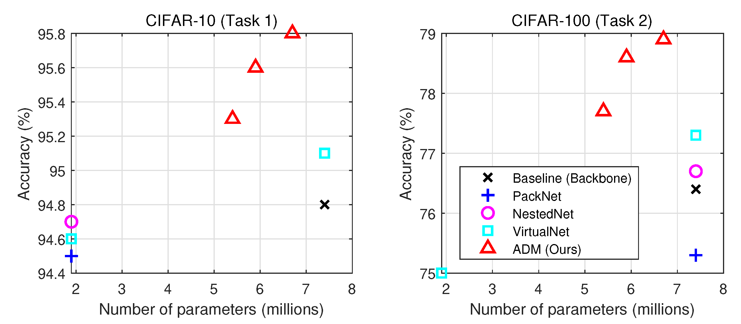
We first applied the proposed method, ADM, to the first scenario and compared it with several recent approaches that can perform multiple tasks: NestedNet, PackNet, (A modified version of PackNet was applied as in [25]) and VirtualNet, including a multi-task learning baseline method. While NestdNet and PackNet produce outputs corresponding to tasks under different computational budgets (number of parameters), VirtualNet and ADM can produce a larger number of outputs for tasks and budgets. Note that the number of outputs (models) with respect to computational budgets in VirtualNet should be the same as the number of tasks [25], which limits its applicability, whereas ADM allows the search network to choose the number of different computational budgets regardless of the number of tasks. (Here, the number of computational budgets c is set to three.) We used WRN-32-4 [36] for all compared approaches, whose total number of parameters was 7.4 million.
Figure 4 shows the experimental results, where ours give the average of the individual results of all instances for each task. At first, the solutions obtained by ADM improved over the baseline while using a lower number of parameters for both tasks. Overall, ADM produces three outputs of different computational budgets, and all of them outperformed other methods being compared while consuming lower computational budgets. Since the proposed approach performed adaptive dynamic search for each instance, it could produce a bespoke model and the solution for each instance rather than giving a single hand-crafted model for a task. Aside from that, it automatically selected an optimal structure, enabling performance improvement compared with other competitors that are based on a fixed manual model structure. Notice that the models explored by the search network were distributed in a region (5.3–6.7 million) in the computational budget. This is potentially because the probability of choosing the compositions of the intermediate number of building blocks was dominant among possible compositions using g building blocks, whereas the probability of choosing extreme cases (i.e., compositions with few or most of the building blocks chosen) was scarce when optimizing the loss function (Equation (6)).
4.3.2. Scenario 2
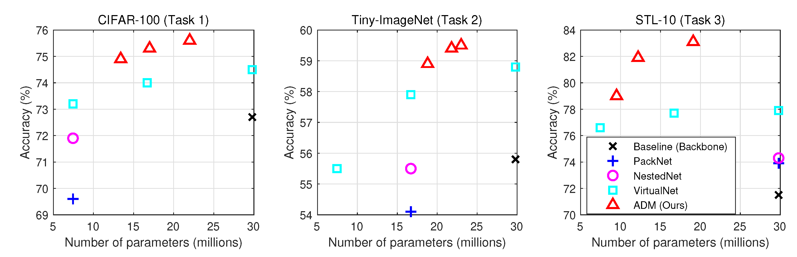
Then, we evaluated ADM for the second scenario, where there were three tasks of different input scales to solve. This scenario was more difficult to solve than the previous one because the associated tasks contained different distributions and domains. To solve this problem, we introduced task-specific input layers for all compared methods that were the same as those in the previous scenario. Similar to the previous experiment, NestedNet and PackNet produced three outputs of different computational budgets for the tasks, and VirtualNet and ADM produced nine different solutions with respect to the tasks and budgets. Following the practice in [25], all methods were compared based on the ResNet-42 architecture, whose number of parameters was 28.2 million.
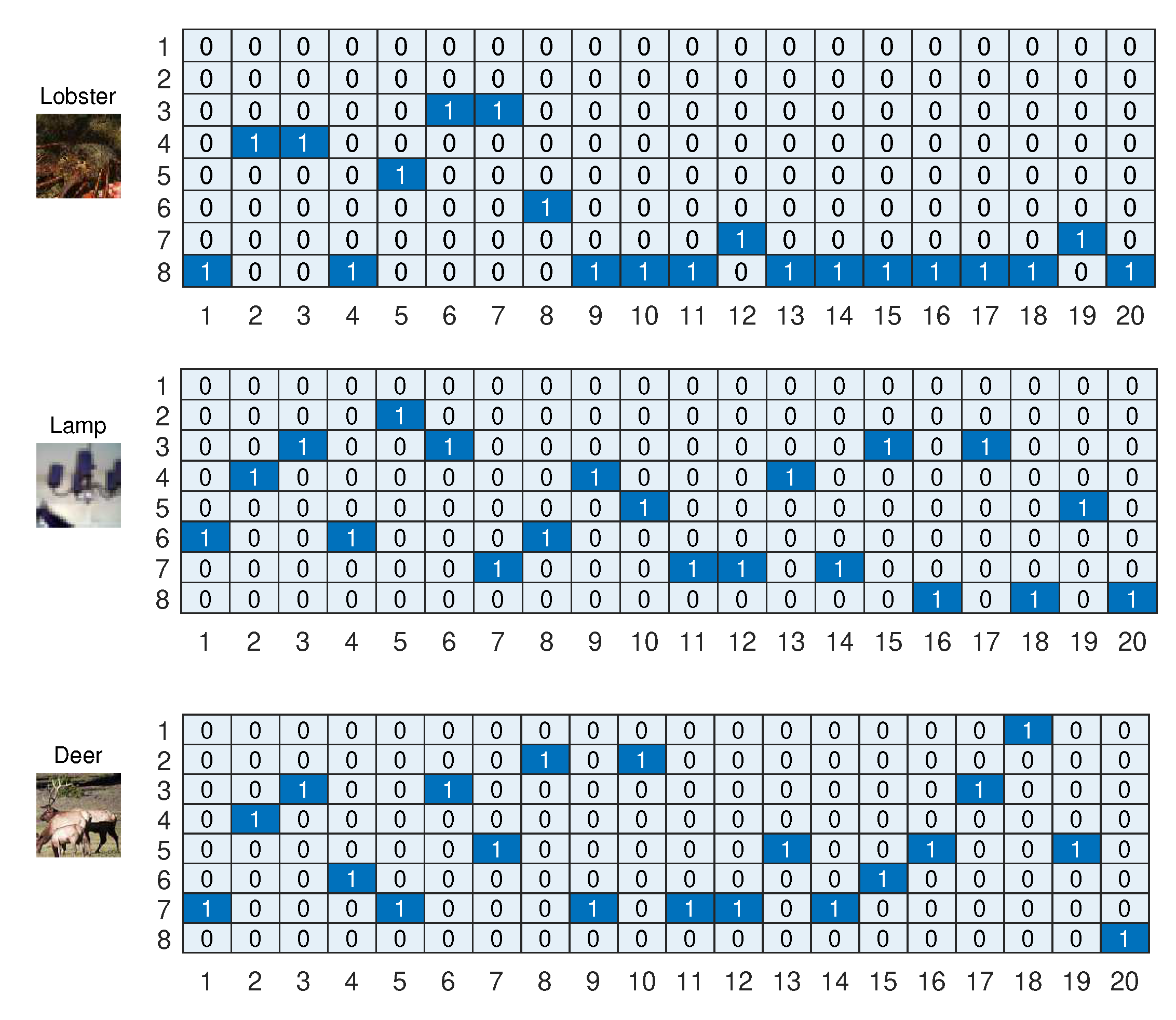
The performance comparison is shown in Figure 5. Similar to the previous result, ADM achieved excellence performance compared with the other methods. The baseline performed much worse than ours while requiring a larger number of parameters (e.g., for Task 3, from 1.5× to 3× larger number of parameters). ADM also performed better than VirtualNet under a similar budget which could produce varying solutions of different costs (e.g., for Task 3, 9–19 million parameters). From the figure, we can observe that the performance improvement was notable for STL-10 when comparing the models of the highest cost (i.e., from 4% to 11% higher accuracy than other methods while taking a reduced budget of around 35%). It is interesting to note that the search network automatically explored a wider range of models with lower cost requirements when the number of classes was lower (i.e., easier). In other words, the search network chose models of a lower number of parameters for Task 3, the easier task (10 classes, 10–18 million), than the harder tasks of Task 1 (100 classes, 13–22 million) and Task 2 (200 classes, 18–23 million). This tendency indicates the benefit of the single universal search network learning the comprehensive knowledge from all the tasks. Figure 6 gives the selected models for three different images. The search network automatically discovers a cost-intensive model for an indistinguishable image (top) and a model of a low-cost requirement for a clearly discriminating image (bottom).
4.3.3. Scenario 3
In order to see how ADM compared against other methods when there was a larger number of tasks to solve, we evaluated ADM on CIFAR-MTL. Recall that this is a 20-task learning problem. We compared them with a cross-stitch network and routing network, which can perform such tasks. Note that it is difficult for NestedNet, PackNet, and VirtualNet to train a large number of tasks within a single architecture because the size of assigned parameters for each task will be reduced too much as the number of tasks increases. They are trained for less than five tasks and hence are limited in learning capacity for scenarios where there are many tasks to learn and solve. We employed the same architecture used in the routing network [17] for comparison. The architecture consisted of four convolutional layers without the residual connection and three fully connected layers occupying 74,000 parameters. The search network in ADM produced two models of different parameter budgets in this scenario.
The experimental results of the scenario are summarized in Table 3, where we compare the approaches for classification accuracy (i.e., average accuracy for all tasks) and the number of parameters used in the applied network. The experiment also shows the excellence of the proposed method for many tasks compared with the multi-task learning baseline and other methods. Specifically, the proposed method performed better than the routing network, the major competitor based on model selection giving the highest accuracy among the competitors, by a margin of 4.5–6.6% under the reduced number of parameters (around 25–50% parameters). Note that the cross-stitch network and routing network generally allowed larger memory than the baseline due to their stitching and routing mechanisms. That aside, the compared methods did not produce a set of distributed solutions as ours did in a trained framework. This scenario also shows the benefit of the proposed method for many tasks.
4.3.4. Scenario 4
To further compare the proposed method with the competitors of the previous scenario in a large number of tasks, we followed the experiment in [17] using Mini-ImageNet (10-task learning). We compared the same approaches to the previous scenario under the architecture applied in [17], which occupied 140,000 parameters. The proposed method produced two network models of different parameter budgets, which are 60,000 and 110,000, respectively, from the search network.
Table 4 shows the performance comparison of the compared approaches. Notably, ADM outperformed other methods by a larger margin than the previous experiment (i.e., 14.5–22.5% higher accuracy). Aside from that, the proposed method required fewer parameters than the compared approaches (43–80% reduced parameters). While the routing network, a strong competitor, performed better than the baseline and the popular cross-stitch network as it consumed a similar number of parameters, it performed much poorer than the proposed method while occupying a larger number of parameters. The adaptive dynamic search under the rich search space in ADM allows the chance to discover an optimized model and the solution for each instance, which therefore delivers such remarkable performance improvement compared with other alternatives.
4.4. Analysis
4.4.1. Qualitative Analysis
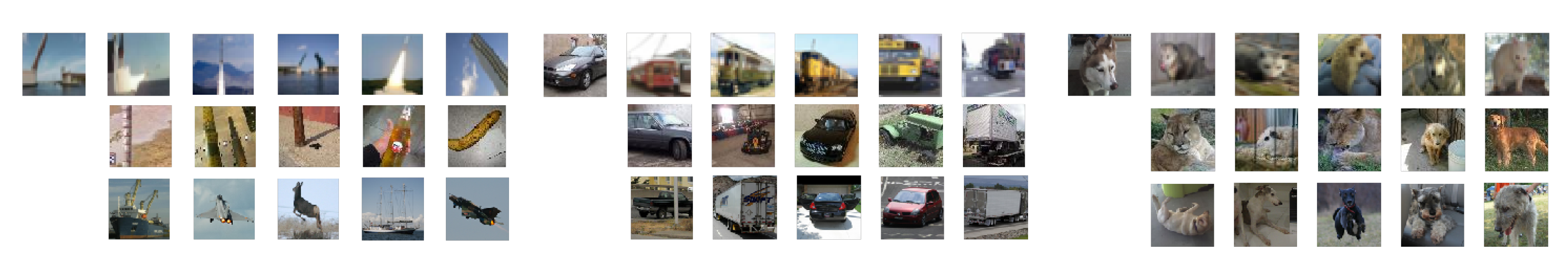
One of the features of the proposed method is that it learns multiple tasks in an instance-wise fashion. Figure 7 provides similar images given a query image from each task. The similar images had their model structures explored by the search network, which were similar to that of the query image. One interesting aspect is that for the first query image (“rocket”), the similar images (“birds”) in Task 3 (third row) were taken from the search network because their corresponding model structures resembled that of the query image. Since Task 3 had no similar images to the query image, the search network explored other images that had a similar shape to that of the query regardless of the class attribute. A similar analysis was applied to the chosen images in Task 2 (second row). The results show that instance-wise model selection can grasp the similarity of instances across the tasks without prior knowledge of the task relationship, making it a useful strategy for MTL.
4.4.2. Ablation Study
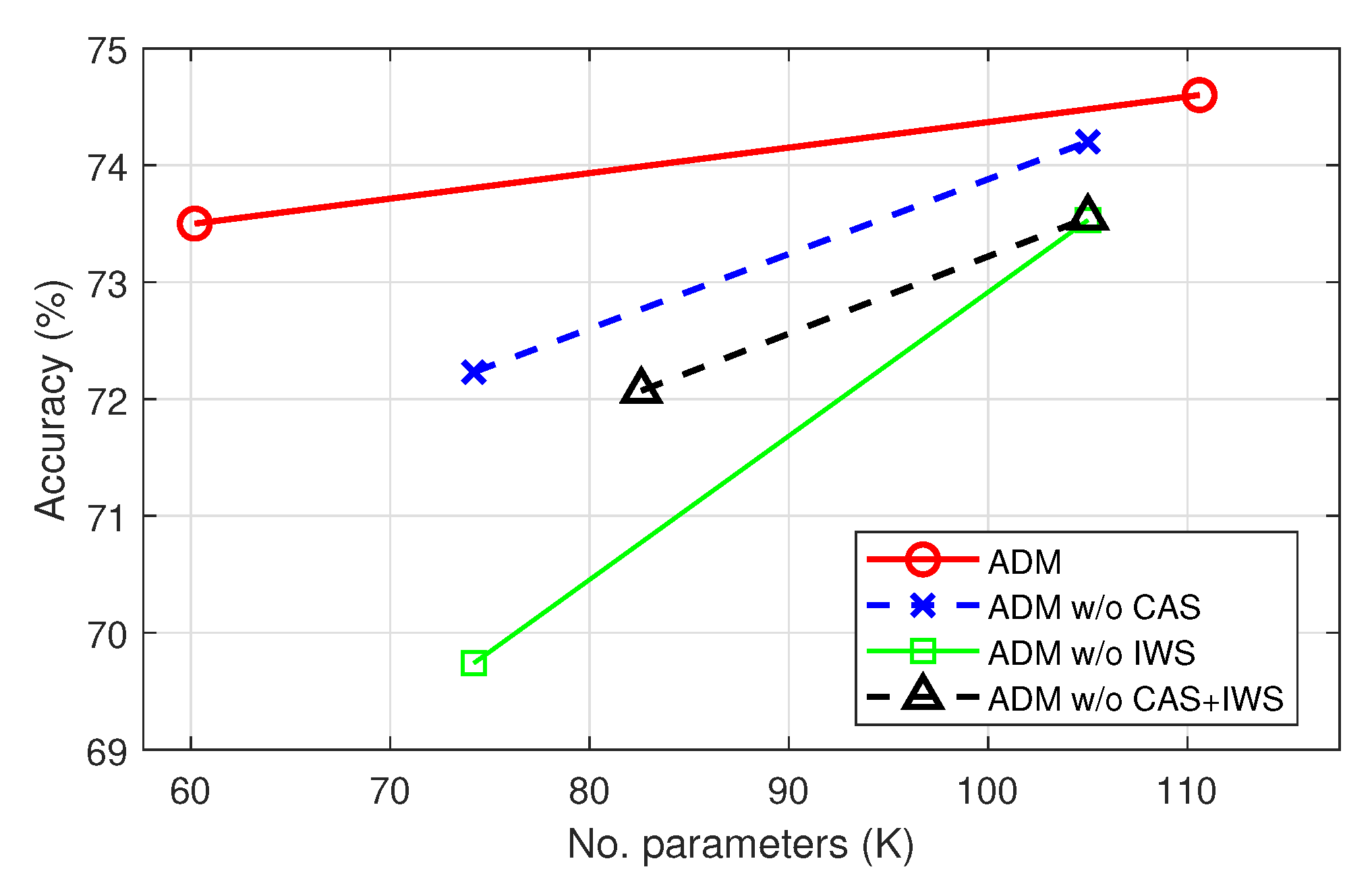
We also provide an ablation study of the proposed method on Mini-ImageNet in Scenario 4. Since ADM performs cost-adaptive search (CAS) and instance-wise search (IWS), we demonstrated the benefit of the proposed method compared with that without CAS, IWS, or both. Note that the problem of ADM without CAS (i.e., in Equation (6)) reduced to that of dynamic model search methods for multi-task learning [17,31]. Figure 8 shows the ablation study results. Overall, the proposed method (ADM) performed better than other approaches that do not perform CAS, IWS, or both. In particular, ADM without instance-wise search (green) gave a clear performance drop compared with ADM (red) and ADM without cost-adaptive search (blue). This shows the importance of instance-wise search, which can avoid negative interference among instances. Even though ADM without cost-adaptive search performed better than that without instance-wise search, it required individual training of multiple models corresponding to the number of computational costs. We can also observe that searching for a model of a single cost was more favorable when instance-wise search was not allowed. From the figure, we can see that the proposed method, which was able to perform cost-adaptive search in an instance-wise manner, gave excellent performance while producing a set of widely distributed solutions in a single trained architecture, making it highly efficient and competitive.
4.4.3. Average Model Structures of Different Computational Costs
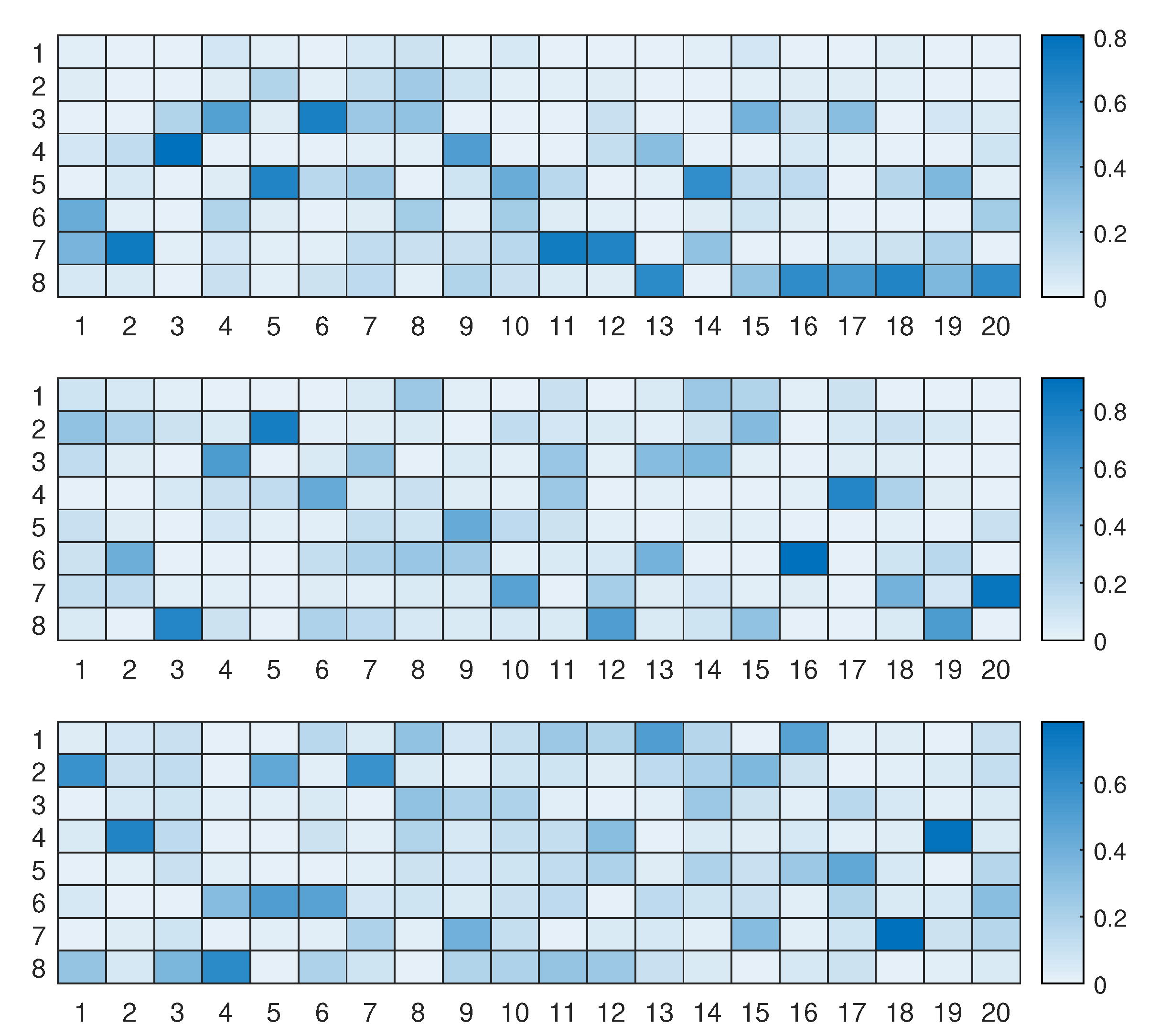
Lastly, we provide the average generated model structures under three different computational costs () for all test instances of a task (CIFAR-100) in Scenario 2, which are shown in Figure 9. For a higher computational cost, a larger number of building blocks was selected on average, whereas the search network selected a smaller number of building blocks for a lower computational budget, even though it chose nothing (denoted by 1 on the y axis) more frequently. We can also observe that the chosen model structures were quite dynamic for the same task (i.e., the selected building blocks were expressed in a wide range of the results). The average numbers of the selected building blocks (the total number of building blocks g was 3) in a ResBlock-M (and the average parameter densities) for the budgets were 2.2 (73%), 1.7 (57%), and 1.4 (45%) from top to bottom, respectively. This verifies the dynamic model search of the proposed method.
5. Conclusions
We presented ADM, a novel MTL approach for searching on-the-fly and cost-adaptive prediction models for each instance of a task. The proposed method can produce a set of widely distributed on-the-fly solutions, trading off between task performance and computation cost, and one can adaptively choose a suitable model for a given task with its required budget. To achieve the goal, we introduced a new modularized residual block, called ResBlock-M, that serves a rich search space and enables order-invariant searching for discovering a high-performance model. The effectiveness of the proposed method was validated for several MTL problems. Note that since the proposed method implicitly captures the relationship between tasks, it may be ineffective when learning a range of tasks. We will investigate possible directions to incorporate an explicit measure and consider the relevance between tasks in future work.
Funding
This research was supported in part by BK21 FOUR (Fostering Outstanding Universities for Research) Program funded by Ministry of Education of Korea (No.I22SS7609062) and in part by the Chung-Ang University Research Grants in 2021.
Institutional Review Board Statement
Not applicable.
Informed Consent Statement
Not applicable.
Data Availability Statement
Not applicable.
Conflicts of Interest
The author declares no conflict of interest.
References
- LeCun, Y.; Bengio, Y.; Hinton, G. Deep learning. Nature 2015, 521, 436–444. [Google Scholar] [CrossRef] [PubMed]
- Long, J.; Shelhamer, E.; Darrell, T. Fully convolutional networks for semantic segmentation. In Proceedings of the 2015 IEEE Conference on Computer Vision and Pattern Recognition (CVPR), Boston, MA, USA, 7–12 June 2015. [Google Scholar]
- Girshick, R. Fast R-CNN. In Proceedings of the 2015 IEEE International Conference on Computer Vision (ICCV), Santiago, Chile, 7–13 December 2015. [Google Scholar]
- He, K.; Zhang, X.; Ren, S.; Sun, J. Deep residual learning for image recognition. In Proceedings of the 2016 IEEE Conference on Computer Vision and Pattern Recognition (CVPR), Las Vegas, NV, USA, 27–30 June 2016. [Google Scholar]
- Bertinetto, L.; Valmadre, J.; Henriques, J.F.; Vedaldi, A.; Torr, P.H. Fully-convolutional siamese networks for object tracking. In Proceedings of the ECCV, Amsterdam, The Netherlands, 11–14 October 2016. [Google Scholar]
- Huang, G.; Liu, Z.; Weinberger, K.Q.; van der Maaten, L. Densely connected convolutional networks. In Proceedings of the 2017 IEEE Conference on Computer Vision and Pattern Recognition (CVPR), Honolulu, HI, USA, 21–26 July 2017. [Google Scholar]
- Simonyan, K.; Zisserman, A. Very deep convolutional networks for large-scale image recognition. In Proceedings of the 3rd International Conference on Learning Representations (ICLR 2015), San Diego, CA, USA, 7–9 May 2015. [Google Scholar]
- Kim, E.; Ahn, C.; Oh, S. NestedNet: Learning Nested Sparse Structures in Deep Neural Networks. In Proceedings of the 2018 IEEE/CVF Conference on Computer Vision and Pattern Recognition (CVPR), Salt Lake City, UT, USA, 18–23 June 2018. [Google Scholar]
- Caruana, R. Multitask learning. Mach. Learn. 1997, 28, 41–75. [Google Scholar] [CrossRef]
- Ruder, S. An overview of multi-task learning in deep neural networks. arXiv 2017, arXiv:1706.05098. [Google Scholar]
- Misra, I.; Shrivastava, A.; Gupta, A.; Hebert, M. Cross-stitch networks for multi-task learning. In Proceedings of the 2016 IEEE Conference on Computer Vision and Pattern Recognition (CVPR), Las Vegas, NV, USA, 27–30 June 2016. [Google Scholar]
- Kendall, A.; Gal, Y.; Cipolla, R. Multi-task learning using uncertainty to weigh losses for scene geometry and semantics. In Proceedings of the 2018 IEEE/CVF Conference on Computer Vision and Pattern Recognition (CVPR), Salt Lake City, UT, USA, 18–23 June 2018. [Google Scholar]
- Mallya, A.; Lazebnik, S. PackNet: Adding multiple tasks to a single network by iterative pruning. In Proceedings of the 2018 IEEE/CVF Conference on Computer Vision and Pattern Recognition (CVPR), Salt Lake City, UT, USA, 18–23 June 2018. [Google Scholar]
- Sun, X.; Panda, R.; Feris, R.; Saenko, K. Adashare: Learning what to share for efficient deep multi-task learning. Adv. Neural Inf. Process. Syst. 2020, 33, 8728–8740. [Google Scholar]
- Hazimeh, H.; Zhao, Z.; Chowdhery, A.; Sathiamoorthy, M.; Chen, Y.; Mazumder, R.; Hong, L.; Chi, E. Dselect-k: Differentiable selection in the mixture of experts with applications to multi-task learning. Adv. Neural Inf. Process. Syst. 2021, 34, 29335–29347. [Google Scholar]
- Raychaudhuri, D.S.; Suh, Y.; Schulter, S.; Yu, X.; Faraki, M.; Roy-Chowdhury, A.K.; Chandraker, M. Controllable Dynamic Multi-Task Architectures. In Proceedings of the IEEE/CVF Conference on Computer Vision and Pattern Recognition, New Orleans, LA, USA, 18–24 June 2022; pp. 10955–10964. [Google Scholar]
- Rosenbaum, C.; Klinger, T.; Riemer, M. Routing networks: Adaptive selection of non-linear functions for multi-task learning. In Proceedings of the 5th International Conference on Learning Representations (ICLR 2017), Toulon, France, 24–26 April 2017. [Google Scholar]
- Zhao, X.; Li, H.; Shen, X.; Liang, X.; Wu, Y. A Modulation Module for Multi-task Learning with Applications in Image Retrieval. In Proceedings of the ECCV, 15th European Conference, Munich, Germany, 8–14 September 2018. [Google Scholar]
- Donahue, J.; Jia, Y.; Vinyals, O.; Hoffman, J.; Zhang, N.; Tzeng, E.; Darrell, T. Decaf: A deep convolutional activation feature for generic visual recognition. In Proceedings of the ICML, 31st International Conference on International Conference on Machine Learning, Beijing, China, 21–26 June 2014. [Google Scholar]
- Yang, Y.; Hospedales, T.M. Trace norm regularised deep multi-task learning. arXiv 2016, arXiv:1606.04038. [Google Scholar]
- Jou, B.; Chang, S.F. Deep cross residual learning for multitask visual recognition. In Proceedings of the 24th ACM International Conference on Multimedia, ACM, Amsterdam, The Netherlands, 15–19 October 2016. [Google Scholar]
- Zamir, A.R.; Wu, T.L.; Sun, L.; Shen, W.B.; Shi, B.E.; Malik, J.; Savarese, S. Feedback networks. In Proceedings of the 2017 IEEE Conference on Computer Vision and Pattern Recognition (CVPR), Honolulu, HI, USA, 21–26 July 2017. [Google Scholar]
- Mallya, A.; Davis, D.; Lazebnik, S. Piggyback: Adapting a Single Network to Multiple Tasks by Learning to Mask Weights. In Proceedings of the ECCV, 15th European Conference, Munich, Germany, 8–14 September 2018. [Google Scholar]
- Kokkinos, I. Ubernet: Training a universal convolutional neural network for low-, mid-, and high-level vision using diverse datasets and limited memory. In Proceedings of the 2017 IEEE Conference on Computer Vision and Pattern Recognition (CVPR), Honolulu, HI, USA, 21–26 July 2017. [Google Scholar]
- Kim, E.; Ahn, C.; Torr, P.H.; Oh, S. Deep Virtual Networks for Memory Efficient Inference of Multiple Tasks. In Proceedings of the 2019 IEEE/CVF Conference on Computer Vision and Pattern Recognition (CVPR), Long Beach, CA, USA, 15–20 June 2019. [Google Scholar]
- Zoph, B.; Le, Q.V. Neural architecture search with reinforcement learning. In Proceedings of the 5th International Conference on Learning Representations (ICLR 2017), Toulon, France, 24–26 April 2017. [Google Scholar]
- Lin, J.; Rao, Y.; Lu, J.; Zhou, J. Runtime neural pruning. In Proceedings of the Advances in Neural Information Processing Systems, Long Beach, CA, USA, 4–9 December 2017; pp. 2181–2191. [Google Scholar]
- Wu, Z.; Nagarajan, T.; Kumar, A.; Rennie, S.; Davis, L.S.; Grauman, K.; Feris, R. Blockdrop: Dynamic inference paths in residual networks. In Proceedings of the 2018 IEEE/CVF Conference on Computer Vision and Pattern Recognition (CVPR), Salt Lake City, UT, USA, 18–23 June 2018. [Google Scholar]
- Liu, H.; Simonyan, K.; Yang, Y. Darts: Differentiable architecture search. In Proceedings of the 6th International Conference on Learning Representations (ICLR 2018), Vancouver, BC, Canada, 30 April–3 May 2018. [Google Scholar]
- Wang, X.; Yu, F.; Dou, Z.Y.; Darrell, T.; Gonzalez, J.E. Skipnet: Learning dynamic routing in convolutional networks. In Proceedings of the ECCV, 15th European Conference, Munich, Germany, 8–14 September 2018. [Google Scholar]
- Ahn, C.; Kim, E.; Oh, S. Deep Elastic Networks with Model Selection for Multi-Task Learning. In Proceedings of the 2019 IEEE/CVF International Conference on Computer Vision (ICCV), Seoul, Republic of Korea, 27 October–2 November 2019. [Google Scholar]
- Pham, H.; Guan, M.Y.; Zoph, B.; Le, Q.V.; Dean, J. Efficient neural architecture search via parameter sharing. In Proceedings of the 35th International Conference on Machine Learning (ICML 2018), Stockholm, Sweden, 10–15 July 2018. [Google Scholar]
- Howard, A.G.; Zhu, M.; Chen, B.; Kalenichenko, D.; Wang, W.; Weyand, T.; Andreetto, M.; Adam, H. MobileNets: Efficient convolutional neural networks for mobile vision applications. arXiv 2017, arXiv:1704.04861. [Google Scholar]
- Strezoski, G.; Noord, N.V.; Worring, M. Many task learning with task routing. In Proceedings of the 2019 IEEE/CVF International Conference on Computer Vision (ICCV), Seoul, Republic of Korea, 27 October–2 November 2019. [Google Scholar]
- Bragman, F.J.; Tanno, R.; Ourselin, S.; Alexander, D.C.; Cardoso, J. Stochastic filter groups for multi-task cnns: Learning specialist and generalist convolution kernels. In Proceedings of the IEEE International Conference on Computer Vision, Seoul, Republic of Korea, 27 October–2 November 2019; pp. 1385–1394. [Google Scholar]
- Zagoruyko, S.; Komodakis, N. Wide residual networks. In Proceedings of the British Machine Vision Conference (BMVC 2016), New York, NY, USA, 19–22 September 2016. [Google Scholar]
- Larsson, G.; Maire, M.; Shakhnarovich, G. FractalNet: Ultra-deep neural networks without residuals. In Proceedings of the 5th International Conference on Learning Representations (ICLR 2017), Toulon, France, 24–26 April 2017. [Google Scholar]
- Sutton, R.S.; McAllester, D.A.; Singh, S.P.; Mansour, Y. Policy gradient methods for reinforcement learning with function approximation. In Proceedings of the 13th International Conference on Neural Information Processing Systems, Cambridge, MA, USA, 1 January 2000. [Google Scholar]
- Metropolis, N.; Ulam, S. The monte carlo method. J. Am. Stat. Assoc. 1949, 44, 335–341. [Google Scholar] [CrossRef] [PubMed]
- Sutton, R.S.; Barto, A.G. Introduction to Reinforcement Learning; MIT Press Cambridge: Cambridge, UK, 1998; Volume 2. [Google Scholar]
- Krizhevsky, A.; Hinton, G. Learning Multiple Layers of Features from Tiny Images; Technical Report; University of Toronto: Toronto, ON, Canada, 2009. [Google Scholar]
- Coates, A.; Lee, H.; Ng, A.Y. An Analysis of Single Layer Networks in Unsupervised Feature Learning. In Proceedings of the AISTATS, 14th International Conference on Artificial Intelligence and Statistics, Ft. Lauderdale, FL, USA, 11–13 April 2011. [Google Scholar]
- Vinyals, O.; Blundell, C.; Lillicrap, T.; Wierstra, D. Matching networks for one shot learning. In Proceedings of the NIPS, Workshop on Interpretable Machine Learning for Complex Systems, Barcelona, Spain, 9 December 2016; pp. 3630–3638. [Google Scholar]
- Huang, G.; Sun, Y.; Liu, Z.; Sedra, D.; Weinberger, K.Q. Deep networks with stochastic depth. In Proceedings of the ECCV, 14th European Conference, Amsterdam, The Netherlands, 11–14 October 2016. 2016. [Google Scholar]
- Glorot, X.; Bengio, Y. Understanding the difficulty of training deep feedforward neural networks. In Proceedings of the 13th International Conference on Artificial Intelligence and Statistics (AISTATS 2010), Sardinia, Italy, 13–15 May 2010. [Google Scholar]
- Nesterov, Y. A method for unconstrained convex minimization problem with the rate of convergence O (1/k 2). Dokl. AN USSR 1983, 269, 543–547. [Google Scholar]
- Kingma, D.P.; Ba, J. Adam: A method for stochastic optimization. In Proceedings of the 2nd International Conference on Learning Representations, Banff, AB, Canada, 14–16 April 2014. [Google Scholar]
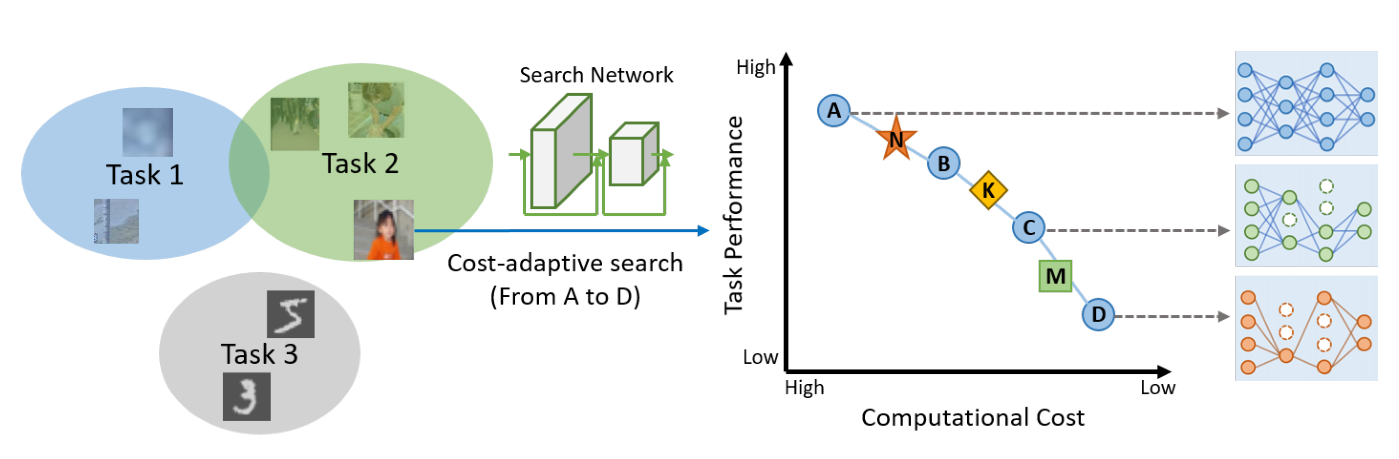
Figure 1.
A graphical illustration for a cost-adaptive search of the proposed approach on three tasks (classification datasets). For each instance of a task, ours method discovers a set of different models (represented by blue circles from A to D shown to the right of the figure) trading off between task performance and computational cost in the presented search network, whereas existing model search approaches can find only a single model (represented by either N, K, or M).

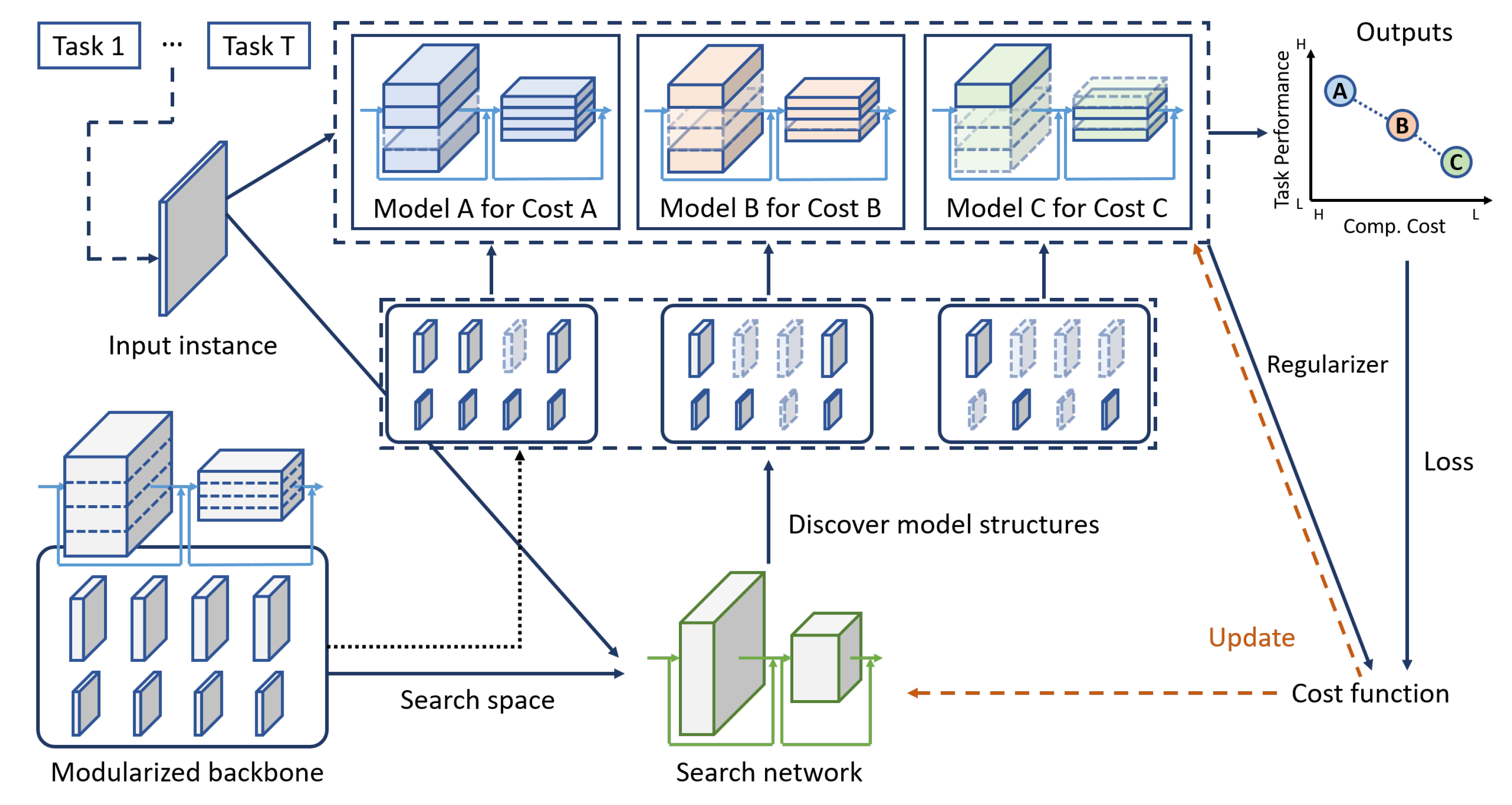
Figure 2.
Overall framework of the proposed method which consists of two major components: backbone and search networks. The proposed method updates the parameters (orange dotted lines) for the chosen models in the backbone and the search network by considering both task performance (loss) and computational cost (regularizer). The chosen models have trade-offs between task performance and computational cost shown in the top right.

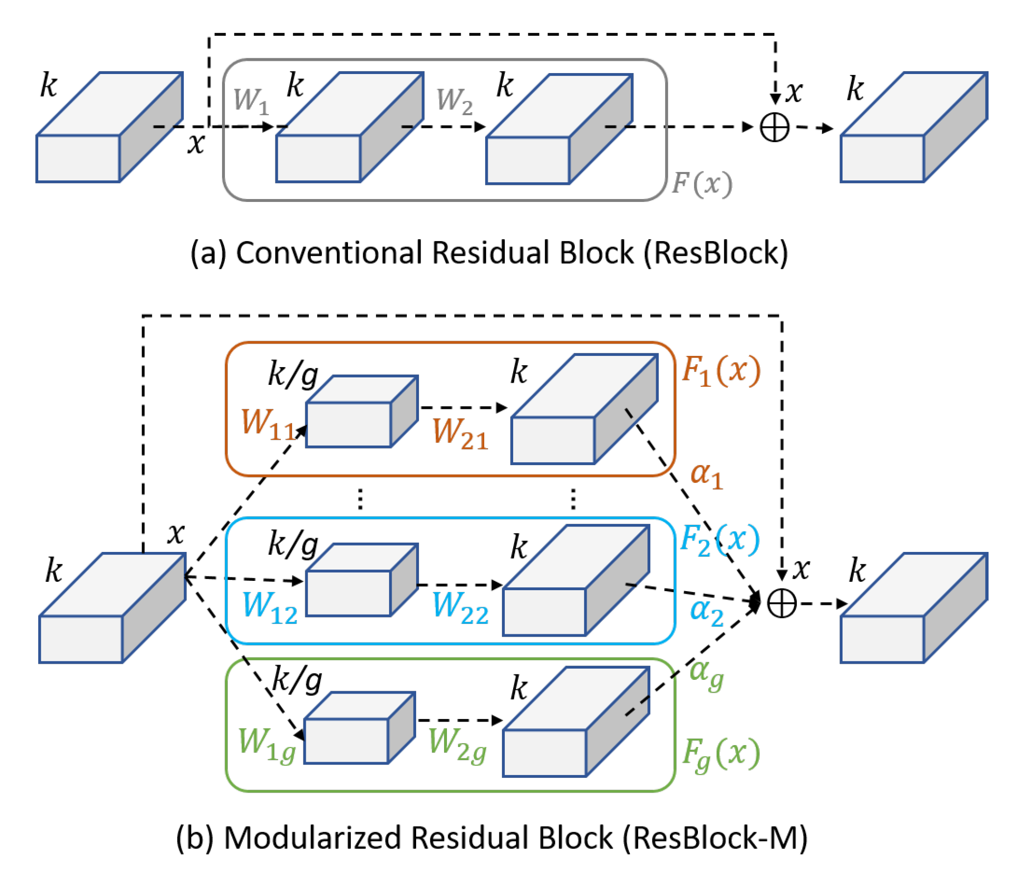
Figure 3.
(a) The conventional residual block (ResBlock) contains a single building block with its function , and the output is . (b) Our modularized residual block (ResBlock-M) contains g disjointed building blocks (represented by different colors) with their corresponding functions . The output is , where determines the usage of (best viewed in color).

Figure 4.
Classification results of the multi-task problem using the CIFAR-10 and CIFAR-100 datasets (two tasks). All the methods are based on the WRN-32-4 architecture, consuming 7.4 million parameters.
Figure 4.
Classification results of the multi-task problem using the CIFAR-10 and CIFAR-100 datasets (two tasks). All the methods are based on the WRN-32-4 architecture, consuming 7.4 million parameters.

Figure 5.
Classification results of the multi-task learning problem using three datasets (three tasks): CIFAR-100, Tiny-ImageNet, and STL-10. All the methods are based on ResNet-42 (29.8 million parameters).
Figure 5.
Classification results of the multi-task learning problem using three datasets (three tasks): CIFAR-100, Tiny-ImageNet, and STL-10. All the methods are based on ResNet-42 (29.8 million parameters).

Figure 6.
The selected model structures for three images of different tasks. The backbone architecture is ResNet-42, which contains 20 ResBlock-M, indicated on the x axis. The number of building blocks is three, thus we have choices for the building blocks in each ResBlock-M (e.g., 1 indicates nothing is chosen, and 8 indicates all the building blocks are selected on the y axis). The difficulty of the images decreases from top to bottom.

Figure 7.
Qualitative results of the proposed method for Scenario 2 (three tasks). Given a query (standalone) image from each task, we drew similar images whose selected model structures were almost similar to that of the query image. Similar images from the top to bottom rows were from Tasks 1–3, respectively. Best viewed in color (×2).

Figure 8.
Ablation study on Mini-ImageNet. The results of the dotted lines were collected from independently trained models. CAS = cost-adaptive search, and IWS = instance-wise search.
Figure 8.
Ablation study on Mini-ImageNet. The results of the dotted lines were collected from independently trained models. CAS = cost-adaptive search, and IWS = instance-wise search.

Figure 9.
Average of the selected model structures for the CIFAR-100 test datasets in Scenario 2 under three different computational budgets (), which decrease from top to bottom. The backbone architecture was ResNet-42, which contains 20 ResBlock-Ms, indicated on the x axis. The number of building blocks was three, and thus we had eight choices for the building blocks in each ResBlock-M.


Table 1.
Algorithmic comparison of the dynamic search methods with respect to different functionalities: multi-task learning (MTL), cost-adaptive search (CAS), and instance-wise search (IwS). Here, g and r are the numbers of groups (or channels) and residual blocks, respectively, and l and e are the numbers of layers and experts in each layer, respectively.
| Method | MTL | CAS | IwS | Search Space |
|---|---|---|---|---|
| RNP [27] | ✗ | ✓ | ✓ | |
| RoutingNet [17] | ✓ | ✗ | ✗ | |
| SkipNet [30] | ✗ | ✗ | ✓ | |
| BlockDrop [28] | ✗ | ✗ | ✓ | |
| VirtualNet [25] | ✓ | ✗ | ✗ | g |
| DEN [31] | ✓ | ✗ | ✓ | |
| MT-SGF [35] | ✓ | ✗ | ✗ | |
| TRL [34] | ✓ | ✗ | ✗ | |
| Ours | ✓ | ✓ | ✓ |
Table 2.
Summary of four experimental scenarios with the corresponding architectures.
| Scenario | No. Tasks | Datasets | Architecture |
|---|---|---|---|
| 1 | 2 | CIFAR-10, CIFAR-100 | WRN-32-4 |
| 2 | 3 | CIFAR-100, Tiny-ImageNet, STL-10 | ResNet-42 |
| 3 | 20 | CIFAR-MTL | SimpleConvNet |
| 4 | 10 | Mini-ImageNet | SimpleConvNet |
Table 3.
Average classification results with the numbers of parameters of the compared methods for CIFAR-MTL (20 tasks). The accuracies of the other methods were borrowed from [17].
Table 3.
Average classification results with the numbers of parameters of the compared methods for CIFAR-MTL (20 tasks). The accuracies of the other methods were borrowed from [17].
| Accuracy | Number of Parameters | |
|---|---|---|
| Baseline | 42.0% | 74,000 |
| Cross-stitch network [11] | 54.0% | 74,000↑ |
| Routing network [17] | 61.0% | 74,000 |
| ADM (ours) | 65.5% | 38,000 |
| 67.6% | 56,000 |
Table 4.
Average classification results with the numbers of parameters of the compared methods for Mini-ImageNet (10 tasks). The accuracies of the other methods were borrowed from [17].
Table 4.
Average classification results with the numbers of parameters of the compared methods for Mini-ImageNet (10 tasks). The accuracies of the other methods were borrowed from [17].
| Accuracy | Number of Parameters | |
|---|---|---|
| Baseline | 51.0% | 140,000 |
| Cross-stitch network [11] | 56.0% | 140,000↑ |
| Routing network [17] | 59.0% | 140,000 |
| ADM (ours) | 73.5% | 60,000 |
| 74.6% | 110,000 |
Publisher’s Note: MDPI stays neutral with regard to jurisdictional claims in published maps and institutional affiliations. |
© 2022 by the author. Licensee MDPI, Basel, Switzerland. This article is an open access article distributed under the terms and conditions of the Creative Commons Attribution (CC BY) license (https://creativecommons.org/licenses/by/4.0/).
Share and Cite
MDPI and ACS Style
Kim, E. Adaptive Dynamic Search for Multi-Task Learning. Appl. Sci. 2022, 12, 11836. https://doi.org/10.3390/app122211836
AMA Style
Kim E. Adaptive Dynamic Search for Multi-Task Learning. Applied Sciences. 2022; 12(22):11836. https://doi.org/10.3390/app122211836
Chicago/Turabian StyleKim, Eunwoo. 2022. "Adaptive Dynamic Search for Multi-Task Learning" Applied Sciences 12, no. 22: 11836. https://doi.org/10.3390/app122211836
Note that from the first issue of 2016, this journal uses article numbers instead of page numbers. See further details here.