An Analytical Solution to Steady-State Temperature Field in the FSPR Method Considering Different Soil Freezing Points

Abstract

Taking the freeze-sealing pipe roof method (FSPR) adopted in the Gongbei Tunnel project as the background, this study develops a simplified calculation model by considering different soil freezing points, tube layout, and site conditions. The analytical solution of the linear single row tubes is then used to formulate the analytical solution of the freezing temperature field of two kinds of linear single row tubes, with equal spacing in the image plane. This is achieved through conformal mapping and the variable separation method. Finally, the analytical solution to the steady-state temperature field of FSPR in the object plane is obtained. The numerical solutions of common freezing parameters in freezing engineering are analyzed to evaluate the accuracy of the analytical solution, and the influence of parameter differences on the freezing temperature field are also discussed, to provide a theoretical reference for popularization and application of similar construction methods.

1. Introduction

The theoretical analysis of artificial freezing temperature fields has been extensively investigated in the ground freezing engineering field, particularly in heat conduction problems, including “phase transition”, “hydrothermal coupling”, “temporal and spatial effect” and other factors [1,2]. The currently applied research methods include analytical, experimental and numerical methods [3,4,5,6,7]. These analytical methods use mathematical and physical equations to establish accurate functional relationships for research problems. The relationships between variables in the function are clear and can be directly solved, and they can be applied by engineers and technicians during the design stage and to evaluate the effect of on-site freezing construction. Therefore, they can be utilized to study artificial freezing temperature fields [8,9,10]. However, considering the differences in the number and arrangement of freezing tubes, freezing front movement, water migration and other factors, the analytical method still has some limitations when applied in mathematical solutions, and can only analyze the temperature field of single tube freezing. In academic and engineering fields, many cases [11] have confirmed that the artificial freezing temperature field develops very slowly, at the final stage of the freezing process. Since the freezing tube will have reached the equilibrium state of cooling and heat absorption, the size of the frozen wall almost does not change, and would be very close to the steady-state heat transfer temperature field [12]. Therefore, the steady-state heat transfer model can be used for approximate calculation.

Extensive research and derivation have been performed on the analytical solutions of freezing steady-state temperature field. Currently, the commonly used analytical solutions include the single-tube freezing steady-state temperature field [13], the two-to-five-tube equidistant linear arrangement steady-state temperature field [14,15,16] presented by Bakholdin, the symmetric and asymmetric steady-state temperature fields of linear single-row tubes [17], linear double-row tubes and three-row tubes [18,19,20], and the annular single- circle-tube and double- circle-tube temperature field [21,22]. The aforementioned results are based on the classic Trupak single-tube freezing steady-state temperature field analytical solution formula, obtained through potential function superposition, separation variable method, conformal mapping and other processing methods, combined with practical engineering situations to simplify the corresponding model, and improve its application value in engineering. However, with the continuous and rapid development of urban construction in China, higher requirements have been proposed regarding the formation and functioning of underground engineering structures. For many engineering fields that involve difficult construction, it is challenging to establish strong support methods to handle complex geological conditions. Most analytical solutions also need to be constantly revised or optimized to meet higher requirements such as various geological conditions, accurate and fast calculation of temperature and frozen soil curtain thickness [23,24,25]. Therefore, continuous in-depth studies should be performed to establish a theoretical basis that is in line with engineering practices.

To overcome the challenges associated with constructing shallow buried and concealed excavation tunnels with large sections in the water-rich soft soil of coastal cities, Chinese experts and scholars have put forward a new tunnel construction method; the freeze-sealing pipe roof method (FSPR) that integrates the pipe roof method (PRM) and the artificial ground freezing method (AGF) [26,27]. In Figure 1, a plurality of closely arranged large-diameter steel pipes are jacked into the strata at both ends of the tunnel section to form a pipe roof. Subsequently, the surrounding water-containing soft soil layer is artificially frozen by installing a freezing tube in the inner wall of the jacking pipe. A closed freezing curtain is created within the scope of the tunnel excavation section, which finally constitutes a large-scale composite support structure of “frozen soil curtain and jacking pipe” [28].

In Figure 1, the underground excavation section of the Gongbei Tunnel, the key project of the Zhuhai link of the Hong Kong-Zhuhai-Macao Bridge in China, achieved successful application of FSPR for the first time in the world, with good engineering results. In the construction scheme of this project, artificial ground freezing technology was used to freeze the ground to form a frozen soil curtain, thereby sealing the water between the pipes and improving the bearing capacity of the pipe roof. The freezing construction period takes 180 days, and considering the damage caused by excessive frost heaving, the thickness of the frozen soil curtain is designed in advance, and the cooling capacity is strictly controlled [29]. According to the field measured data, after 90 days of freezing, the thickness of the frozen soil curtain remains unchanged, because the cooling supply and heat absorption of the freezing tube reach a state of balance, so the temperature field after that can be regarded as a quasi-steady state. Model analysis and calculation of the freezing temperature field is the basis of theoretical research on FSPR, which can provide strong support for similar methods in freezing construction parameter designs, process monitoring, and target prediction [30]. During the whole freezing construction process, it is necessary to grasp the frozen soil curtain thickness and temperature distribution law based on the calculation and analysis of the temperature field, and to evaluate the reliability of water sealing between pipes [31].

In this article, inspired by the existing analytical results and to better adapt to the complex ground freezing conditions in the practical project, we have established a simplified model by considering different soil freezing points and tube placement forms of FSPR. Through the conformal mapping function and separation of variables solution, the analytical solution of the freezing temperature field of two kinds of freezing tubes with equal spacing in a straight line in the image plane is derived, after which the analytical solution of steady-state temperature field in the object plane is obtained. The accuracy of the analytical solution is verified by comparing the numerical solution of this project in the range of soil freezing point 0~−1.5 °C, and the influence of the parameter differences on the freezing temperature field is also discussed to provide a theoretical reference for popularization and applications of similar construction methods.

2. Establishment of the Calculation Model for FSPR Steady State Temperature Field

2.1. Model Simplifications and Assumptions

In Figure 2, 18 concrete pipes and 18 hollow pipes were alternately arranged to form a super-large section pipe roof during the freezing construction of the pipe curtain of Gongbei Tunnel. The arrangement axis of the 18 hollow top pipes is a 5-segment circular arc with left and right symmetry, while the arc lengths and radii are Arc₁ = 5.45 m and R₁ = 9.86, Arc₂ = 4.87 m and R₂ = 6.96 m, Arc₃ = 11.75 m and R₃ = 20.96 m, Arc₄ = 3.86 m and R₄= 3.86 m, Arc₅ = 6.17 m and R₅ = 18.86 m, respectively. The axes of the 18 concrete pipes are offset by 30 cm inward, thus, there is a slight dislocation of the circular freezing tubes in concrete pipes, and of the profiled freezing tubes in hollow pipes. The soil between the pipes is frozen through the cryogenic refrigerant circulation method in these two types of freezing tubes. The limiting tube is arranged on the outside of the axis of the concrete pipe; excess cold can be removed by circulating hot brine in the tube, while the thickness of the outside of the frozen soil curtain can be controlled to reduce frost heave of the stratum. The structural form and function of the FSPR method are extremely complex, therefore, appropriate assumptions and model simplification are required to ensure the feasibility of the analytical solution of the steady-state temperature field, including:

(1)

The entire length of the underground excavation section of the Gongbei Tunnel is 255 m long and is curved. The actual tube curtain freezing is a three-dimensional heat conduction problem. The temperature deviation of longitudinal freezing is ignored, and it can be simplified to a two-dimensional plane problem.

(2)

Ignoring the irregular shape of the pipe curtain section and the slight offset between the hollow and concrete pipe axes, all 36 pipes are considered to be arranged on the same circumferential line, that is, the pipe curtain section is simplified to a circle.

(3)

In the actual project, due to the arrangement of the pipes, the outline of the frozen soil curtain is irregularly wavy. Considering the steady-state temperature field, the end of the freezing process is studied. For mathematical derivation convenience, it is assumed that the contour line of the frozen soil curtain is approximately a circle, and its rationality can be evaluated by verifying the analytical solution.

(4)

The profiled freezing tube in the hollow pipe contains a non-circular section, and its size is smaller compared with that of the jacking pipe. It is estimated to have the same section and size as the circular freezing tube in the concrete pipe. Flow and temperature differences of the low-temperature refrigerant in the two types of freezing pipes in the freezing process are ignored, and only the two types of freezing tubes with the same tube wall temperature are considered during derivation of the analytical solution. The effects of hollow and concrete pipes on the freezing temperature field are also ignored, and only the effects of freezing tubes are considered.

Based on the above assumptions, the model in Figure 2 is simplified, and freezing tubes as well as frozen soil curtains are selected as the main research objects [32]. Two types of freezing tubes, A and B, with radii R₀ are obtained, which are periodically arranged on the circumference line (R₂), and the spacing is set as the dislocation angle β. The inner and outer boundaries (R₁ and R₃) of the frozen soil curtain are circular (Figure 3):

In Figure 3, the appropriate cartesian coordinate system is selected so that the center of a type A freezing tube is just on the positive semi-axis of the x-axis. Next, the corresponding mathematical expression of the two-dimensional steady-state temperature field is calculated using Equation group (1):

$$\left\{\begin{array}{l}\frac{{\partial }^{2}T}{\partial r^2}+\frac{1}{r}\frac{\partial T}{\partial r}+\frac{{\partial }^{2}T}{\partial {\theta }^2}=0;\text{Two-dimensional} \text{steady-state} \mathrm{heat} \mathrm{conduction} \mathrm{equation}\\ T(R_2+R_0,k\frac{2\pi }{n})=T_f;\mathrm{Boundary} \mathrm{condition} \mathrm{for} \text{A-type} \mathrm{freezing} \mathrm{tubes}\\ T(R_2+R_0,k\frac{2\pi }{n}-\beta )=T_f;\mathrm{Boundary} \mathrm{condition} \mathrm{for} \text{B-type} \mathrm{freezing} \mathrm{tubes}\\ T(R_1,k\frac{2\pi }{n})=T_0;\mathrm{Inner} \mathrm{boundary} \mathrm{conditions} \mathrm{for} \mathrm{frozen} \mathrm{soil} \mathrm{curtain},T_0\ne 0\\ T(R_3,k\frac{2\pi }{n})=T_0;\mathrm{Outer} \mathrm{boundary} \mathrm{conditions} \mathrm{for} \mathrm{frozen} \mathrm{soil} \mathrm{curtain},T_0\ne 0\end{array}\right.$$

(1)

where:

$$\begin{array}{ccc}\hfill r,\theta & —& \mathrm{Polar} \mathrm{diameter} \mathrm{and} \mathrm{polar} \mathrm{angle}\hfill \\ \hfill T_0,T_f& —& \mathrm{Frozen} \mathrm{curtain} \mathrm{boundary} \mathrm{temperature} \mathrm{and} \mathrm{freezing} \mathrm{tube} \mathrm{wall} \mathrm{temperature}\hfill \\ \hfill n,R_0& —& \mathrm{Number} \mathrm{and} \mathrm{radius} \mathrm{of} \mathrm{type} \mathrm{A} \mathrm{and} \mathrm{B} \mathrm{freezing} \mathrm{tubes}\hfill \\ \hfill k& —& \mathrm{Values} \mathrm{from} 0 \mathrm{to} \mathrm{n}-1\hfill \\ \hfill R_1,R_3& —& \mathrm{Inner} \mathrm{and} \mathrm{outer} \mathrm{boundary} \mathrm{radii} \mathrm{of} \mathrm{frozen} \mathrm{curtain}\hfill \\ \hfill R_2& —& \mathrm{Freezing} \mathrm{tube} \mathrm{arrangement} \mathrm{circle} \mathrm{diameter}\hfill \\ \hfill \beta & —& \mathrm{Dislocation} \mathrm{angle} \mathrm{between} \mathrm{two} \mathrm{adjacent} \mathrm{freezing} \mathrm{tubes}\hfill \end{array}$$

2.2. Conformal Mapping and Calculation Model Transformation

Considering that it is difficult to directly solve Equation group 1, conformal mapping should be considered during the conversion of circular boundary conditions of the model into the corresponding linear boundary conditions, thus, the logarithmic transformation function is introduced [33,34]:

$$\left\{\begin{array}{l}\zeta =i\ln \left(\frac{Z}{R_2}\right)\\ Z=r{e}^{i\theta };\mathrm{Object} \mathrm{plane}\\ \zeta =x+iy;\mathrm{Image} \mathrm{plane}\end{array}\right.$$

(2)

where by Z represents the object plane (i.e., the original plane in Figure 3), r and θ represent a point in the object plane, ζ represent the image plane, x and y represent a point in the image plane, we can obtain:

$$x+iy=-\theta +i\ln \left(\frac{r}{R_2}\right)$$

(3)

From Equations (2) and (3), we can convert the computational model in Figure 3 into the non-equidistant single-row tube with asymmetric development of the frozen curtain in the image plane, as shown in Figure 4:

This model can be calculated using Equation groups (4) and (5):

$$\left\{\begin{array}{l}x=-\theta ,y=\ln \frac{r}{R_2}\\ {\xi }_1=\ln \frac{R_2}{R_1},{\xi }_2=\ln \frac{R_3}{R_2}\\ l=\frac{2\pi }{n},d=\beta ,r_0=\frac{R_0}{R_2}\end{array}\right.$$

(4)

$$\left\{\begin{array}{l}\frac{{\partial }^{2}T}{\partial x^2}+\frac{{\partial }^{2}T}{\partial y^2}=0\\ T(nl,r_0)=T_f;\mathrm{Boundary} \mathrm{condition} \mathrm{for} \text{A′-type} \mathrm{freezing} \mathrm{tubes}\\ T(d+nl,r_0)=T_f;\mathrm{Boundary} \mathrm{condition} \mathrm{for} \text{B′-type} \mathrm{freezing} \mathrm{tubes}\\ T(x,{\xi }_2)=T_0;\mathrm{Frozen}\mathrm{soil}\mathrm{boundary}\mathrm{II},T_0\ne 0\\ T(x,-{\xi }_1)=T_0;\mathrm{Frozen}\mathrm{soil}\mathrm{boundary}\mathrm{I},T_0\ne 0\end{array}\right.$$

(5)

where by, Equation group (4) denotes the conformal mapping function relationship between the models in Figure 3 and Figure 4. Equation group (5) denotes the expressions of the model in Figure 4.

If the two types of freezing tubes A′ and B′ are separated, two linear single-row tubes’ (equidistantly spaced) models of asymmetric frozen soil curtains can be obtained. Therefore, based on the separation variable solution method [35,36,37], the model in Figure 4 is regarded as a superposition of the two types of linear single-row tube equidistant arrangement models A′ and B′ (Figure 5):

Mathematical expressions of A′-type and B′-type linear single-row tube models are shown in Equation groups (6) and (7), respectively:

$$\left\{\begin{array}{l}\frac{{\partial }^2{T}_1}{\partial x^2}+\frac{{\partial }^2{T}_1}{\partial y^2}=0\\ T_1(nl,r_0)=T_f-a;\mathrm{Boundary} \mathrm{condition} \mathrm{for} \text{A′-type} \mathrm{freezing} \mathrm{tubes}\\ T_1(d+nl,r_0)=b;\mathrm{Boundary} \mathrm{condition} \mathrm{for} \text{B′-type} \mathrm{freezing} \mathrm{tubes}\\ T_1(nl,{\xi }_2)=T_0;\mathrm{Frozen}\mathrm{soil}\mathrm{boundary}\mathrm{II},T_0\ne 0\\ T_1(nl,-{\xi }_1)=T_0;\mathrm{Frozen}\mathrm{soil}\mathrm{boundary}\mathrm{I},T_0\ne 0\end{array}\right.$$

(6)

$$\left\{\begin{array}{l}\frac{{\partial }^2{T}_2}{\partial x^2}+\frac{{\partial }^2{T}_2}{\partial y^2}=0\\ T_2(nl,r_0)=a;\mathrm{Boundary} \mathrm{condition} \mathrm{for} \text{A′-type} \mathrm{freezing} \mathrm{tubes}\\ T_2(d+nl,r_0)=T_f-b;\mathrm{Boundary} \mathrm{condition} \mathrm{for} \text{B′-type} \mathrm{freezing} \mathrm{tubes}\\ T_2(nl,{\xi }_2)=T_0;\mathrm{Frozen}\mathrm{soil}\mathrm{boundary}\mathrm{II},T_0\ne 0\\ T_2(nl,-{\xi }_1)=T_0;\mathrm{Frozen}\mathrm{soil}\mathrm{boundary}\mathrm{I},T_0\ne 0\end{array}\right.$$

(7)

where the model temperature field T (Equation group (5)) is the superposition of temperature fields T₁ and T₂ of two different frozen soil boundary conditions, namely: T = T₁ + T₂. a and b are the coefficients to be solved.

2.3. Analytical Solution for Freezing Temperature Field Model in the Image Plane of Non-Equidistant Single-Row Tube with Asymmetric Development of Frozen Curtain

For the A′-type model in Figure 5a, according to Bakholdin’s single-row tube freezing model theory and characteristics of asymmetric frozen soil curtains, the general form of its steady-state analytical solution can be obtained as:

$$T=\frac{T_f-T_0}{\ln \frac{2\pi r_0}{l}-\frac{\pi }{l}\cdot \frac{2{\xi }_1{\xi }_2}{{\xi }_1+{\xi }_2}}\left\{\frac{1}{2}\ln \left[2(\cosh \frac{2\pi y}{l}-\cos \frac{2\pi x}{l})\right]-\frac{\pi }{l}\cdot \frac{2{\xi }_1{\xi }_2}{{\xi }_1+{\xi }_2}+\frac{\pi }{l}\cdot \frac{{\xi }_1-{\xi }_2}{{\xi }_1+{\xi }_2}y\right\}+T_0$$

(8)

Using Equation (8), the solution for Equation group (6) can be obtained as:

$$T_1=\frac{T_f-a-T_0}{\ln \frac{2\pi r_0}{l}-\frac{\pi }{l}\cdot \frac{2{\xi }_1{\xi }_2}{{\xi }_1+{\xi }_2}}\left\{\frac{1}{2}\ln \left[2(\cosh \frac{2\pi y}{l}-\cos \frac{2\pi x}{l})\right]-\frac{\pi }{l}\cdot \frac{2{\xi }_1{\xi }_2}{{\xi }_1+{\xi }_2}+\frac{\pi }{l}\cdot \frac{{\xi }_1-{\xi }_2}{{\xi }_1+{\xi }_2}y\right\}+T_0$$

(9)

Substituting the boundary condition for B′-type freezing tubes in Equation group (6) into Equation (9), we get:

$$b=\frac{T_f-a-T_0}{\ln \frac{2\pi r_0}{l}-\frac{\pi }{l}\cdot \frac{2{\xi }_1{\xi }_2}{{\xi }_1+{\xi }_2}}\left\{\frac{1}{2}\ln \left[2(\cosh \frac{2\pi r_0}{l}-\cos \frac{2\pi (d+nl)}{l})\right]-\frac{\pi }{l}\cdot \frac{2{\xi }_1{\xi }_2}{{\xi }_1+{\xi }_2}+\frac{\pi }{l}\cdot \frac{{\xi }_1-{\xi }_2}{{\xi }_1+{\xi }_2}{r}_0\right\}+T_0$$

(10)

In the same way, the B′-type model in Figure 5b is equivalent to the A′-type model where each freezing tube is shifted to the right by a distance d. From Equation (8), the solution for Equation group (7) can be obtained as:

$$T_2=\frac{T_f-b-T_0}{\ln \frac{2\pi r_0}{l}-\frac{\pi }{l}\cdot \frac{2{\xi }_1{\xi }_2}{{\xi }_1+{\xi }_2}}\left\{\frac{1}{2}\ln \left[2(\cosh \frac{2\pi y}{l}-\cos \frac{2\pi (x-d)}{l})\right]-\frac{\pi }{l}\cdot \frac{2{\xi }_1{\xi }_2}{{\xi }_1+{\xi }_2}+\frac{\pi }{l}\cdot \frac{{\xi }_1-{\xi }_2}{{\xi }_1+{\xi }_2}y\right\}+T_0$$

(11)

Substituting the boundary condition for A′-type freezing tubes in Equation group (7) into Equation (11), we get:

$$a=\frac{T_f-b-T_0}{\ln \frac{2\pi r_0}{l}-\frac{\pi }{l}\cdot \frac{2{\xi }_1{\xi }_2}{{\xi }_1+{\xi }_2}}\left\{\frac{1}{2}\ln \left[2(\cosh \frac{2\pi r_0}{l}-\cos \frac{2\pi (nl-d)}{l})\right]-\frac{\pi }{l}\cdot \frac{2{\xi }_1{\xi }_2}{{\xi }_1+{\xi }_2}+\frac{\pi }{l}\cdot \frac{{\xi }_1-{\xi }_2}{{\xi }_1+{\xi }_2}{r}_0\right\}+T_0$$

(12)

Since Equations (10) and (12) are relatively complex, they are simplified before the simultaneous solution:

$$\left\{\begin{array}{c}a=(T_f-b-T_0)\frac{{\eta }_{\zeta }}{{\phi }_{\zeta }}+T_0\\ b=(T_f-a-T_0)\frac{{\eta }_{\zeta }}{{\phi }_{\zeta }}+T_0\end{array}\right.$$

(13)

where:

$${\eta }_{\zeta }=\frac{1}{2}\ln \left[2(\cosh \frac{2\pi r_0}{l}-\cos \frac{2\pi d}{l})\right]-\frac{\pi }{l}\cdot \frac{2{\xi }_1{\xi }_2}{{\xi }_1+{\xi }_2}+\frac{\pi }{l}\cdot \frac{{\xi }_1-{\xi }_2}{{\xi }_1+{\xi }_2}{r}_0$$

$${\phi }_{\xi }=\ln \frac{2\pi r_0}{l}-\frac{\pi }{l}\cdot \frac{2{\xi }_1{\xi }_2}{{\xi }_1+{\xi }_2}$$

Equation group (13) is solved to get:

$$a=b=\frac{T_f\frac{{\eta }_{\zeta }}{{\phi }_{\zeta }}+T_0(1-\frac{{\eta }_{\zeta }}{{\phi }_{\zeta }})}{1+\frac{{\eta }_{\zeta }}{{\phi }_{\zeta }}}$$

(14)

Substitute Equation (14) into Equations (9) and (11) respectively, and according to T = T₁ + T₂, we get:

$$T=\frac{{\gamma }_{\zeta }}{{\phi }_{\zeta }+{\eta }_{\zeta }}\cdot (T_f-2T_0)+2T_0$$

(15)

where:

$${\gamma }_{\zeta }=\frac{1}{2}\ln \left[2(\cosh \frac{2\pi y}{l}-\cos \frac{2\pi x}{l})\right]+\frac{1}{2}\ln \left[2(\cosh \frac{2\pi y}{l}-\cos \frac{2\pi (x-d)}{l})\right]-\frac{2\pi }{l}\cdot \frac{2{\xi }_1{\xi }_2}{{\xi }_1+{\xi }_2}+\frac{2\pi }{l}\cdot \frac{{\xi }_1-{\xi }_2}{{\xi }_1+{\xi }_2}y$$

(16)

Equation (16) is the analytical solution for the freezing temperature field model in the image plane of a non-equidistant single-row tube with asymmetric development of the frozen curtain shown in Figure 4.

2.4. Analytical Solution for Freezing Temperature Field Model in Object Plane of FSPR

Substituting Equation group (4) into Equation (16), we get:

$$T=\frac{{\gamma }_Z}{{\phi }_Z+{\eta }_Z}\cdot (T_f-2T_0)+2T_0$$

(17)

where:

$${\gamma }_Z=\frac{1}{2}\ln \left[{\left(\frac{r}{R_2}\right)}^n+{\left(\frac{R_2}{r}\right)}^n-2\cos n\theta \right]+\frac{1}{2}\ln \left[{\left(\frac{r}{R_2}\right)}^n+{\left(\frac{R_2}{r}\right)}^n-2\cos n(\theta +\beta )\right]-\frac{2n\ln \frac{R_2}{R_1}\ln \frac{R_3}{R_2}}{\ln \frac{R_3}{R_1}}+\frac{n\ln \frac{R_2^2}{R_1{R}_3}}{\ln \frac{R_3}{R_1}}\cdot \ln \frac{r}{R_2}$$

$${\phi }_Z=\ln \frac{n{R}_0}{R_2}-\frac{n\ln \frac{R_2}{R_1}\ln \frac{R_3}{R_2}}{\ln \frac{R_3}{R_1}}$$

$${\eta }_Z=\frac{1}{2}\ln \left(e^{\frac{n{R}_0}{R_2}}+e^{-\frac{n{R}_0}{R_2}}-2\cos n\beta \right)-\frac{n\ln \frac{R_2}{R_1}\ln \frac{R_3}{R_2}}{\ln \frac{R_3}{R_1}}+\frac{n\ln \frac{R_2^2}{R_1{R}_3}}{2\ln \frac{R_3}{R_1}}\cdot \frac{R_0}{R_2}$$

Equation (17) is the analytical solution to steady-state temperature field of FSPR when considering different soil freezing points as shown in Figure 3.

3. Accuracy Verification of the Analytical Solution

3.1. Selection of Feature Parameters

For the calculation model of FSPR in Figure 3, since the freezing tubes are periodically arranged, take an A-type freezing tube and a B-type freezing tube adjacent to the x-axis as research objects. Taking the origin of coordinates as the center of the circle, select the fan-shaped area as shown in Figure 6 for calculation.

Select the x-axis direction (main section, θ = 0), between two pipes (Section 1, θ = −β/2), and the sector boundary (Section 2, θ = π/n − β/2) as the three characteristic sections for temperature calculation, ξ₁ and ξ₂ are the inner and outer frozen curtain thicknesses, respectively.

Based on previous freezing engineering experience, six groups of freezing parameters are selected for calculation. The value range of freezing tube circle radius R₂ is 2.5~10.0 m; value range of jacking pipe diameter D is 0.8~2.0 m; value range of the frozen pipe radius R₀ is 0.06~0.16 m; value range of ξ₁/ξ₂ is 1~1.2; temperature of the freezing tube wall T_f is −30 °C; value range of the frozen soil boundary temperature is T₀ −1.5~0 °C; frozen tube parameters, such as n and β are shown in

Table 1. Characteristic parameters for analytical solution.

Group	R1/m	R2/m	R3/m	ξ1/ξ2	D/m	R0/m	n	β/(°)	T0/°C
1	6.0	7.0	8.0	1	1.46	0.06	20	4	0
2	6.0	7.0	8.0	1	1.02	0.06	25	4	0
3	8.0	9.0	10.0	1	1.62	0.06	36	2	−1.5
4	8.0	9.0	10.0	1	1.46	0.08	36	3	−1.5
5	7.9	9.0	10.0	1.1	1.59	0.08	36	2.6	−0.5
6	7.9	9.0	10.0	1.1	1.59	0.06	36	2.6	−0.5

:

3.2. Establishment of a Numerical Calculation Model

According to the model diagram in Figure 3 and characteristic parameters in Table 1, six two-dimensional steady-state temperature field numerical models are established using COMSOL Multiphysics [38]. The Heat Transfer in Porous Media module is used for calculation, and the correctness as well as the accuracy of the analytical solution are verified by comparing the results.

Taking the first group of parameters in Table 1 as an example, a sector of a period (2π/n = 18°) is selected to build a model as shown in Figure 7a. The model is divided by triangular mesh elements. To ensure the calculation’s accuracy, select the “Extra fine” option for the mesh element size, and increase the mesh density in the freezing tube area, as shown in Figure 7b.

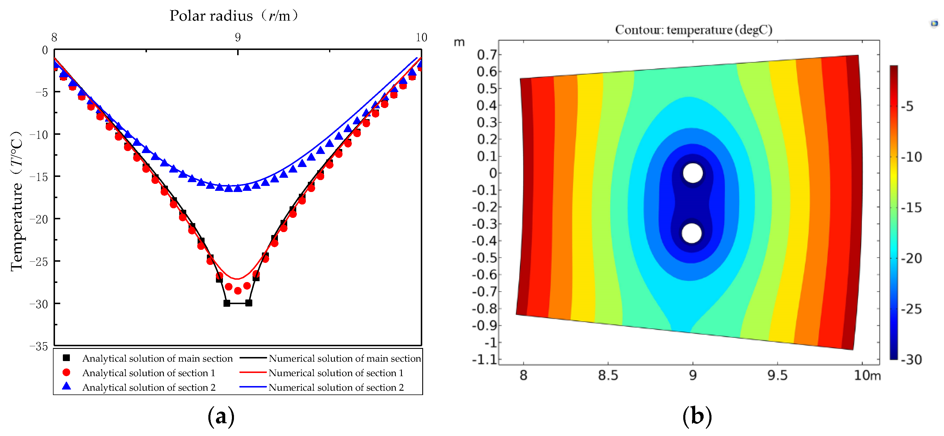
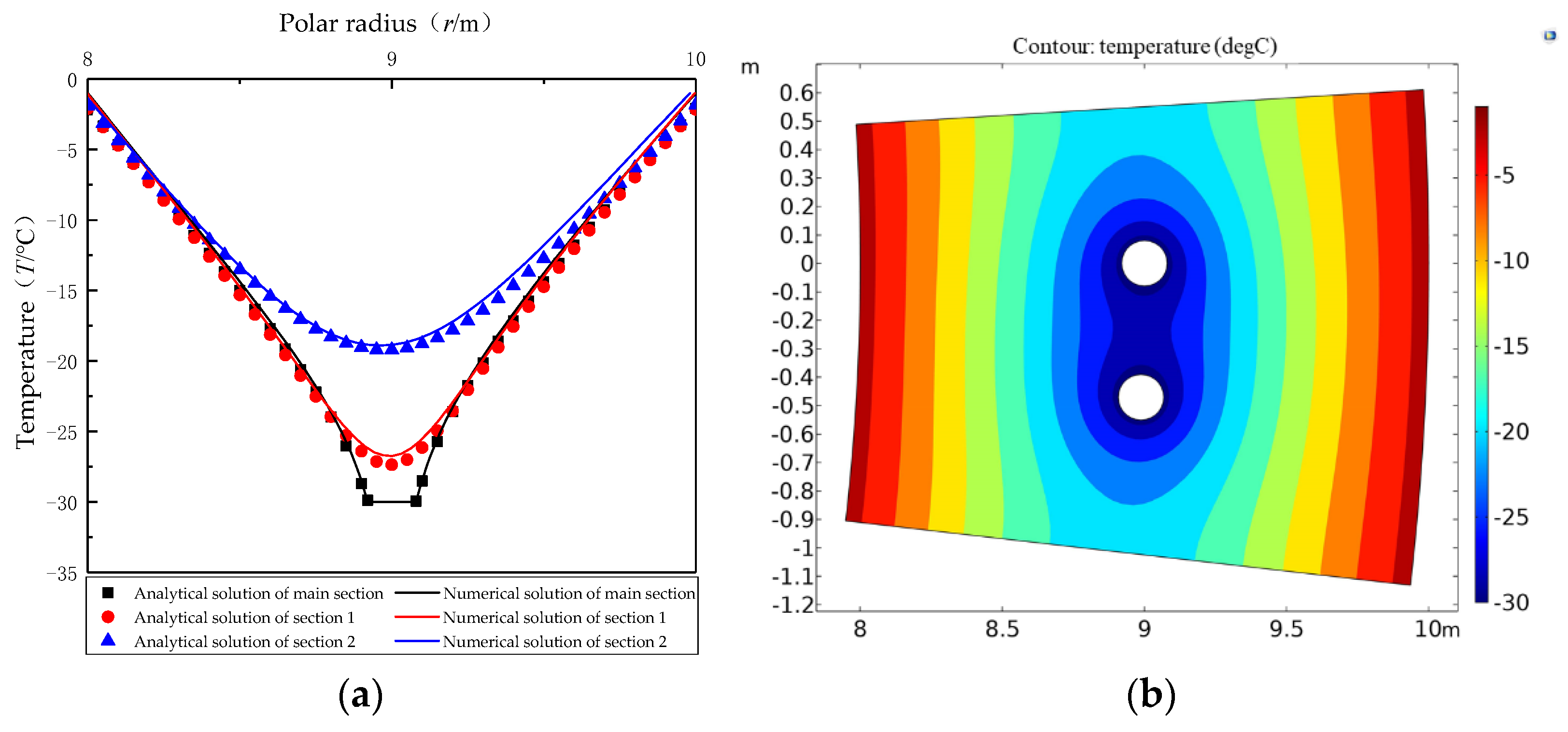
3.3. Comparative Analysis of Calculation Results

Calculation results and the cloud map of the temperature field are compared as shown in Figure 8, Figure 9, Figure 10, Figure 11, Figure 12 and Figure 13:

From Figure 8, Figure 9, Figure 10, Figure 11, Figure 12 and Figure 13, the analytical solution and numerical solution curve for each model section under six groups of different parameters coincide, and maximum temperature differences at each point do not exceed 0.9 °C. The data indicate that the steady-state temperature field model of the complicated freezing tube layout in FSPR can be simplified, and conformal mapping and the separation-variable method can be employed to solve the problem. The derived analytical solution is highly accurate, and can accurately calculate the temperature value at any point in the model.

In the vicinity of the inner and outer boundaries of the model’s frozen soil, temperatures of the three sections in each group are relatively close, corresponding to symmetrical and uniform temperature distributions on both sides of steady-state temperature field cloud map. In the area closer to the freezing tube, temperature differences among the three sections are greater, and the maximum temperature difference is located at the axial surface R₂ of the freezing tube. The temperature curve of Section 1 is located between Section 2 and the main section, and is closer to the latter.

In actual engineering, Section 1 is the position of the midline between the adjacent concrete pipe and hollow pipe, and is an important area for “freeze-sealing between pipes” in FSPR. The above figures show that the temperature range of this area within the size range of the pipe is −10 °C~−28 °C and the distribution is relatively uniform, implying that a reliable frozen soil curtain can be formed between the jacking pipes to ensure “freeze-sealing” effects and safety.

3.4. Discussion of Analytical Solution in FSPR

From the parameter selection of each group in Table 1, the smaller the dislocation angle β value and the larger the frozen tube radius R₀, the lower the temperature of the freezing tube area. In the FSPR method adopted in the Gongbei Tunnel, the approximate circle radius of the freezing tube ring is about 9 m, and the diameter of the jacking pipe is 1.62 m. The distance between adjacent jacking pipes is about 0.3 m, and the dislocation angle is about 2°. Taking the freezing parameters R₁ = 7.9 m, R₂ = 9 m, R₃ = 10 m, and ξ₁/ξ₂ = 1.1 at the end of the freezing stage, respectively, calculate the temperature difference of the three sections of the frozen soil curtain at the axial surface R₂ of the freezing tube, as shown in

Table 2. Temperature differences of each section at the end of freezing.

	Main Section	Section 1	Section 2
Temperature/°C	−30	−28.51	−16.08
ΔT1/°C	−1.49		——
ΔT2/°C	——	−12.43

:

At the end of freezing, the temperature difference between the main section and Section 1 is ΔT1 = −1.49 °C, while the temperature difference between sections 1 and 2 is ΔT2 = −12.43 °C. Section 2 is located at the axis of symmetry of the steel jacking pipe, which can provide effective water sealing capacity, therefore, only Section 1 should be considered. The temperature for Section 1 can drop to a lower temperature value at the end, which is very close to the temperature of the freezing tubes in the main section. Notably, frozen soils can be formed with sufficient strength and water sealing performance between the jacking pipes. Then, an effective frozen curtain is formed as a whole, which provides safe and reliable support for tunnel excavation.

Finally, the steady-state temperature field distribution cloud map of the overall model in FSPR is calculated and drawn in line with the analytical solution formula, (Figure 14). The analytical solution obtained in this article has sufficient accuracy to meet the calculation needs of different positions (pole radius r) in the FSPR model. The temperature field cloud map, drawn according to the calculation results, can intuitively reveal the overall temperature distribution and thickness of the frozen soil curtain, and realize visual processing. It is also proven that when the temperature field tends to steady-state in the latter stage of freezing, the shapes of the inner and outer boundaries of the frozen soil in this model can be considered to be a circular ring, and the wavy frozen soil boundary can be ignored.

4. Conclusions

(1)

During the freezing process of FSPR, formation of the frozen curtain is largely dependent on two types of freezing tubes to freeze the soil between the jacking pipes, and achieve the purpose of sealing water. Taking this as the main research object of the freezing steady-state temperature field, the model is assumed and simplified in combination with actual situation of the Gongbei tunnel project. Using the conformal mapping function and the separation-variable solution method, the analytical solution expression for the steady-state temperature field of FSPR under different soil freezing points is deduced, which is a quick calculation method that can be used by engineers and technicians during the designing stage and to evaluate the effect of on-site freezing construction.

(2)

Different characteristic parameters and finite element software can be used to establish and solve the corresponding two-dimensional steady-state temperature field numerical calculation model. The correctness and accuracy of the analytical solution are verified by comparing the results. In this project, the calculation result is acceptable when the soil freezing point range is 0~−1.5 °C.

(3)

Combined with the contour map of the steady-state temperature field, it is shown that when the number of frozen tubes is large, that is, the spacing between the freezing tubes is small, the shapes of the inner and outer boundaries of the frozen soil curtain can be approximately regarded as circular rings in the steady state.

(4)

The temperature difference of the three sections is larger in the region closer to the freezing tube. Section 1 is the position of the midline between the adjacent concrete pipe and hollow pipe, and is an important area for “freeze-sealing between pipes” in FSPR. The calculated results show that the temperature range of this area within the size range of the pipe is −10 °C~−28 °C, implying that a reliable frozen soil curtain can be formed between the jacking pipes to ensure the effect of “freeze-sealing” and safety.

(5)

How to adapt the analytical solution of temperature field to the operating state of various frozen tubes is a problem that requires further investigation. In addition, the actual tunnel section is closer to that of the ellipse, and considering these conditions, the analytical solution also deserves further exploration.

References

1. Cheng, X.S. Ground Freezing Method, 1st ed.; China Communications Press: Beijing, China, 2013; pp. 3–4. (In Chinese) [Google Scholar]
2. Cheng, H. Theory and Technology of Shaft Sinking by Freezing Method for Deep Alluvium, 1st ed.; Science Press: Beijing, China, 2016; pp. 118–120. (In Chinese) [Google Scholar]
3. Wang, B.; Rong, C.X.; Cheng, H. Analytical Solution of Steady-state Temperature Field of Asymmetric Frozen Wall Induced by Directional Seepage. Adv. Eng. Sci. 2022, 54, 76–87. [Google Scholar] [CrossRef]
4. Taylor, R.N. Geotechnical Centrifuge Technology, 1st ed.; Blackie Academic & Professional: London, UK, 1994; pp. 273–280. [Google Scholar]
5. Cai, H.B.; Li, S.; Liang, Y.; Cheng, H. Model Test and Numerical Simulation of Frost Heave During Twin-tunnel Construction using Artificial Ground-freezing Technique. Comput. Geotech. 2019, 115, 103155. [Google Scholar] [CrossRef]
6. Huang, X.W.; Yao, Z.S.; Cai, H.B.; Li, X.; Chen, H. Performance evaluation of coaxial borehole heat exchangers considering ground non-uniformity based on analytical solutions. Int. J. Therm. Sci. 2021, 170, 107162. [Google Scholar] [CrossRef]
7. Li, K.Q.; Li, D.Q.; Liu, Y. Meso-scale investigations on the effective thermal conductivity of multi-phase materials using the finite element method. Int. J. Heat Mass Transf. 2020, 151, 119383. [Google Scholar] [CrossRef]
8. Hosseini, S.M.; Akhlaghi, M.; Shakeri, M. Transient Heat Conduction in Functionally Graded Thick Hollow Cylinders by Analytical Method. Heat Mass Transf. 2007, 43, 669–675. [Google Scholar] [CrossRef]
9. Jiang, B.S.; Shen, C.R.; Feng, Q. Analytical Formulation of Temperature Field of Single Freezing Pipe with Constant Outer Surface Temperature. J. China Coal Soc. 2010, 35, 923–927. [Google Scholar] [CrossRef]
10. Cai, H.B.; Xu, L.X.; Yang, Y.G.; Li, L. Analytical Solution and Numerical Simulation of the Liquid Nitrogen Freezing Temperature Field of a Single Pipe. AIP Adv. 2018, 8, 055119. [Google Scholar] [CrossRef] [Green Version]
11. Fang, T.; Hu, X.D. Generalized Analytical Solution to Steady-state Temperature Field of Single-row-piped Freezing. J. China Coal Soc. 2019, 44, 535–543. [Google Scholar] [CrossRef]
12. Sanger, F.J.; Sayles, F.H. Thermal and Rheological Computations for Artificially Frozen Ground Construction. Eng. Geol. 1979, 13, 311–337. [Google Scholar] [CrossRef]
13. Trupak, N.G. Groud Freezing in Shaft Sinking; Coal Technology Press: Moscow, Russia, 1954; pp. 20–65. (In Russian) [Google Scholar]
14. Bakholdin, B.V. Selection of Optimized Mode of Ground Freezing for Construction Purpose; State Construction Press: Moscow, Russia, 1963; pp. 21–27. (In Russian) [Google Scholar]
15. Hu, C.P.; Hu, X.D.; Zhu, H.H. Sensitivity Analysis of Control Parameters of Bakholdin Solution in Single-row-pipe Freezing. J. China Coal Soc. 2011, 36, 938–944. [Google Scholar] [CrossRef]
16. Yang, B.; Ding, W.Q.; Hu, X.D.; Liu, P. Sensitivity Analysis of Control Parameters for Average Temperature of Single-Row-Pipe Frozen Soil Wall. Chin. J. Undergr. Space Eng. 2012, 8, 1208–1214. [Google Scholar]
17. Hu, X.D.; Zhang, L.Y. Analytical Solution to Steady-State Temperature Field of Two Freezing Pipes with Diferent Temperatures. J. Shanghai Jiaotong Univ. (Sci.) 2013, 18, 706–711. [Google Scholar] [CrossRef]
18. Hu, X.D.; Han, Y.G.; Yu, X.F. Generalized Analytical Solution to Steady-state Temperature Field of Double-row-pipe Freezing. J. Tongji Univ. (Nat. Sci.) 2015, 43, 386–391. [Google Scholar] [CrossRef]
19. Hu, X.D.; Wang, Y. Analytical Solution of Three-row-piped Frozen Temperature Field by Means of Superposition of Potential Function. Chin. J. Rock Mech. Eng. 2012, 31, 1071–1080. [Google Scholar] [CrossRef]
20. Wang, B.; Rong, C.X.; Cheng, H. Elastic and Plastic Analysis of Heterogeneous Frozen Soil Wall of Triple-row Piped Freezing. J. Yangtze River Sci. Res. Inst. 2019, 36, 104–111. [Google Scholar] [CrossRef]
21. Hu, X.D.; Han, Y.G. General Analytical Solution to Steady-state Temperature Field of Single-circle-pipe Freezing. J. Cent. South Univ. (Sci. Technol.) 2015, 46, 2342–2349. [Google Scholar] [CrossRef]
22. Hu, X.D.; Fang, T.; Han, Y.G. Generalized Analytical Solution to Steady-state Temperature Field of Double-circle-piped Freezing. J. China Coal Soc. 2017, 42, 2287–2294. [Google Scholar] [CrossRef]
23. Hu, X.D.; Huang, F.; Bai, N. Models of Artificial Frozen Temperature Field Considering Soil Freezing Point. J. China Univ. Min. Technol. 2008, 37, 550–555. [Google Scholar]
24. Hong, Z.Q.; Shi, R.J.; Yue, F.T.; Han, L. Analytical Solution of Steady-state Temperature Field for Large-section Freezing with Rectangular Layout of Single-ring holes. Chin. J. Geotech. Eng. 2022, 9, 1–10. Available online: https://kns.cnki.net/kcms/detail/32.1124.TU.20220922.0943.006.html (accessed on 23 September 2022).
25. Qi, Y.; Zhang, J.; Yang, H.; Song, Y. Application of Artificial Ground Freezing Technology in Modern Urban Underground Engineering. Adv. Mater. Sci. Eng. 2020, 2020, 1619721. [Google Scholar] [CrossRef]
26. Liu, J.G.; Ma, B.S.; Cheng, Y. Design of the Gongbei Tunnel Using a Very Large Cross-section Pipe-roof and Soil Freezing Method. Tunn. Undergr. Space Technol. 2018, 72, 28–40. [Google Scholar] [CrossRef]
27. Kang, Y.S.; Liu, Q.S.; Cheng, Y.; Liu, X. Combined Freeze-sealing and New Tubular Roof Construction Methods for Seaside Urban Tunnel in Soft Ground. Tunn. Undergr. Space Technol. 2016, 58, 1–10. [Google Scholar] [CrossRef]
28. Zhang, D.M.; Pang, J.; Ren, H.; Han, L. Observed Deformation Behavior of Gongbei Tunnel of Hong Kong-Zhuhai-Macao Bridge During Construction. Chin. J. Geotech. Eng. 2020, 42, 1632–1641. [Google Scholar] [CrossRef]
29. Long, W.; Rong, C.X.; Duan, Y.; Guo, K. Numerical Calculation of Temperature Field of Freeze-sealing Pipe Roof Method in Gongbei Tunnel. Coal Geol. Explor. 2020, 48, 160–168. [Google Scholar] [CrossRef]
30. Hu, X.D.; Li, X.Y.; Wu, Y.H.; Han, L.; Zhang, C.B. Effect of Water-proofing in Gongbei Tunnel by Freeze-sealing Pipe Roof Method with Field Temperature Data. Chin. J. Geotech. Eng. 2019, 41, 2207–2214. [Google Scholar] [CrossRef]
31. Guo, K.; Duan, Y. Numerical Simulation of Temperature Field of Tube-Curtain Freezing Method for Shallow Buried Tunnel. J. Anhui Univ. Sci. Technol. (Nat. Sci.) 2019, 39, 63–68. [Google Scholar]
32. Hu, X.D.; Hong, Z.Q.; Fang, T. Analytical Solution to Steady-state Temperature Field with Typical Freezing Tube Layout Employed in Freeze-sealing Pipe Roof Method. Tunn. Undergr. Space Technol. 2018, 79, 336–345. [Google Scholar] [CrossRef]
33. Kong, X.Y. Advanced Mechanics of Fluids in Porous Media, 3rd ed.; USTC Press: Hefei, China, 2020; pp. 84–90. (In Chinese) [Google Scholar]
34. Li, H.; Xie, S.F. Complex Variable Function & Integral Transform, 5th ed.; Higher Education Press: Beijing, China, 2018; pp. 155–164. (In Chinese) [Google Scholar]
35. Wang, R.H.; Li, X.J. Superposition Calculation of Frozen Temperature Field and Its Computer Method. J. Anhui Univ. Sci. Technol. (Nat. Sci.) 2003, 1, 25–29. [Google Scholar] [CrossRef]
36. Hu, X.D.; Guo, W.; Zhang, L.Y. Mathematical Models of Steady-state Temperature Fields Produced by Multipiped Freezing. J. Zhejiang Univ.-SCIENCE A (Appl. Phys. Eng.) 2016, 17, 702–723. [Google Scholar] [CrossRef]
37. Chen, S.X.; Qin, T.H.; Zhou, Y. Mathematical Physics Equation, 1st ed.; Fudan University Press: Shanghai, China, 2003; pp. 61–63. (In Chinese) [Google Scholar]
38. COMSOL Multiphysics Reference Manual. 2018. Available online: https://doc.comsol.com/5.4/doc/com.comsol.help.comsol/COMSOL_ReferenceManual.pdf (accessed on 19 October 2022).
Figure 1. Schematic presentation of FSPR applied in the Gongbei Tunnel.
Applsci 12 11576 g001
Figure 2. Layout of pipe roof and freezing tube in Gongbei Tunnel.
Applsci 12 11576 g002
Figure 3. Simplified model of freezing temperature field of FSPR.
Applsci 12 11576 g003
Figure 4. Freezing temperature field model in image plane of non-equidistant single-row tube with asymmetric development of frozen curtain.
Applsci 12 11576 g004
Figure 5. Freezing temperature field model in image plane of two kinds of linear single-row tubes: (a) A′-type linear single-row tube; (b) B′-type linear single-row tube.
Applsci 12 11576 g005
Figure 6. Computational periodic element model of the analytical solution.
Applsci 12 11576 g006
Figure 7. Numerical model of parameter group 1: (a) Model; (b) Computational domain grid.
Applsci 12 11576 g007
Figure 8. Comparison of the 1st group of calculation results: (a) Comparison curve between analytical and numerical solutions of section; (b) Steady-state temperature field.
Applsci 12 11576 g008
Figure 9. Comparison of the 2nd group of calculation results: (a) Comparison curve between analytical and numerical solutions of section; (b) Steady-state temperature field.
Applsci 12 11576 g009
Figure 10. Comparison of the 3rd group of calculation results: (a) Comparison curve between analytical and numerical solutions of section; (b) Steady-state temperature field.
Applsci 12 11576 g010
Figure 11. Comparison of the 4th group of calculation results: (a) Comparison curve between analytical and numerical solutions of section; (b) Steady-state temperature field.
Applsci 12 11576 g011
Figure 12. Comparison of the 5th group of calculation results: (a) Comparison curve between analytical and numerical solutions of section; (b) Steady-state temperature field.
Applsci 12 11576 g012
Figure 13. Comparison of the 6th group of calculation results: (a) Comparison curve between analytical and numerical solutions of section; (b) Steady-state temperature field.
Applsci 12 11576 g013
Figure 14. Two-dimensional steady-state temperature field based on analytical solution.
Applsci 12 11576 g014