A Model of a Limited-Stop and Local Mixed Bus Service with Increased Fares for the Limited-Stop Service

Abstract

This study designs a limited-stop and local mixed bus service from the perspectives of both transit agencies and passengers based on a proposed optimization model. Close attention was paid to the increase in fares for the limited-stop service in the proposed model to offset the loss in bus fare. The objective function was to minimize the passenger travel time and bus agency costs; the decision variables were the stops for the limited-stop service and the headways of the limited-stop and local services; the constraints included the range of fare increases for the limited-stop service and other factors. The Lingo software and the genetic algorithm were compared in solving the proposed model from the aspects of solving time and results. Because the solutions for the model within the planning time and the influence of the global optimal solution upon parametric analysis were stable, the Lingo software was more suitable for the proposed model. Evaluations of the total costs for the mixed service and local-only service were carried out for different bus corridor lengths. The ratio of the fares for the limited-stop service to the fares for the local service must be within the appropriate range in order to take advantage of the limited-stop service. When the stop spacing and the bus corridor distance were longer, the mixed service was more competitive and noticeable.

1. Introduction

Increasing sharing of buses can relieve traffic congestion and reduce the emission of pollution. The strategy for designing a bus affects the efficiency of the bus and the design of bus stops, which play a pivotal role in the level of bus service. To make full use of bus resources, fixed bus routes naturally become many types of bus routes, based on whether they are stop services. These types include local, limited-stop, express, semi-restricted zonal service, restricted zonal service, short-turning, and deadheading [1]. Bogota, Los Angeles [2], Santiago [3], Jinan [4], Guangzhou [5], Montréal [6], and many other cities have applied various types of bus routes to make full use of public transportation.

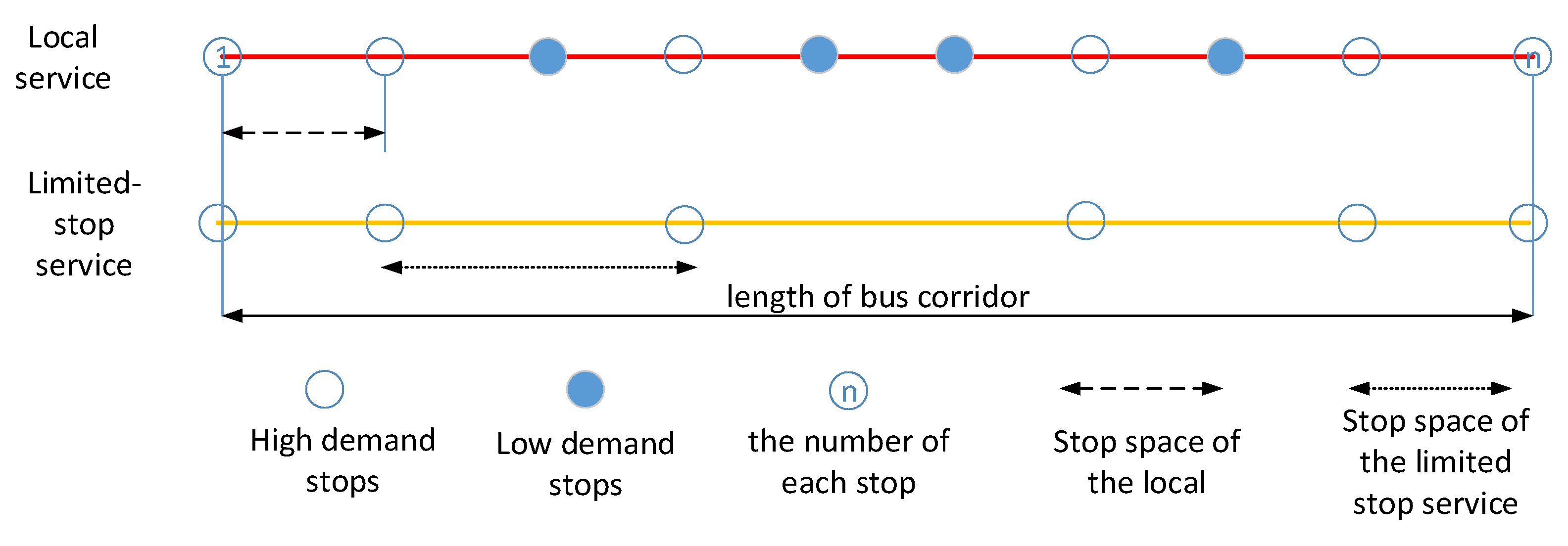
A local service provides services at all stops along the route, with accessibility being more important. Vehicles used for limited-stop services only stop at high-demand stops; thus, speed and accessibility are relatively balanced. Limited-stop service can shorten the in-vehicle travel time of the serviced passengers [6] and improve the utilization of bus resources [7], whereas the access or egress time and waiting time for limited-stop service for some passengers will increase. Limited-stop services usually operate in a long bus corridor with a long bus route. The passenger demand along the bus corridor is usually high, and the distribution is unbalanced. Limited-stop services can be beneficial to both bus agencies and passengers under appropriate conditions. For bus agencies, the shorter operating cycle of limited-stop service increases bus vehicle utilization, improving the capacity and operational efficiency. In addition, operating costs are reduced due to lower passenger boarding and alighting times. Limited-stop service is also attractive to passengers, by providing faster trips for some origin–destination (OD) pairs, especially for passengers with long commuting distances. Mixed service of local and limited stops can balance the advantages of both types, which are shown in Figure 1.

At present, some bus stop design models are used as express services [8,9,10]. Several researchers have studied the design of limited-stop services in different situations. Chen et al. [11] and Soto [12] focused on the dynamics of demand, and the results showed that flexible passenger trips would make better use of the limited-stop service. Compared with the previous literature, Chiraphadhanakul [13] considered the constraints of the fleet and redistributed the existing vehicles instead of adding vehicles to the limited-stop service. To expand a limited-stop service to a whole bus network, Leiva et al. [14] considered transfers of the limited-stop design. Evaluation of the limited-stop service was also a focus. Customer satisfaction is one of the main ways to measure the performance of limited-stop services [15,16,17]. To overcome the limitations of the importance of performance analysis, Wu et al. [18] proposed a three-factor theory based on existing factors, important factors, and basic factors to analyze a limited-stop service’s performance. Different from the satisfaction survey, Geneidy et al. [19] evaluated the newly implemented limited-stop service on Montreal Island, Canada. They collected vehicle location and passenger trip data to compare the on-time rate of the vehicles before and after the implementation of the service.

The fare is an essential factor for both bus agencies and passengers in a limited-stop service. If the subsidy from the government remains unchanged and the fare for the limited-stop service is also the same as that for the local service, then the bus agency will have a deficit in their mixed-service operations. Differentiated fares are a gainful way to compensate for the reduction in fare revenue for bus agencies caused by the decreasing number of passengers due to the implementation of limited-stop services. In the current literature, differentiated fares for a limited-stop service and a local service have been insufficiently considered. In this study, special attention was paid to the increase in the fare for a limited-stop service. The distance of a bus corridor is also critical. The number of stops and average stop spacing commonly determine the distance of bus corridors. Mixed services operating within unreasonable conditions can lead to poor public transportation service quality. The number of vehicles in the mixed service does not increase in many routes. So, the waiting time for local service passengers increases, and the reduced in-vehicle time for limited-stop service passengers may be offset by increased waiting time. For the mixed service system, the total passenger travel time increases instead. The current literature on the evaluation of bus service efficiency has been mostly based on supervisory factors such as passenger perception. In most studies in the literature, the mixed service design problems were solved through heuristic methods that could not obtain global optimal solutions. Without access to a global optimal solution, the analysis of critical factors in the system cannot be carried out. Very few studies have focused on the impact of a bus corridor’s distance on the performance of limited-stop and local services.

In this paper, a limited-stop and local mixed-service model was proposed to minimize the total cost, combining the characteristics of fast speed of limited-stop and good accessibility of local. The increased fare for the limited-stop service was introduced into the model. The contributions of this study include: (1) The increased fare for the limited-stop service was proposed for the first time. Through case studies, we analyzed the effects of increased fare on the objective function and decision variables, and determined the range of increased fare. For the limited-stop operators, the increased fare improves the incentive to operate limited-stop services and avoids the decline in wages for drivers and revenues for individual operators of limited-stop services due to the decline in limited-stop passengers; according to the questionnaire survey, passengers could accept the increase in fare within a reasonable range to enjoy faster service. (2) The conditions for application of mixed limited-stop and local services were determined, combined with the parameters such as the number of bus stops and the average stop spacing. The achievements were conducive to improving the service quality of mixed services and avoiding the increase in “door to door” travel time for all passengers due to improperly designed mixed services. (3) From the algorithmic point of view, it was verified that the model of the limited-stop service and local mixed service was more suitable to be solved by Lingo software relative to the genetic algorithm. Solving the mixed service model by Lingo not only reduced the total cost, but also the global optimal solution obtained could be used to analyze the impact of fare and the conditions for application of the mixed service.

The rest of the paper is organized as follows: Section 2 describes the proposed model, a mixed limited-stop and local bus service, along with the decision variables, objective function, and constraints. Section 3 analyzes the feasibility of the proposed model for the study case of Jinan, China. The Lingo software and the genetic algorithm were compared for the proposed model, with the results showing that the Lingo software program was better. Section 4 discusses the impacts of increasing the fare on the limited-stop service, the bus corridor’s distance on the competitiveness of the mixed-service and local-only service, as well as the impacts under different hyper-parametrizations. Section 5 provides the conclusions and considerations of the paper.

2. Model

The limited-stop and local mixed bus service proposed in this paper is suitable for operating along bus corridors between different cities and regional areas, especially for commuters whose origins and destinations are in different urban areas. By removing some of the stops, the cycle time is reduced and the travel speed of limited-stop service is improved. It not only improves the level of service for passengers, but it also makes it more cost-effective for the bus agency.

The limited-stop bus service has the ability to serve a market of passenger demand that falls between regional express and local bus operations. A long bus corridor with an uneven distribution of travel demand is better for running a limited-stop service. The limited-stop service can take full advantage of its balanced speed and accessibility features and reduce the “door-to-door” time for commuters.

The proposed model’s objective was to minimize the system’s cost, including the agency cost and passenger cost. It was assumed that the weights of the agency cost and passenger cost were the same, as in Daganzo [20]. The limited-stop service stops can be chosen based on unbalanced passenger travel demand caused by different origin and destination demands within each stop. The number of local vehicles and limited-stop vehicles are determined by the respective headways. Therefore, the decision variables included the headway of the limited-stop service (H_e), the stops for the limited-stop service headway of the local service (H_L), and the stops for the limited-stop service (x_i). The parameters are listed in Appendix A.

2.1. Agency Cost

The agency cost consists of the total distance traveled by the vehicles per hour and the total number of vehicles per hour. The local service and limited-stop service costs were calculated separately; thus, the agency costs could be divided into two types. From this, the following was obtained.

$$M_L=\frac{2L}{H_L{v}_c{}_L}$$

(1)

$$M_e=\frac{2L}{H_e{v}_{ce}}$$

(2)

$$V_L=M_L·v_{cL}$$

(3)

$$V_e=M_e·v_{ce}$$

(4)

$$\raisebox{1ex}{$1$}\!\left/ \!\raisebox{-1ex}{$v_c{}_L$}\right.\approx 1/v+\tau /\overline{s}+{\tau }^{\prime }{P}_L/L$$

(5)

$$\raisebox{1ex}{$1$}\!\left/ \!\raisebox{-1ex}{$v_{ce}$}\right.\approx 1/v+\tau /\overline{s_e}+{\tau }^{\prime }{P}_e/L$$

(6)

Equations (1) and (2) are the number of local vehicles and limited-stop vehicles operating on the two-way line per hour, respectively; the number of vehicles operating on the one-way line is equal to the ratio of the bus line to the product of the travel speed and headway, while the number of vehicles operating on the two-way line is twice the number of vehicles operating on the one-way line [20].

Equations (3) and (4) are the total distances traveled by the vehicles per hour for both types of services, which are the product of the travel speed and the number of vehicles per hour [20].

Equations (5) and (6) aim to calculate the travel speed of the two types of services; the travel speed is the ratio of the bus line’s length to the travel time. The travel time (L/v_c) was composed of three parts: the driving time (L/v), lost time at a stop ($\tau n$), and the boarding and alighting time of passengers (${\tau }^{\prime }{P}_e$ or ${\tau }^{\prime }{P}_L$).

2.2. Passenger Cost

The travel time generally includes the transfer time, access and egress times, waiting time, and in-vehicle time of the passengers. Access time is the time from the origin to the passenger get-on stop, and egress time is the time from the passenger drop-off stop to the destination. Access and egress times can be viewed as one parameter [20]. Here, only one bus corridor was considered without transfer; therefore, the passenger cost only included the last three. The increased fare for the limited-stop service was proposed in the model. The fare for the limited-stop service increases to avoid a decline in fare revenue for individual operators and wages for drivers of limited-stop service caused by the reduction in passengers. Many buses drivers’ performance pay is based on passenger fare revenue. According to the questionnaire survey, passengers could accept the increase in fare within a reasonable range to enjoy faster service.

Based on whether the origin and destination stops of a passenger were serviced by a limited-stop vehicle, passengers were divided into three types: (1) both the origin and destination stops were serviced by limited-stop vehicles; (2) only the origin stop was serviced by limited-stop vehicles; (3) neither the origin stop nor the destination stop was serviced by limited-stop vehicles. Passengers whose only destination stop was serviced by a limited-stop vehicle were also viewed as type (3).

According to the above classification, the following conclusions can be obtained. Passengers categorized as types (1) and (2) can choose both services. For passengers belonging to type (1), the egress time is the same whether they choose a limited-stop or a local service, while if passengers of type (2) choose the limited-stop service instead of the local service, they will require an additional egress distance that is equal to a one-stop spacing distance due to the original destination stop not being served by a limited-stop vehicle. Passengers of type (3) will only travel by local service [21]. All three passenger types can choose to travel by a local vehicle. The assumptions were as follows:

• Limited-stop services only operate in peak hours.
• Passengers of type (1) and type (2) will choose the first-coming bus, regardless of the service type [22]. Although the limited-stop fare is more expensive, the increasing fare can be accepted by passengers within a suitable range, and the time value for passengers during peak hours is still much higher. For the same reason, during peak hours, passengers will not consider the congestion in the vehicles;
• Passengers can accept a higher fare for the limited-stop service within a reasonable interval. A reasonable interval can be obtained by a willingness survey. Bus companies can realize the difference in fares through an IC card or APPS of the bus company;
• Passengers between two nearby stops are evenly distributed in the one-bus-stop spacing;
• The OD matrix, P, and the stop distance matrix, D, between stops are known;
• The limited-stop service only has a one-stop pattern, and the stops along the uplink and downlink lines of the limited-stop service are consistent, which is favorable for limited-stop passengers;
• To improve the utilization of bus services, the mixed service operates during peak hours [23], while in off-peak hours, the bus agency only provides local service.

$$P_e=\frac{\frac{1}{H_e}}{\frac{1}{H_L}+\frac{1}{H_e}}(P_{total}-{\displaystyle \sum _{i=1}^n(1-x_i){\displaystyle \sum _{j=1}^n{p}_{ij}})}$$

(7)

$$P_L=P_{total}-P_e$$

(8)

$$P_{ee}=\frac{\frac{1}{H_e}}{\frac{1}{H_L}+\frac{1}{H_e}}({\displaystyle \sum _{i=1}^n{\displaystyle \sum _{j=1}^n{x}_i{x}_j{p}_{ij}}})$$

(9)

$$P_{eL}=P_e-P_{ee}$$

(10)

$$W_L=\frac{H_L}{2}$$

(11)

$$W_e=\frac{H_e}{2}$$

(12)

$$A_{ee}=A_L=\frac{\overline{s}}{v_w}$$

(13)

$$A_{eL}=\frac{2\overline{s}}{v_w}$$

(14)

$$T_L=\frac{{\overline{D}}_L}{v_{cL}}=\frac{{\displaystyle \sum _{i=1}^n{\displaystyle \sum _{j=1}^n(1-x_i)p_{ij}}{d}_{ij}}+\frac{\frac{1}{H_L}}{\frac{1}{H_L}+\frac{1}{H_e}}({\displaystyle \sum _{i=1}^n{\displaystyle \sum _{j=1}^n{p}_{ij}{d}_{ij}}}-{\displaystyle \sum _{i=1}^n{\displaystyle \sum _{j=1}^n(1-x_i)p_{ij}{d}_{ij}})}}{\left[{\displaystyle \sum _{i=1}^n{\displaystyle \sum _{j=1}^n(1-x_i)p_{ij}}}+\frac{\frac{1}{H_L}}{\frac{1}{H_L}+\frac{1}{H_e}}({\displaystyle \sum _{i=1}^n{\displaystyle \sum _{j=1}^n{p}_{ij}}}-{\displaystyle \sum _{i=1}^n{\displaystyle \sum _{j=1}^n(1-x_i)p_{ij})}}\right]v_{cL}}$$

(15)

$$T_{ee}=\frac{{\overline{D}}_{ee}}{v_c{}_e}=\frac{{\displaystyle \sum _{i=1}^n{\displaystyle \sum _{j=1}^n{x}_i{x}_j{p}_{ij}}}·d_{ij}}{\left({\displaystyle \sum _{i=1}^n{\displaystyle \sum _{j=1}^n{x}_i{x}_j{p}_{ij}}}\right)v_{ce}}$$

(16)

$$T_e{}_L=\frac{{\overline{D}}_{eL}}{v_c{}_e}=\frac{{\displaystyle \sum _{i=1}^n{\displaystyle \sum _{j=1}^n{x}_i(1-x_j)p_{ij}}}·d_{ij}}{\left[{\displaystyle \sum _{i=1}^n{\displaystyle \sum _{j=1}^n{x}_i(1-x_j)p_{ij}}}\right]v_{ce}}$$

(17)

Equations (7)–(10) are the total number of the different types of passengers. The number of passengers using the limited-stop service is the product of the total number of passengers of type (1) and type (2) and the probability that the limited-stop vehicle will arrive first; $(P_{total}-{\displaystyle \sum _{i=1}^n(1-x_i){\displaystyle \sum _{j=1}^n{p}_{ij}})}$ is the total number of type (1) and type (2) passengers; $\frac{\frac{1}{H_e}}{\frac{1}{H_L}+\frac{1}{H_e}}$ is the probability that the limited-stop vehicle will arrive first. The total number of passengers using the local service is equal to the total number of passengers minus the total number of passengers for the limited-stop service. The method for calculating P_ee is the same as that for calculating P_e.

Equations (11) and (12) are the waiting times, which are half the headways of the available vehicles [20].

Equations (13) and (14) are the access and egress times. For passengers, the maximum distance travelled at each end is s, and the average is 1/2 s; therefore, the total walking distance around the origin stop to the destination stop is s. Limited-stop passengers of type (2) need an additional egress distance equal to a one-stop spacing distance.

Equations (15)–(17) are the in-vehicle times; the in-vehicle time of each service is the ratio of the average travel distance to the travel speed. The average travel distance is the ratio of the total travel distance to the number of passengers; the calculation of the total travel distance is performed using P and D.

2.3. Objective Function

The objective function given by Equation (18) consists of three parts: the first bracket denotes the cost for local passengers, the second bracket denotes the cost for limited-stop passengers of type (1), and the last one denotes the cost for limited-stop passengers of type (2). Each part has two kinds of costs: the agency cost and the passenger cost. The unit of measurement for the agency cost and the passenger cost is not uniform; thus, according to the findings by Daganzo [20], the agency cost was converted into time. Therefore, V and M are multiplied by the weight, ${\mathsf{\pi }}_V{=\text{\$}}_V/(\lambda \mu )$, and ${\mathsf{\pi }}_M{=\text{\$}}_M/(\lambda \mu )$. For the passenger cost, A and W are multiplied by the weights w_A and w_w, respectively. The constraints are given by Equations (19)–(24).

$$\begin{array}{l}\min C=P_L·[{\mathsf{\pi }}_V{V}_L+{\mathsf{\pi }}_M{M}_L+w_A{A}_L+w_w{W}_L+T_L]+\\ P_{ee}·[({\mathsf{\pi }}_V{V}_e+{\mathsf{\pi }}_M{M}_e)\frac{P_{ee}}{P_{total}}+w_A{A}_{ee}+w_w{W}_e+T_{ee}]\\ +P_{eL}·[({\mathsf{\pi }}_V{V}_e+{\mathsf{\pi }}_M{M}_e)\frac{P_{eL}}{P_{total}}+w_A{A}_{{}_{eL}}+w_w{W}_e+T_{eL}]\end{array}$$

(18)

$$H_L>2$$

(19)

$$H_e>2$$

(20)

$$M_L+M_e\le M,M\in N^{*},M_L\in N^{*},M_e\in N^{*}$$

(21)

$$({\mathsf{\pi }}_V{V}_e+{\mathsf{\pi }}_M{M}_e)\frac{P_{total}}{P_e}\le g({\mathsf{\pi }}_V{V}_L+{\mathsf{\pi }}_M{M}_L)$$

(22)

$$0\le x_i\le 1,x_i\in N^{*} (i=1, 2,\cdots , n)$$

(23)

$$x_i+x_{i-1}+x_{i-2}\ge 1 (i=3, 4,\cdots , n)$$

(24)

$$\max \{\frac{P_L}{M_L},\frac{Pe}{Me}\}\le Z$$

(25)

The headways of the limited-stop service and the local service are more than 2 min to avoid bus bunching of the same kind of service, as under the constraints in Equations (19) and (20) [20,24]. During the mixed service, vehicle overtaking is allowed in order to decrease the system costs [5]. Equation (21) restricts the vehicle fleet in the mixed service so that the number of vehicles is unchanged instead of adding vehicles to the limited-stop service. Equation (22) limits the range of the fare increase for the limited-stop service. For bus agencies, the deficit caused by decreasing passengers can be avoided. At the same time, the increased fare can be accepted by the passengers. In Equation (23), if stop i is serviced by a limited-stop vehicle, x_i is 1, else x_i is 0. The additional egressing distance for limited-stop passengers of type (2) will not exceed a one-stop spacing under the constraint given in Equation (24). Equation (25) limits the number of passengers in the vehicle so as not to exceed its capacity.

3. Case Study

The case study was the No. 115 bus in Jinan, China, operating along Jingshi Road, north of Jinan. The Yellow River is nearby, and the south is surrounded by mountains. Jinan is an east–west city. Jingshi Road is one of the east–west trunk roads of Jinan. There are 34 stops for the No. 115 bus, as shown in Figure 2. The service area of the No. 115 bus includes a college town, central business district (CBD), high-tech zone, and tourist attractions, while the travel demand distribution along the No. 115 bus route is very uneven. The total number of passengers is approximately 2800 p/h during peak hours. The headway of the No. 115 is 5 to 8 min during peak hours. The origin–destination (OD) data were mainly investigated through IC cards and supplemented by manual investigation. The stop distance matrix, D, was obtained by Geographic Information System (GIS). Other input data are shown in

Table 1. The input values of the parameters.

Label	Value	Parameter
M	34	The number of vehicles operating on the two-way line during peak hours (veh);
L	20.4	The length of the bus corridor (km);
$\mu$	20	The average time value for the passengers ($/h);
$\tau$	35	The bus dwelling time at each stop (s/stop);
${\tau }^{\prime }$	1	The average passengers’ boarding and outboarding time (s/p);
$M	40	The unit cost for the vehicular purchase per hour ($/veh·h);
$V	2	The unit cost for the vehicular traveled per kilometer ($/veh·km);
$\mathsf{\Lambda }$	2800	The total number of passengers during peak hours (p/h);
$\lambda$	1120	The average number of passengers (p/h);
vw	2.5	The speed of passengers entering or leaving the bus system (km/h);
v	25	The cruising speed in the city (km/h), which was constant;
ww	2.2	The weight of the waiting time;
wA	2.1	The weight of the access and egress times;
g	1.5	The ratio of the fare for the limited-stop service to the fare for the local service.

.

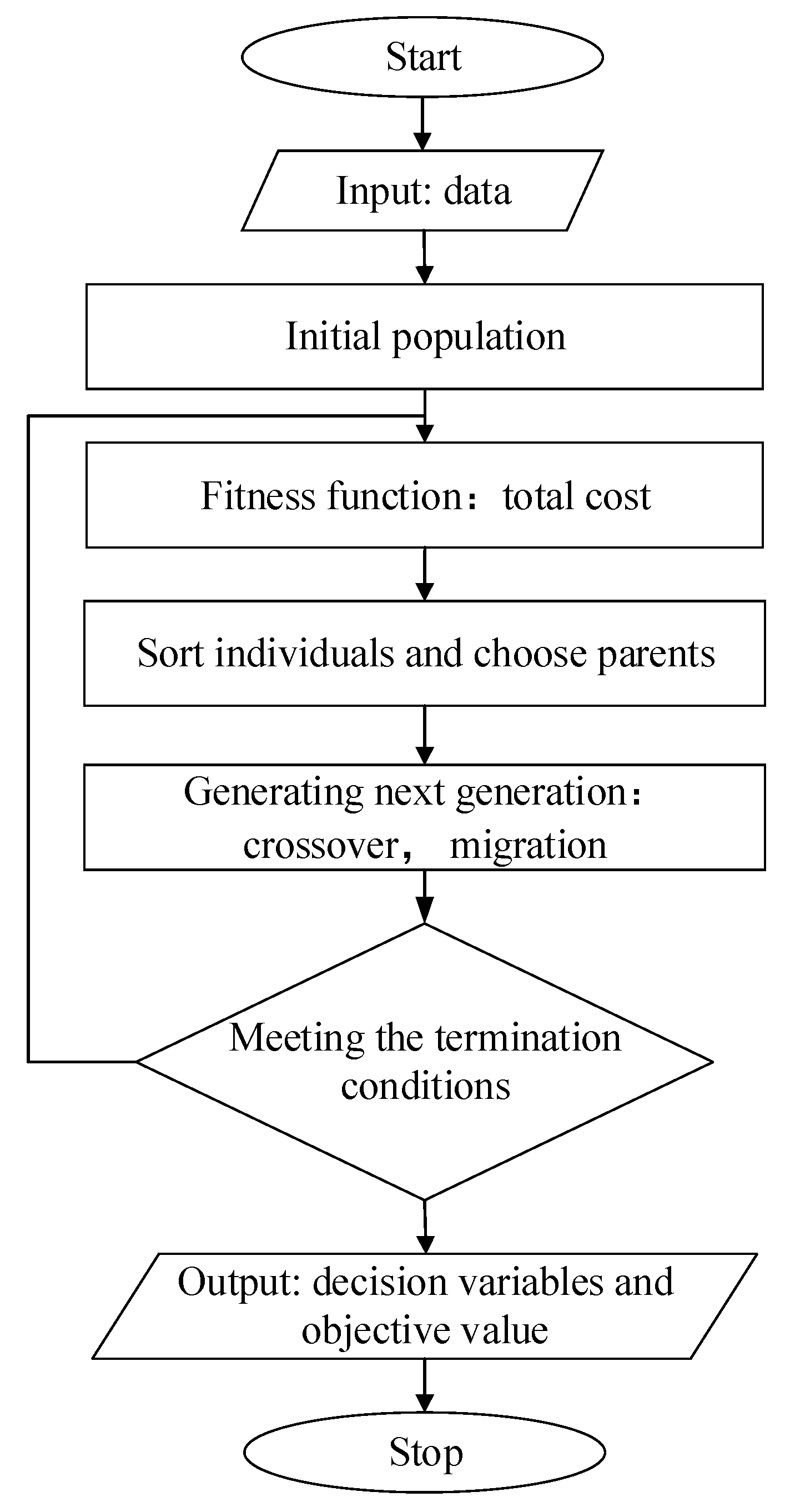
Genetic algorithms (GAs) have been comprehensively applied in the stop design of limited-stop services, such as in the studies by Qin [25], Han [26], Ye [27], and Zhang [28]. The optimal solution obtained by the Lingo software is the global optimal solution. Therefore, this study developed heuristic methods based on the GA and the Lingo software program to solve this problem. The two methods were compared. The application procedures for the genetic algorithm are shown in Figure 3. The problem was modeled in the GA using “Matlab optimtool”. The decision variables were coded as the double vector. The fitness function was the objective function of the proposed model. In this study, the population size was 50, the crossover fraction was 0.8, and the migration fraction was 0.05 [25]. Crossover combined two parents. To ensure that the children met the constraints, child1 = parent1 + 0.5a (parent2-parent1). a was a random number between 0 and 1. Based on “Matlab optimtool”, migration was set as “constraint dependent” to ensure the new chromosomes met the constraints. When the number of iterations reached 150, the solver stopped [25]. The application procedures for the Lingo software included input programming, software solutions, and output results.

The results obtained from the Lingo software and the genetic algorithm are given in

Table 2. The results of the case study in Jinan obtained by the Lingo software.

Variable	Value	Variable	Value	Variable	Value	Variable	Value
x1	1	x10	0	x19	0	x28	0
x2	0	x11	1	x20	1	x29	1
x3	0	x12	0	x21	0	x30	0
x4	1	x13	0	x22	0	x31	0
x5	1	x14	1	x23	1	x32	1
x6	0	x15	0	x24	0	x33	0
x7	1	x16	0	x25	0	x34	1
x8	1	x17	1	x26	1	HL (min)	8.5
x9	0	x18	0	x27	0	He (min)	15
C (h)	4352.80	CA (h)	419.86	CU (h)	3932.94

and

Table 3. The results of the case study in Jinan obtained by the genetic algorithm.

Variable	Value	Variable	Value	Variable	Value	Variable	Value
x1	1	x10	1	x19	1	x28	1
x2	0	x11	1	x20	0	x29	0
x3	1	x12	1	x21	0	x30	0
x4	0	x13	0	x22	1	x31	1
x5	0	x14	0	x23	0	x32	1
x6	1	x15	1	x24	0	x33	0
x7	1	x16	0	x25	1	x34	1
x8	0	x17	1	x26	1	HL (min)	8.5
x9	1	x18	0	x27	0	He (min)	16.5
C (h)	4367.94	CA (h)	310.95	CU (h)	4056.99

. In Table 2 and Table 3, if stop i is serviced by a limited-stop bus, x_i = 1, else x_i = 0; H_L and H_e respectively mean the headways of the local service and the limited-stop service during peak hours; C, C_A and C_U respectively mean the total cost, the agency cost, and the passenger cost of the bus service. The objective function of the Lingo software was less, although the difference in the total cost did not exceed 0.34%; the user cost in the Lingo software fell by 3%, and the agency cost increased by 25%. For the decision variables, the number of limited-stop serviced stops for the Lingo software and the genetic algorithm was 14 and 18, respectively; the headways of the local services were the same for the two methods, while the headways of the limited-stop service in the Lingo software decreased by 10%. It took 17 h to obtain the optimal solution model using the Lingo software, and the genetic algorithm’s solving time was less than 1 s.

For the proposed model, the Lingo software was better, and the reasons are as follows: (1) Lingo includes several ways to determine globally optimal solutions to nonlinear models; thus, Lingo can solve the proposed model, and the total cost and passenger cost will be obviously lower. Analyses of the influence of the increase in the limited-stop service fare and the bus corridor’s distance on the model’s results are described in the next section. The optimal solution can avoid interference from the local optimal solution. (2) Although the solving time of the genetic algorithm was less, the longer solution time by Lingo had no effect on the application of the model. The decision variables in this paper were the stops serviced as part of the limited-stop service and the headways of the limited-stop service and local service. The solutions for a model were relatively stable during the planning time; therefore, the solving time of the Lingo software can be accepted.

The results obtained by the Lingo software were compared with the local-only service. The comparison of the mixed service with the local-only service is presented in

Table 4. The comparison results.

Parameter	Mixed Service	Local-Only Service
C (h)	4367.94	4637.32
PL (p/h)	2398	2858
Pee (p/h)	210	-
PeL (p/h)	250	-
HL (min)	8.5	8
He (min)	16.5	-
CU (h)	4056.99	4427.89
CA (h)	310.95	209.43
VL (veh·km/h)	293.85	334.6
ML (veh)	26	35
WL (h)	0.069	0.058
TL (h)	0.82	0.86
vcL (km/h)	11.20	9.56
Ve (veh·km/h)	147.89	-
Me (veh)	8	-
Wee (h)	0.14	-
Tee (h)	0.44	-
WeL (h)	0.14	-
TeL (h)	0.41	-
vce (km/h)	18.39	-

. The stops for the limited-stop service were in locations with high demand, such as colleges, tourist attractions, high-tech zones, large residential communities, and transportation hubs, while the local vehicles serviced every stop, operating the same as prior to the implementation of the mixed service.

According to the results, the mixed service performed better than the local-only service. The total cost for the mixed model was 8% lower than that of the local-only service. The agency cost for the local-only service was lower because of the shorter travel distance per hour by vehicle. Travel speed had a great impact on the travel distance per hour for passengers. The average travel speed in the mixed service was much faster than that for the local-only service. In the mixed service, the travel speeds of limited-stop and local increased by 92% and 17%, respectively. The increased speed led to a significant decrease in passenger travel time, especially for the in-vehicle time. The average in-vehicle times for the limited-stop passengers and local passengers were reduced by −5% and −49%, respectively. For passengers, the average “door-to-door” travel time dropped by about 13%. Although the limited-stop service operated with a stop-skipping mechanism, about 76% of passengers were still served by the limited-stop service. The limited-stop service covered most of the passenger travel needs.

This case study demonstrates the applicability and reasonableness of the limited-stop and local mixed-service model. Compared with the local-only service, the level of service and the travel speed of the mixed service significantly increased. Thus, the mixed service improved the operational efficiency of the bus system for the bus agency, and the travel time of passengers dropped significantly. The mixed service not only met the commuters’ needs for fast travel along the corridor during peak hours but also maintained the accessibility of the bus stops. Based on the characteristics of Lingo software that can obtain the global optimal solution and facilitate the application of model results to practice, the proposed model was more suitable for solving through Lingo software.

4. Discussion

Under the given parameters, the design of the mixed-service model was proposed and solved. When the parameters change, the effects of the mixed service and local-only service need to be demonstrated. The ratios of the fare for the limited-stop service to the fare for the local service and to the bus corridor’s distance are critical for bus agencies and passengers. Therefore, it is necessary to evaluate the performance and competitiveness of the two types of services in different situations. Changes to the decision variables and the objective function under different hyper-parametrizations are also discussed.

4.1. Increase in the Fare

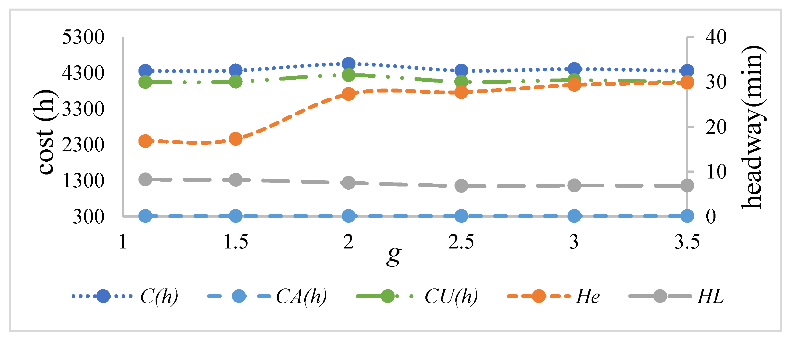
An increase in bus fares has impacts on both bus agencies and passengers. According to the transit willingness survey in Jinan, most passengers accepted that the ratio of the fare for the limited-stop service to the fare for local service, g, should be no more than 3.5. If g is greater than 3.5, passengers will choose other ways to travel. To explore the impact of the increasing fare on the bus agency and passengers, we tested the results of changing g from 1 to 3.5. The other parameters were the same. The total cost, agency cost, and passenger cost were not sensitive to the changes to g, as shown in Figure 4. The redistribution of vehicles and passengers in the limited-stop service and the local service restricted the change in costs. The increase in the fare had no significant impact on costs. When g < 1.5, the headways of the limited-stop service and the local service were stable. When g > 1.5, the headway of the limited-stop service increased significantly. The increased headway will cause an increase in the waiting time. The travel time approximately increased by 8 min, accounting for 15% of the total travel time of passengers. In addition, the passengers’ perceptual time increased by 42%. For passengers, the shorter in-vehicle time was offset by the longer waiting time of the limited-stop service, and the waiting time, especially, causes anxiety and discomfort for passengers. The total travel times for the two services were similar, and passengers chose the local service because of the higher fare for the limited-stop service.

Above all, if g is less than 1, the model has no feasible solution, and the losses for limited-stop service agencies will expand due to the operation of limited-stop services. However, if g exceeds 1.5, the number of limited-stop passengers will drop significantly. The advantages of the mixed service are very unnoticeable, and the competitiveness of the mixed service will decrease. Therefore, in order to ensure the enthusiasm of bus agencies to operate limited-stop services, as well as the performance of the mixed service, the ratio of the fare for the limited-stop service to the fare for the local service should be within the proper range.

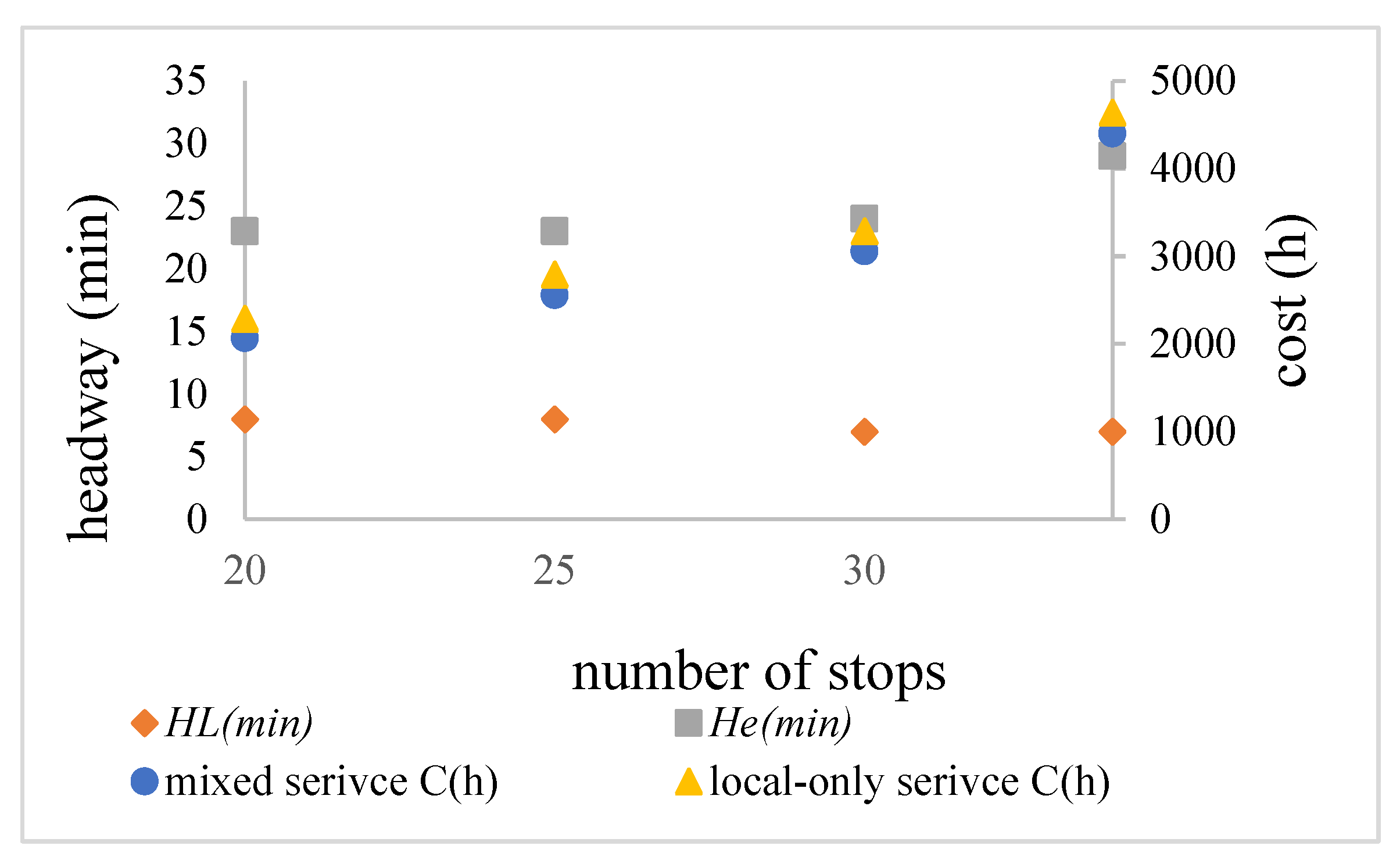
4.2. Bus Corridor’s Distance

Because a bus corridor’s distance is affected by the number of stops ($s_n$) and the average stop spacing ($\overline{s}$), the impacts of the two parameters were studied. When $s_n$ was analyzed, the values in the matrices P and D of the non-exited stops were also removed. The other parameters remained the same. When $\overline{s}$ was analyzed, the other parameters remained the same.

In Figure 5, with the increase in $s_n$, the costs of the two types of services increased. The mixed service performed better than the local-only service with the different values of $s_n$ owing to the stop-skipping mechanism of the limited-stop service. For the bus agency, when the number of stops changed, the design of the mixed service was not affected. H_e varied greatly, whereas H_L was relatively stable. The average waiting time for the limited stop service increased by approximately 5 min. The bus agency should add limited-stop vehicles to shorten the waiting time and maintain its competitiveness.

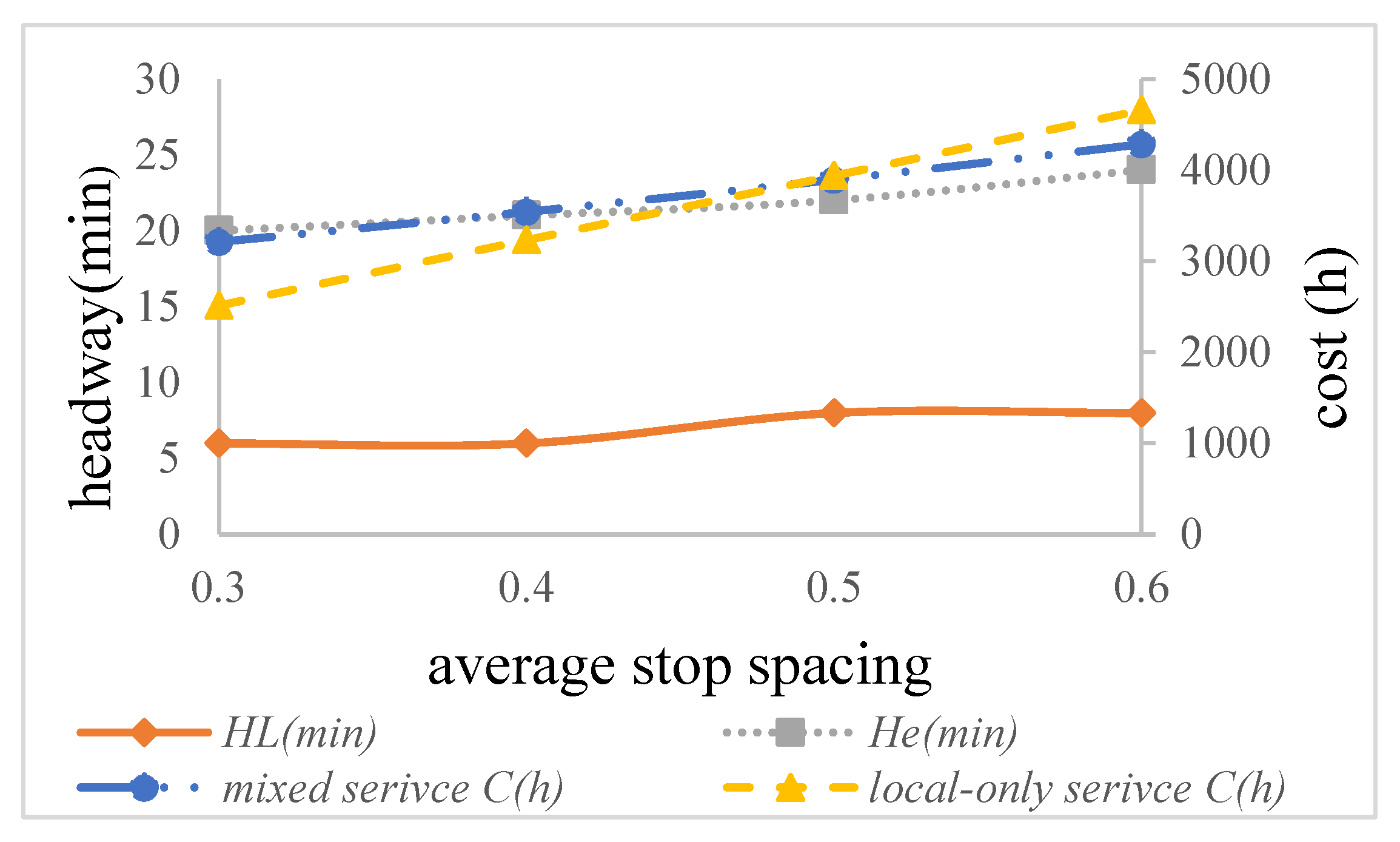
In Figure 6, when $\overline{s}$ < 0.5 km, the local service performed better than the mixed service. When $\overline{s}$ > 0.5 km and L > 16.5 km, the total cost of the mixed service was lower than that of the local service. With a longer average stop spacing, the advantage is that the decline in the in-vehicle time of the limited-stop service was more evident. The average stop spacing had a great impact on the efficiency of the mixed service and the local service. When the length of the bus corridor was longer than 16.5 km and the average bus stop spacing was longer than 0.5 km, the mixed service design was more conducive to improving the performance of the bus. When $\overline{s}$ changed from 0.3 to 0.6 km, the average waiting time increased by approximately 2 min, which is within acceptable bounds for passengers. The change in waiting time had no notable impact on the service level of the limited-stop service.

Above all, when stops are added or removed from the bus route, the mixed service will still be better than local services for new routes. The average stop spacing had a large impact on the bus service. As the distance of the corridor and the average stop spacing increased, the mixed service was more prominent, and the design of the mixed service was more gainful and suitable.

4.3. Different Hyper-Parametrizations

The rates of change for the decision variables and the coefficient of elasticity of the objective function when a unit change in the hyper-parametrizations occurred are shown in

Table 5. The rates of the headway changes.

	v	$\mathit{\tau }$	$\mathit{\tau }\prime$	M	wA	ww	vw	$\mathit{\mu }$	$V	$M
HL	−24%	−3%	−3%	−24%	−3%	0%	−21%	−3%	−7%	−7%
He	14%	0%	0%	0%	0%	0%	14%	0%	0%	0%

and

Table 6. The objective function elasticity coefficient.

	v	$\mathit{\tau }$	$\mathit{\tau }\prime$	M	wA	ww	vw	$\mathit{\mu }$	$V	$M
EIC	−0.4	0.1	0	−0.1	0.3	0.2	−0.4	0	0	0
EICA	−1	−0.1	−0.2	1	0.2	−0.5	−0.3	−0.6	−0.3	−0.6
EICU	0.1	0.2	0.1	−0.9	0.5	0.3	−1	0.5	0	0.4

, respectively.

Stops for the limited-stop service were primarily affected by the OD matrix; therefore, when a unit change in the hyper-parametrizations occurs, stops for the limited-stop service remain unchanged. Adding vehicles and increasing the travel speed decreased the headway of the local service by 24%. The effects of the other hyper-parametrizations were smaller for the headways. The variation in the headway of the local service was between −17.5% and 15%, and the variation in the headway of the limited-stop service was between −4% and 12%. Overall, the model’s stability was good.

The elasticity coefficient of the total cost was small, and the model was robust. The passenger cost showed inelastic results for most of the parameters. The elasticity coefficient of the passengers’ speed when entering or leaving the bus system to the passenger cost was −1; thus, the passenger cost significantly decreased when passengers entered or left the bus system using faster methods such as by bike-sharing, “P + R”, and “K + R”. The elasticity coefficients of the bus cruising speed and the number of vehicles to the agency cost were −1 and 1, respectively. Therefore, increasing the cruising speed, such as by implementing bus lanes, can help to significantly reduce the agency cost. Adding to the number of vehicles significantly raised the agency cost. The other input parameters produced a small effect on the costs.

5. Conclusions

Limited-stop services reduce passenger travel time and increase bus operating speed. However, they can also lead to adverse outcomes such as a decline in limited-stop service ridership and a decrease in bus fare revenue. At present, there are few studies that have focused on the impact of an increase in a limited-stop service’s fare. This study proposed the design of a limited-stop and local mixed bus service model, which determined the stops of the limited-stop service and the headways of the limited-stop and local services. A limited-stop fare increase was carried out in the model so that the agencies will not expand losses due to operating a limited-stop service. In this model, the goal was to minimize total cost, including passenger cost and agency cost. The advantages of limited-stop service cannot be reflected in short bus lines. In order to determine the conditions applicable to mixed service, this study evaluated mixed service performance under different distances of the bus corridor. The impacts of the key hyper-parametrizations to the costs and headways were also discussed. The solutions obtained by the Lingo software and the GA were compared to choose a better algorithm for the proposed model. Although the solving time of Lingo was longer, the long solution time had no effect on the application of the model. The global optimal solution obtained by the Lingo software was more beneficial, and Lingo software was better for the proposed model.

Based on the results confirmed by the model output from the case study in Jinan, China, an evaluation of the mixed service in Jinan for No. 115 was conducted. It was shown that ignoring increased fare for limited-stop service and applicable conditions of mixed service will reduce the effectiveness of limited-stop service and lead to potential planning errors. We found that an appropriate range of fares for limited-stop service enhanced the bus company’s motivation to operate limited-stop service, as well as the competitiveness of limited-stop service. It was also shown that mixed-service operations can achieve a win–win situation for bus agents and passengers. To achieve this goal, the mixed service should operate within a profitable service zone and with a considerable bus corridor distance. With an increase in the corridor distance, the local-only service’s competitiveness decreased, and the performance of the mixed service was highlighted. The average stop spacing had a large impact on the bus service. The results of this study are useful for bus agencies to determine the applicable conditions for mixed services and the range of increased fares for limited stops when designing a limited-stop service.

In future research, it will be necessary to extend the proposed model to the whole transit network with transfers. Furthermore, other factors, such as uneven stop spacing and the impacts of electric vehicles [29], will be added to the model, making the results more realistic.