Article

Statistical Characterization of Boundary Kinematics Observed on a Series of Triaxial Sand Specimens

by
Yichuan Zhu
1,* and
Zenon Medina-Cetina
2,*
1
Civil & Environmental Engineering Department, Temple University, Philadelphia, PA 19122, USA
2
Zachry Department of Civil & Environmental Engineering, Texas A&M University, College Station, TX 77843, USA
*
Authors to whom correspondence should be addressed.
Appl. Sci. 2022, 12(22), 11413; https://doi.org/10.3390/app122211413
Submission received: 17 October 2022 / Revised: 1 November 2022 / Accepted: 5 November 2022 / Published: 10 November 2022

Abstract

:
This paper follows up on a reference paper that inspired MDPI’s topic “Stochastic Geomechanics: From Experimentation to Forward Modeling”, in which the authors populated a spatio–temporal database of boundary displacement fields from a series of triaxial sand specimens using three-dimensional (3D) digital image correlation analysis. The database was curated and is currently available to the scientific community for further study. This paper uses a subset of this database, in which the experimental conditions were similar, to statistically investigate the dominant kinematic phenomena observed on the boundary of triaxial sand specimens under compression. The first-order 3D kinematic operators under the cylindrical coordinates, comprised of the divergence, curl, and gradient, were applied to the boundary displacement fields to illustrate the localization deformation patterns including the translational, rotational, shearing, and volumetric behaviors throughout the triaxial compression processes. Subsequently, the first-order statistics of the kinematic results are estimated, with the aim of revealing the evolution of associated localization effects as well as their corresponding uncertainties in space and time. The results of this research provide an innovative statistical interpretation of the localization effects on soil specimens under three-dimensional stress conditions. The proposed approach advances the interpretation of granular material’s responses under triaxial compression experimental conditions, while opening an opportunity to reproduce the material’s kinematic responses under the triaxial experimental conditions through constitutive modeling or machine learning techniques.

1. Introduction

This research ensued from three reference papers: the first introduced the experimental methods and sample characteristics of an experimental database describing both global and local deformation effects on triaxial sand specimens [1]; the second further conducted the spatio–temporal statistical analysis based on the populated database [2]; in the third paper [3], a set of first-order kinematic operators in cylindrical coordinates were introduced and applied on a set of experiments under varying experimental conditions to study the variability of localization effects in triaxial sand specimens. Based on these preceding contributions, this paper used a subset of the aforementioned experimental database, in which the experimental conditions were similarly controlled, to investigate the dominant mode and variability of strain localizations in triaxial sand specimens.
The definition of strain localization here refers to non-homogeneous deformation that occurred in a material when subjected to compressive or tensile stresses. The accumulation of strain localization is commonly seen within a thin zone of intense deformation, such as dilation, contraction, and/or rotation leading to the formation of shear bands, which encompass the major material responses once these are fully formed [4]. To better understand the effects of strain localization, it requires a sensing method that can capture the non-homogeneous deforming features in a deforming body, in contrast to conventional global-scale measurements such as axial stress versus strain and volumetric strain versus axial strain descriptions that can produce, at best, the volume-averaged deformational characteristics. That is, it is assumed that the specimen has a homogeneous structure.
Within the geotechnical engineering community, the development of X-ray tomography and digital image correlation (DIC) methods have provided effective means to advance the elucidation of strain localizations in granular materials and sands, in particular. For instance, Roscoe [5] used a 150 kV X-ray apparatus to check the large dilatancy within the shear band in a retaining wall model. Starting from the 1980s, Desrues et al. [6,7,8] used X-ray tomography to study various localization effects in sands, including the thickness, orientation, and volumetric dilation of the shear band. The more recent advent of the microfocus X-ray tomography system has enhanced the resolution of specimen imaging, which allows for microstructure and particulate behavior to be illustrated during the shearing of geo-material. For instance, Oda et al. [9] used microfocus X-ray tomography to examine column-like structures in a shear band. Alshibli et al. [10,11] used 3D synchrotron microcomputed tomography to investigate particle translation and rotation, as well as the microband development that precedes the occurrence of persistent shear bands.
Apart from X-ray tomography methods, DIC represents another emerging sensing technique that can sample high-resolution displacement fields along the exterior surface of the testing specimens. Compared to X-ray tomography, internal sampling is usually not allowed for DIC methods. Nevertheless, the high-frequency imaging process permits the almost continuous spatio–temporal description of the deforming surface that is critical in the study of localization effects considering that the onset or evolution of strain localization and bifurcation can take place over a very short time window [8], which could be smeared out if the sampling step is large. The DIC methods used in strain localization research have also offered insights on the triggering of the persistent shear band formation, vortex structures, and the build-up and collapse of force chains, among others that can be found in [12,13,14,15,16,17].
Despite these studies considering the discrete nature of sands when investigating the localization effects, the spatial derivative of the displacement field, which associates to the relative movements of soil particles and the calculation of strain tensors, has not been directly characterized. To address this challenge, the seminal work of Zhang and Regueiro [18] proposed seven finite strain measures that can derive the deformation gradient  F ¯ n + 1 based on the 3D discrete element method (DEM) simulations. Building on this concept, Amirrahmat et al. [19] calculated the Eulerian strain tensor based on the experimental data of 3D X-ray-computed tomography. The methodology provided in such analyses bridged the findings of strain localization at the micro- and meso-scales, which are complementary to each other, thus both particulate and relative deformations at the local areas were identified.
In a more recent work, Zhu and Medina-Cetina [3] proposed the illustration of the kinematic phenomena in the cylindrical coordinate system, in which the orthogonal axes coincide with the principal stress directions of the triaxial compression setting on a cylindrical specimen. Their findings provided a new research perspective by presenting the interactions between different localization effects consisting of dilation, contraction, and rotation, during the specimen’s failure process.
In this paper, the authors used the same kinematic operators proposed by Zhu and Medina-Cetina [3], but with the objective of providing an innovative characterization of the dominant mode and the uncertainty of strain localizations in sand, due to the availability of an experimental database where tests were conducted under similar experimental conditions. Therefore, the research focus is driven by the inherent acknowledgement of randomness associated with the localized material behavior, which naturally leads to a variable failure mechanism, in contrast to homogeneous geomaterial assumptions made for most global constitutive studies.
After selecting a set of 3D-DIC measurements of triaxial sand specimens, and after populating each test’s localization properties as kinematic fields (spatio–temporal), the mean and standard deviation fields were computed over four selected kinematic properties, to reveal the evolution of associated localization effects as well as their uncertainties in space and time. The novel statistical insights of strain localization offered in this work can serve as the basis for reproducing the soil’s responses through kinematics-based constitutive modeling or machine learning methods, which can further impact the study of uncertainty quantification on the soils’ mechanical behaviors. All supporting data and models needed to reproduce this paper are available at https://dataverse.tdl.org/dataverse/SGL, accessed on 1 October 2022.

2. Experimental Method

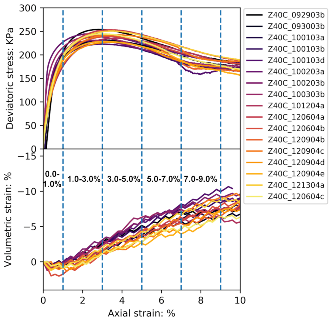
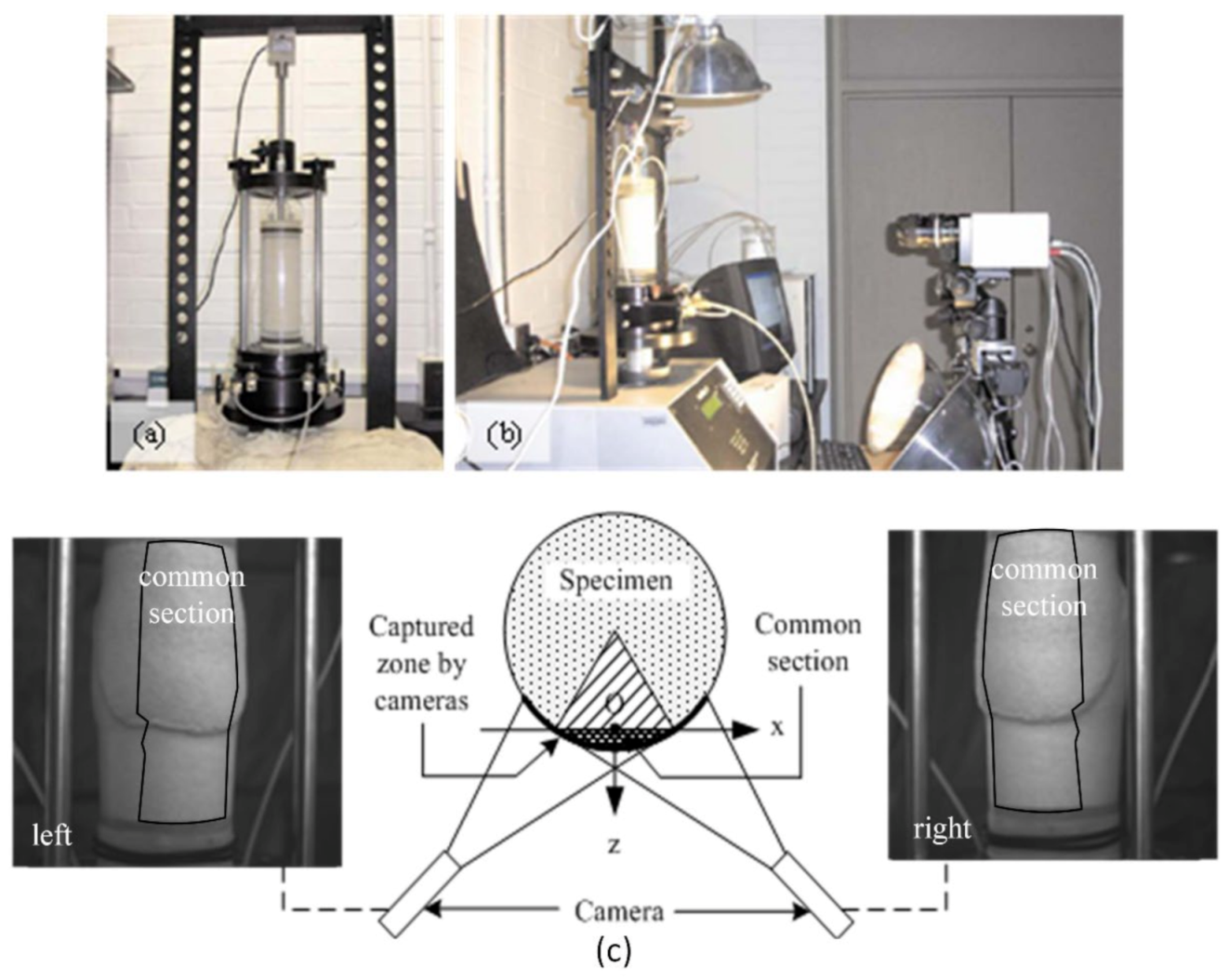
2.1. Triaxial Compression Test

Dry sand, classified as SP, was used to constitute the testing specimens for triaxial compression tests. The median particle size was 0.50 mm, and the coefficients of uniformity and curvature were 2.34 and 1.11, respectively. In this research, a subset of the database as populated in Medina-Cetina et al. [1] was used, in which the experimental conditions were nominally similar, to study the dominant mode and uncertainty of localization effects in sand. Table 1 presents the specimen characteristics of 17 participating tests and the basic statistics of each specimen parameter. Thirteen testing specimens were vibratory compacted in three layers, and four specimens were prepared through dry pluviation with a carefully controlled drop height to reach a similar initial density. In the bottom row of Table 1, the standard deviation quantities show that the magnitude of variation of the specimen parameters is relatively small, suggesting that all the specimens were nominally similar in the global sense and thus suitable for representing the data population under the current experimental conditions.
The experimental process was practically similar to a conventional triaxial test. However, the Plexiglas cell used for confinement was removed, and the specimen was consolidated at a 40 kPa confining pressure through the use of a vacuum pump. The axial loading was applied to the specimen with a strain-controlled manner ( ε ˙ = 0.2 % / min ) along the direction from the bottom up. Two digital cameras were placed in front of the testing sample, namely Q-Imaging PMI-4201, capturing synchronous images of the deforming specimen at every 0.05% of axial strain. Figure 1 shows the stress–strain and volumetric–axial strain responses of all 17 tests, from 0.0 to 9.8% of axial strain. The volumetric strains in this study were estimated through the reconstruction of specimen geometry by taking advantage of the DIC-sampled boundary evolution. Specifically, we assume the specimen’s volume is a sum of a series of “stacked disks”. The height of each disk was determined as 1 mm, and the diameter was calculated from the average radius derived from the DIC analysis at the corresponding height of the specimen. Equation 1 shows the method to integrate all volumetric disks to estimate the bulk volume of the specimen. The precision and accuracy of this indirect approach to measure the specimen’s volumetric strain are thus dependent on the quality and characteristics of the sampled DIC datasets. The calibrations show that this technique was in good agreement with the conventional volumetric strain measurement as demonstrated by several previous studies [1,20,21]:
V = 0 H 0 2 π 0 R r   dr   d θ   dz = 0 H 0 2 π 1 2 R 2   d θ   dz = 1 2 R 2 2 π 0 H dz = π 0 H R 2 dz
The dashed intervals indicate the strain windows for the kinematic analysis that is detailed in the proceeding sections. The axial stress–strain curves anticipate the development of strain bifurcation effects among all tests in the pre-peak regime, while the variability remains stable after the peak stress. The volumetric strain presents first a compression and then a dilation pattern, which is anticipated for the dense specimens. Different from the post-peak homoscedastic behavior presented by the stress–strain curves, the scattering is continuous for volumetric–axial strain responses throughout the tests. For a systematic evaluation of the spatio–temporal statistical characteristics of the data ensemble under the multi-dimensional conditions, readers are referred to a previous publication that is included in the same MDPI’s Topic “Stochastic Geomechanics: From Experimentation to Forward Modeling” [2].

2.2. 3D-Digital Image Correlation (3D-DIC)

The 3D-DIC is a non-intrusive experimental method to sense the displacement field on a deforming surface. The basic unit of DIC analysis is a subgroup of image pixels, called a subset, which is comprised by a cluster of sand colors manifested through the latex specimen membrane. Due to sand grains being naturally characterized with color variations, each subset is in stereo images possessing a unique mathematical entity that can be identified through pattern recognition. In the present research, two digital cameras were set up in front of the specimen with different orientation angles while focusing on the common area of the specimen surface. The 3D specimen boundary can be reconstructed through synchronous images captured by these two cameras, based on the principle which is similar to the way that human eyes perceive position and shape of an object. Displacement is derived by mapping the overlapping subsets between two digital images, and consequently the deforming vectors are defined by translational, rotational, and shearing quantities of subsets in 3D space. Cubic spline interpolation was used to track the trajectory of subsets over several incremental images referenced to the initial material coordinates. The displacement measurements covered a sector about 85 degrees around the specimen circumference, and yielded approximately 40,000 displacement vectors in each sampling with a resolution of 0.4 mm from center-to-center of the subsets. The 3D-DIC-coupled triaxial compression system is described in Figure 2.
Figure 3 plots a typical 3D-DIC result of the displacement field for test 092903b between a global axial strain of 3.0% and 9.0%. The contours that indicate displacement quantities (in millimeters) along each axis are superimposed on the deformed body of axial strain at 9.0% (Eulerian description). The first row of Figure 3 shows displacements along horizontal (u), vertical (v), and out-of-plane (w) directions from left to right, respectively. The horizontal displacement field (u field) indicates the specimen was expanded in the middle and that can be associated with the development of the expansion band. The vertical displacement field shows that significant motion was concentrated at the bottom of the specimen, which is caused by the bottom-up loading method. The out-of-plane displacement field (w field) explicitly depicts the areas of expansion, in contrast to the top and bottom of the specimen, which presents approximately zero out-of-plane displacements. The second row of Figure 3 is the same displacement field, but decomposed in the cylindrical coordinate system, showing displacement fields along the radial (r), tangential (t), and axial (v) directions. Notice that the radial displacement (r) correlates with the developed expanding region at the present stage of loading. A shear banding area, suggested by intense clockwise rotation in the tangential displacement field (t field), is observed along the diagonal direction of the specimen’s surface. The vertical displacement field (v) is the same vector component v as defined in Cartesian coordinates.

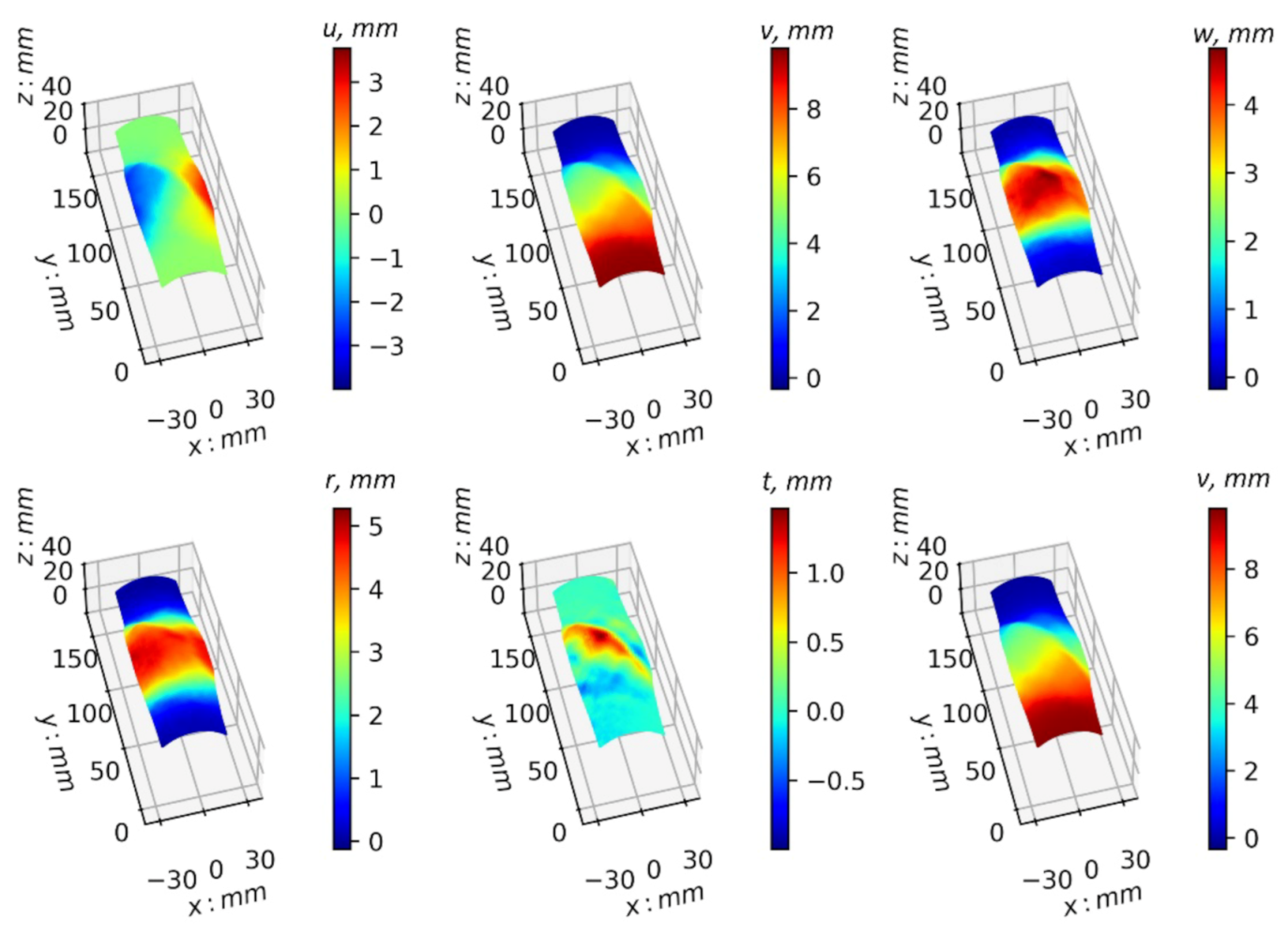
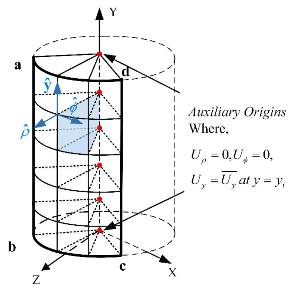
3. 3D Kinematics of the Boundary Displacement Field

To characterize the 3D kinematic properties of displacement fields, it is a prerequisite to define the 3D basic unit, which kinematic operators can apply. Figure 4 gives a schematic illustration of a 3D basic unit that is defined for the present kinematic analysis. In this study, a series of auxiliary origins along the axial direction of the specimen are assumed, for which the radial and tangential displacements are assumed to be zero; the axial displacements are evaluated as the averaged vertical displacements sampled along the boundary at each specimen height. This assumption is inspired and supported by the experimental observations of Desrues et al. [7]: according to the X-ray tomography results that the deformed sand specimen consists of a rigid cone located along the axis of the specimen, and several shear planes extending outwards from the cone to the specimen boundary, which implies that the radial and tangential displacements along the axis are negligible compared to the displacements along the vertical direction. The defined auxiliary origins are then linked with the boundary coordinates used in the DIC analysis, to form the basic unit for kinematic analysis in cylindrical coordinates.
In a preceding paper by Zhu and Medina-Cetina [3], the authors have provided the first-order kinematic operators in cylindrical coordinates. Specifically, the first-order kinematics comprised of gradient, divergence, and curl fields that are produced by applying the nabla operator to the vector field U [22]. The gradient is a tensor product between the nabla operator and the 3D vector field U (Equation (2)), which includes nine derivative components representing translational or rotational deformations of a local area. The sum of three diagonal terms is the divergence of the vector field U (Equation (3)), which indicates the volumetric sink (negative quantities) or source (positive quantities) of a local area. The curl contains three terms c u r l U ρ , c u r l U ϕ , and c u r l U y representing local rotational deformations along the ρ ^ , ϕ ^ , and y ^ axes, respectively (Equation (4)):
g r a d U = U = F 11 F 12 F 13 F 21 F 22 F 23 F 31 F 32 F 33 = U ρ ρ 1 ρ U ρ ϕ U ϕ U ρ y U ϕ ρ 1 ρ U ϕ ϕ + U ρ U ϕ y U y ρ 1 ρ U y ϕ U y y
d i v U = U = 1 ρ ρ U ρ ρ + 1 ρ U ϕ ϕ + U y y
c u r l U = × U = c u r l U ρ + c u r l U ϕ + c u r l U y = ρ ^ 1 ρ U y ϕ U ϕ y + ϕ ^ U ρ y U y ρ + y ^ 1 ρ ρ U ϕ ρ 1 ρ U ρ ϕ
Figure 5 provides an example of a divergence field of test 092903b at axial strains between ε a = 0.0 % and ε a = 9.0 % . Subplots in Figure 5a,b show the specimen image and stress–strain response at an axial strain of ε a = 9.0 % . Figure 5c plots the corresponding divergence field that shows the local volumetric dilation (+) and contraction (−). The results show that volumetric dilation occurs in the middle of specimen, which corresponds to the development of an expansion band. Above and below the expansion band, two compaction bands developed, and were distributed horizontally. The shear band presented in the specimen’s image (Figure 5a) is explicitly identified by the divergence field, manifested as a localized intense dilation or as contraction zones, depending on its intersection with the expansion or compaction band.
It is important to note that the above definitions of gradient, divergence, and curl can be also used to deduce other strain measures, such as rotational strain, Lagrangian strain, Green or Almansi strain tensors, and others, in a cylindrical coordinate system. This mathematical refinement can potentially reveal new localization evidence with sand materials. Moreover, the methodology is not only suitable for boundary kinematic analysis, but also applicable to the X-ray tomography-sampled displacement field, which possesses a further capacity to describe internal deformations. Outcomes from these studies are expected to offer new insights of localization effects that can complement current findings on the localization effects of materials in general.

4. Statistical Characterization of Boundary Kinematics on Triaxial Sand Specimens

4.1. Experimental Design

The authors formulated an experimental design to specify the method for conducting a statistical analysis toward boundary kinematics. This consists of five strain levels, comprised of 0.0% to 1.0%, 1.0% to 3.0%, 3.0% to 5.0%, 5.0% to 7.0%, and 7.0% to 9.0%, selected as incremental steps as shown in Figure 1. The first two axial strain levels are associated with the elastic and hardening phases of the material’s response. The peak stress was reached at approximately 3.0% of axial strain for most of the tests, subsequently the stress-strain responses showed softening until 9.0% of axial strain that presented with the onset of the critical state.
Figure 6 presents the experimental design of the statistical characterization. Four kinematic properties, including the gradient along the ρ ^ axis ( F 11 ), gradient along the y ^ axis ( F 33 ), divergence ( d i v U ), and curl along the ρ ^ axis ( ( c u r l U ) ρ ), were calculated on all the 3D-DIC-sampled displacement fields, and the results were used for subsequent statistical characterization. These chosen kinematic properties are tightly associated with different localization effects of the triaxial sand specimen. For instance, F 11 indicates the radial deformation gradient that can reflect the development of the expansion band, F 33 indicates the vertical deformation gradient that can relate to the vertical compression inside the shear band, d i v U presents the volumetric change of the specimen, and ( c u r l U ) ρ indicates the rotational deformation pertaining to the widely reported phenomenon of intense inter-particle rotations inside the shear band [8,9,15,17]. The calculated mean and standard deviation fields were plotted overlaying the averaged boundary shape of specimens, to overcome the challenge that each specimen has its own distinctive boundary shape. The Lagrangian description of a displacement field was adopted, meaning that the kinematic quantities were computed from the reference to the initial image of each strain window.

4.2. Statistical Characterization of the Evolution of the F 11 Field

The gradient along the ρ ^ axis ( F 11 ) as mentioned in the preceding sections indicates the radial deformational behavior of a specimen, which can signify the development of a radially expanding or compressing region. The statistical analyses performed here include the mean and standard deviation of the F 11 fields in space and time (Figure 7 and Figure 8), which associates with the dominant mode and uncertainty evolutions of expansional banding phenomena. All results in this and the following sections are plotted on both the varying and consistent magnitude scales as shown in Figure 7 and Figure 8, for clear presentation of small quantities in particular, at initial stages, meanwhile allowing for comparative analyses that require a consistent value range. The mean field of F 11 indicates that a growing rate of budging has occurred in the specimen from the start to the early softening stage ( ε a = 5.0 % ). However, this trend gradually declined, particularly when the test approached the critical state ( ε a = 9.0 % ). A possible explanation is that other localization effects, such as the shear band and/or compaction band, have dominated the later stage of deformation and relaxed the energy accumulated on the earlier developed expansion band. It is also worth noting that the horizontally uniform distributed expansion region morphed into an irregular shape after an axial strain of ε a = 5.0 % , which is again hypothesized due to the build and interaction between a radially expanding region and other banding phenomena. Figure 8 shows the evolution of the standard deviation fields of F 11 . After the peak stress ( ε a = 3.0 % ), a crater-like uncertainty pattern emerged to the center of the specimen, with low uncertainty in the middle, while high uncertainty zones were distributed along the surrounding areas. This observation indicates that most of the specimens expanded with a similar trend in the middle part, but presented with varying patterns along other boundary areas.

4.3. Statistical Characterization of the Evolution of the F 33 Field

The gradient along the y ^ axis F 33 specifies local deformations along the axial direction. Figure 9 shows an intense axial compression zone coinciding with a significant radial deformation region observed in the hardening phase ( ε a = 1.0 3.0 % ), subsequently the localization was initiated after the peak stress ( ε a = 3.0 % ). In the later softening stage, the intense axial compression is seen exclusively localized inside the shear bands, which are distributed along the diagonal and anti-diagonal directions along the specimen. The standard deviation plot (Figure 10) shows a similar localization pattern as higher uncertainty areas are concentrated inside the shear bands, suggesting that once the persistent shear band is fully formed, a local axial compression of major significance is only observed inside the shear bands.

4.4. Statistical Characterization of the Evolution of the d i v U Field

The divergence field d i v U indicates the local volumetric dilation or contraction behaviors. Figure 11 presents the evolution of the mean field of d i v U in space and time, which indicates a chronological order of expansion–compaction bands’ behavior. Since this represents the sum of all components on the principal directions, predominant rates of change may dominate the highest and lowest divergence estimates. The local dilation, which is mainly presented in the middle of specimen, was initiated immediately after the test started ( ε a = 0.0 1.0 % ). The bulging of the specimen led to the volumetric expansion gradually localized in the middle of the specimen where a uniform expansion region formed, which reached its peak value around the start of the softening stage ( ε a = 3.0 5.0 % ). In the next strain level ( ε a = 5.0 7.0 % ), the expanding behavior declined, and two compaction bands formed at the top and bottom of the specimen, illustrating a change of the dominant volumetric behavior. Figure 12 presents the evolution of the standard deviation field of d i v U . The uncertainty is seen localized during the late softening stage ( ε a = 5.0 7.0 % ), and is concentrated in the compaction band areas, which may be an indication of the varying intensity and/or location of occurrence of the compression bands. Overall, the statistical characterization of the d i v U field suggests a chronological order regarding the appearance of expansion and compaction bands, with the latter possessing more uncertainty as shown in its spatio–temporal descriptions.

4.5. Statistical Characterization of the Evolution of the ( c u r l U ) ρ Field

The curl field along the ρ ^ axis ( ( c u r l U ) ρ ) represents the rotational deformation gradient along the ρ ^ axis, which can be used to indicate the development of a shear band. The mean plots of the ( c u r l U ) ρ fields (Figure 13) suggest that the strain bifurcation initiated from the hardening stage ( ε a = 1.0 3.0 % ), which can be associated with the development of micro shear bands [11]. In total, three persistent shear bands were fully formed at the loading stage of ε a = 5.0 7.0 % . The inclination angle measures show that the shear band has a steeper orientation when it appears to the middle compared to the upper and lower parts of the specimen. The authors consider this is due to the development of compaction bands that decreased the vertical movement of the soil particles in their corresponding regions, which resulted in a more horizontal orientation in the upper and lower parts of the specimen. Figure 14 shows the standard deviation of the ( c u r l U ) ρ fields, in which the uncertainty is seen highlighted within the shear bands once they were fully established ( ε a = 5.0 7.0 % ), suggesting varying strain localizations may be due to different a rotation intensity and/or location when compared with other regions within the specimen.

5. Conclusions

Sand can be defined as a heterogeneous granular material with respect to its geo-chemical compositions and mechanical properties. This naturally leads to variable failure mechanisms, including localization effects, which for sands can be sensed over the boundary of testing cylindrical specimens when subjected to compressive or tensile stresses. This paper presented a study to characterize the dominant patterns and their corresponding uncertainty in terms of localization effects, when associated with laboratory triaxial sand specimens, by computing first-order statistics (i.e., mean and standard deviation) of a data ensemble comprised of local kinematic effects sensed via a 3D-DIC. The main findings of this research include:
(1)
The onsets of expansion and compaction bands follow a chronological order and dominate the main volumetric behavior of the specimen at different loading stages, with a watershed point around an axial strain of ε a = 5.0 % that corresponds to the early softening stage;
(2)
The inter-particle rotation and axial compression are two main kinematic phenomena that appeared from the persistent occurrence of shear band developments. The former is more evident when shear bands develop further within the specimen’s central expansion region, and the latter is as a result of interactions between the shear band and the compaction bands. These kinematic properties can be further related to the formation and buckling of force chains, which warrants a future study to investigate such phenomena according to sands’ particulate behaviors;
(3)
The orientation of a shear band can be influenced by the development of expansion and compaction bands. In addition, the local axial strain can be localized inside a persistent shear band once it is fully formed;
(4)
The uncertainty analyses show that more variability is associated with the development of compaction and shear bands, compared to that of expansion regions. Also, the intensity of the kinematic phenomena and the location of these may contribute to the increased randomness captured closer to the upper and lower boundaries of the specimen.
It is important to note that the statistical analysis presented in this study also forms the basis for reproducing the soil’s responses through new kinematics-based constitutive modeling or machine learning methods, which can further impact the study of uncertainty quantification on soil’s mechanical behavior. A series of follow up papers will capitalize on the improved modeling of sands thanks to the three papers published in series as part MDPI’s Stochastic Geomechanics topic.

Author Contributions

Conceptualization, Y.Z. and Z.M.-C.; data curation, Y.Z. and Z.M.-C.; funding acquisition, Z.M.-C.; investigation, Y.Z. and Z.M.-C.; methodology, Y.Z.; project administration, Y.Z. and Z.M.-C.; resources, Z.M.-C.; supervision, Z.M.-C.; validation, Y.Z. and Z.M.-C.; visualization, Y.Z.; writing—original draft, Y.Z.; writing—review and editing, Z.M.-C. All authors have read and agreed to the published version of the manuscript.

Funding

The research presented in this paper was sponsored by multiple agencies, including the National Science Foundation (NSF), Consejo Nacional de Ciencia y Tecnologia (CONACYT), and Texas A&M University (TAMU).

Institutional Review Board Statement

Not applicable.

Informed Consent Statement

Not applicable.

Data Availability Statement

The experimental data supporting the findings of this paper are provided along with the article and made available at the Texas Data Repository (https://dataverse.tdl.org/dataverse/SGL-MDPI-Topic-StochasticGeomechancis-ForwardModeling) (accessed on 1 September 2022). Additional queries may be directed to the corresponding author.

Conflicts of Interest

The authors declare no conflict interest.

References

  1. Medina-Cetina, Z.; Song, A.; Zhu, Y.; Pineda-Contreras, A.R.; Rechenmacher, A. Global and Local Deformation Effects of Dry Vacuum-Consolidated Triaxial Compression Tests on Sand Specimens: Making a Database Available for the Calibration and Development of Forward Models. Materials 2022, 15, 1528. [Google Scholar] [CrossRef] [PubMed]
  2. Zhu, Y.; Medina-Cetina, Z.; Pineda-Contreras, A.R. Spatio-Temporal Statistical Characterization of Boundary Kinematic Phenomena of Triaxial Sand Specimens. Materials 2022, 15, 2189. [Google Scholar] [CrossRef] [PubMed]
  3. Zhu, Y.; Medina-Cetina, Z. Assessment of Spatio-Temporal Kinematic Phenomena Observed along the Boundary of Triaxial Sand Specimens. Appl. Sci. 2022, 12, 8091. [Google Scholar] [CrossRef]
  4. Rechenmacher, A.L.; Finno, R.J. Digital Image Correlation to Evaluate Shear Banding in Dilative Sands. Geotech. Test. J. 2003, 27, 13–22. [Google Scholar] [CrossRef]
  5. Roscoe, K.H. The Influence of Strains in Soil Mechanics. GÉOtechnique 1970, 20, 129–170. [Google Scholar] [CrossRef]
  6. Desrues, J.; Lanier, J.; Stutz, P. Localization of the Deformation in Tests on Sand Sample. Eng. Fract. Mech. 1985, 21, 909–921. [Google Scholar] [CrossRef]
  7. Desrues, J.; Chambon, R.; Mokni, M.; Mazerolle, F. Void Ratio Evolution inside Shear Bands in Triaxial Sand Specimens Studied by Computed Tomography. GÉOtechnique 1996, 46, 529–546. [Google Scholar] [CrossRef]
  8. Desrues, J.; Viggiani, G. Strain Localization in Sand: An Overview of the Experimental Results Obtained in Grenoble Using Stereophotogrammetry. Int. J. Numer Anal. Methods Geomech. 2004, 28, 279–321. [Google Scholar] [CrossRef]
  9. Oda, M.; Takemura, T.; Takahashi, M. Microstructure in Shear Band Observed by Microfocus X-Ray Computed Tomography. GÉOtechnique 2004, 54, 539–542. [Google Scholar] [CrossRef]
  10. Alshibli, K.A.; Jarrar, M.F.; Druckrey, A.M.; Al-Raoush, R.I. Influence of Particle Morphology on 3D Kinematic Behavior and Strain Localization of Sheared Sand. J. Geotech. Geoenvironmental Eng. 2016, 143, 04016097. [Google Scholar] [CrossRef]
  11. Amirrahmat, S.; Druckrey, A.M.; Alshibli, K.A.; Al-Raoush, R.I. Micro Shear Bands: Precursor for Strain Localization in Sheared Granular Materials. J. Geotech. Geoenvironmental Eng. 2018, 145, 4018104. [Google Scholar] [CrossRef]
  12. Liu, J.; Iskander, M. Adaptive Cross Correlation for Imaging Displacements in Soils. J. Comput. Civ. Eng. 2004, 18, 46–57. [Google Scholar] [CrossRef]
  13. Hall, S.A.; Wood, D.M.; Ibraim, E.; Viggiani, G. Localised Deformation Patterning in 2D Granular Materials Revealed by Digital Image Correlation. Granul Matter. 2010, 12, 1–14. [Google Scholar] [CrossRef]
  14. White, D.J.; Take, W.A.; Bolton, M.D. Soil Deformation Measurement Using Particle Image Velocimetry (PIV) and Photogrammetry. Geotechnique 2003, 53, 619–631. [Google Scholar] [CrossRef]
  15. Rechenmacher, A.L. Grain-Scale Processes Governing Shear Band Initiation and Evolution in Sands. J. Mech. Phys. Solids 2006, 54, 22–45. [Google Scholar] [CrossRef]
  16. Rechenmacher, A.L.; Abedi, S.; Chupin, O.; Orlando, A.D. Characterization of Mesoscale Instabilities in Localized Granular Shear Using Digital Image Correlation. Acta Geotech. 2011, 6, 205–217. [Google Scholar] [CrossRef] [Green Version]
  17. Abedi, S.; Rechenmacher, A.L.; Orlando, A.D. Vortex Formation and Dissolution in Sheared Sands. Granul. Matter. 2012, 14, 695–705. [Google Scholar] [CrossRef] [Green Version]
  18. Zhang, B.; Regueiro, R.A. On Large Deformation Granular Strain Measures for Generating Stress–Strain Relations Based upon Three-Dimensional Discrete Element Simulations. Int. J. Solids Struct. 2015, 66, 151–170. [Google Scholar] [CrossRef]
  19. Amirrahmat, S.; Alshibli, K.A.; Jarrar, M.F.; Zhang, B.; Regueiro, R.A. Equivalent Continuum Strain Calculations Based on 3D Particle Kinematic Measurements of Sand. Int. J. Numer. Anal. Methods Geomech. 2018, 42, 999–1015. [Google Scholar] [CrossRef]
  20. Song, A. Deformation Analysis of Sand Specimens Using 3D Digital Image Correlation for the Calibration of an Elasto-Plastic Model; Texas A&M University: College Station, TX, USA, 2012. [Google Scholar]
  21. Macari, E.; Parker, J.; Costes, N. Measurement of Volume Changes in Triaxial Tests Using Digital Imaging Techniques. Geotech. Test. J. 1997, 20, 103–109. [Google Scholar] [CrossRef]
  22. Gurtin, M.E. An Introduction to Continuum Mechanics; Academic Press: New York, NY, USA, 1982. [Google Scholar]
Figure 1. The triaxial stress–strain and volumetric–axial strain curves of 17 tests. Dashed intervals indicate the temporal increments of kinematic analysis.
Applsci 12 11413 g001
Figure 2. The experimental setup: (a) triaxial compression system; (b) the 3D-DIC system; (c) a schematic illustration of a common section captured by two camera systems.
Applsci 12 11413 g002
Figure 3. Incremental displacement fields of test 092903b between an axial strain of 3.0% and 9.0% (post-peak of the stress–strain curve). The first row from left to right are displacements along horizontal (u), vertical (v), and out-of-plane (w) directions. The second row describes the same displacement field, but decomposed into radial (r), tangential (t), and axial (v) directions in cylindrical coordinates.
Applsci 12 11413 g003
Figure 4. Schematic illustration of the 3D basic unit for kinematic analysis in cylindrical coordinates.
Applsci 12 11413 g004
Figure 5. An example of a divergence field of test 092903b at axial strains between ε a = 0.0 % and ε a = 9.0 % : (a) specimen image at an axial strain of ε a = 9.0 % ; (b) stress– strain curve of the test and strain moment of ε a = 9.0 % ; (c) divergence field calculated between ε a = 0.0 % and ε a = 9.0 % ; (d) schematic illustration of the positive divergence field in cylindrical coordinates.
Applsci 12 11413 g005
Figure 6. Experimental design: four kinematic properties—gradient along the ρ ^ axis ( F 11 ), gradient along the y ^ axis ( F 33 ), divergence ( d i v U ), and curl along the ρ ^ axis ( ( c u r l U ) ρ )—were calculated on all 3D-DIC-sampled displacement fields, and used for subsequent statistical characterization.
Applsci 12 11413 g006
Figure 7. The evolution of the mean fields of gradient along the ρ ^ axis F 11 : (ae) mean fields of F 11 at axial strains of 0.0–1.0%, 1.0–3.0%, 3.0–5.0%, 5.0–7.0%, and 7.0–9.0%, respectively, with varying range colormaps; (fj) mean fields of F 11 at axial strains of 0.0–1.0%, 1.0–3.0%, 3.0–5.0%, 5.0–7.0%, and 7.0–9.0%, respectively, with consistent range colormaps.
Applsci 12 11413 g007
Figure 8. The evolution of the standard deviation fields of gradient along the ρ ^ axis F 11 : (ae) the standard deviation fields of F 11 at axial strains of 0.0–1.0%, 1.0–3.0%, 3.0–5.0%, 5.0–7.0%, and 7.0–9.0%, respectively, with varying range colormaps; (fj) the standard deviation fields of F 11 at axial strains of 0.0–1.0%, 1.0–3.0%, 3.0–5.0%, 5.0–7.0%, and 7.0–9.0%, respectively, with consistent range colormaps.
Applsci 12 11413 g008
Figure 9. The evolution of the mean fields of gradient along the y ^ axis F 33 : (ae) the mean fields of F 33 at axial strains of 0.0–1.0%, 1.0–3.0%, 3.0–5.0%, 5.0–7.0%, and 7.0–9.0%, respectively, with varying range colormaps; (fj) the mean fields of F 33 at axial strains of 0.0–1.0%, 1.0–3.0%, 3.0–5.0%, 5.0–7.0%, and 7.0–9.0%, respectively, with consistent range colormaps.
Applsci 12 11413 g009
Figure 10. The evolution of the standard deviation fields of the gradient along the y ^ axis F 33 : (ae) the mean fields of F 33 at axial strains of 0.0–1.0%, 1.0–3.0%, 3.0–5.0%, 5.0–7.0%, and 7.0–9.0%, respectively, with varying range colormaps; (fj) the mean fields of F 33 at axial strains of 0.0–1.0%, 1.0–3.0%, 3.0–5.0%, 5.0–7.0%, and 7.0–9.0%, respectively, with consistent range colormaps.
Applsci 12 11413 g010
Figure 11. The evolution of the mean fields of divergence d i v U : (ae) the mean fields of d i v U at axial strains of 0.0–1.0%, 1.0–3.0%, 3.0–5.0%, 5.0–7.0%, and 7.0–9.0%, respectively, with varying range colormaps; (fj) the mean fields of d i v U at axial strains of 0.0–1.0%, 1.0–3.0%, 3.0–5.0%, 5.0–7.0%, and 7.0–9.0%, respectively, with consistent range colormaps.
Applsci 12 11413 g011
Figure 12. The evolution of the standard deviation fields of divergence d i v U : (ae) the standard deviation fields of d i v U at axial strains of 0.0–1.0%, 1.0–3.0%, 3.0–5.0%, 5.0–7.0%, and 7.0–9.0%, respectively, with varying range colormaps; (fj) the standard deviation fields of d i v U at axial strains of 0.0–1.0%, 1.0–3.0%, 3.0–5.0%, 5.0–7.0%, and 7.0–9.0%, respectively, with consistent range colormaps.
Applsci 12 11413 g012
Figure 13. The evolution of the mean fields of ( c u r l U ) ρ : (ae) the mean fields of ( c u r l U ) ρ at axial strains of 0.0–1.0%, 1.0–3.0%, 3.0–5.0%, 5.0–7.0%, and 7.0–9.0%, respectively, with varying range colormaps; (fj) the mean fields of ( c u r l U ) ρ at axial strains of 0.0–1.0%, 1.0–3.0%, 3.0–5.0%, 5.0–7.0%, and 7.0–9.0%, respectively, with consistent range colormaps.
Applsci 12 11413 g013
Figure 14. The evolution of the standard deviation fields of ( c u r l U ) ρ : (ae) the standard deviation fields of ( c u r l U ) ρ at axial strains of 0.0–1.0%, 1.0–3.0%, 3.0–5.0%, 5.0–7.0%, and 7.0–9.0%, respectively, with varying range colormaps; (fj) the standard deviation fields of ( c u r l U ) ρ at axial strains of 0.0–1.0%, 1.0–3.0%, 3.0–5.0%, 5.0–7.0%, and 7.0–9.0%, respectively, with consistent range colormaps.
Applsci 12 11413 g014
Table 1. Summary of sample characteristics.
Test NameAspect RatioInitial
Density
(kg/m3)
Relative
Density
(%)
Friction Angle
(Deg)
Peak
( σ 1 / σ 3 )
Sample Preparation
Method
092903b2.181710.9591.0949.517.35Vibratory compaction
093003b2.191696.0085.9647.986.78Vibratory compaction
100103a2.211702.2288.1048.667.03Vibratory compaction
100103b2.191717.1393.1847.966.77Vibratory compaction
100103d2.181702.4188.1747.376.57Vibratory compaction
100203a2.201715.3292.5748.907.12Vibratory compaction
100203b2.171711.9191.4147.966.77Vibratory compaction
100303b2.221718.7093.7148.566.98Vibratory compaction
120604c2.251717.4893.3048.897.11Vibratory compaction
120904b2.251720.4094.2848.765.86Vibratory compaction
120904c2.251713.1391.8348.775.86Vibratory compaction
120904d2.241707.8990.0447.685.44Vibratory compaction
120904e2.251718.7093.7147.795.51Vibratory compaction
101204a2.241708.0390.0948.036.89Dry pluviation
120604a2.231721.0694.5049.467.33Dry pluviation
120604b2.251715.1392.5048.546.98Dry pluviation
121304a2.241721.7394.7349.307.27Dry pluviation
First-order statistics of experimental data ensemble
Mean2.221712.8391.7248.486.68-
Standard deviation0.037.202.450.620.61-
Publisher’s Note: MDPI stays neutral with regard to jurisdictional claims in published maps and institutional affiliations.

