
Three-Dimensional Dubins-Path-Guided Continuous Curvature Path Smoothing


Department of Aerospace Engineering, Sejong University, Seoul 05006, Korea
Appl. Sci. 2022, 12(22), 11336; https://doi.org/10.3390/app122211336
Submission received: 11 October 2022
/
Revised: 4 November 2022
/
Accepted: 7 November 2022
/
Published: 8 November 2022
(This article belongs to the Special Issue Applications of Machine Learning and Optimal Control to Aerospace Systems)
Abstract
:This paper presents an efficient three-dimensional (3D) Dubins path design and a new continuous curvature path-smoothing algorithm. The proposed 3D Dubins path is a simple extension of the 2D path and serves as a reference path generator to guide the proposed smoothing algorithm. In the smoothing algorithm, the reference path is approximated by several cubic Bezier curves to generate a parametric path that simultaneously satisfies curvature continuity and maximum curvature requirements. The algorithm also provides a criterion to select a required number of Bezier curves to strictly meet the maximum curvature constraint. Therefore, our algorithm can be used for 3D path-following applications in many areas such as aerospace and robotics. The numerical simulation results show that the proposed algorithm produces a continuous curvature path that passes through all waypoints with a slight increase in path length compared with the original 3D Dubins reference path.
1. Introduction
The path planning problem is to find a feasible obstacle-free path that connects the starting point to the goal point. Many path planning algorithms have been presented over the last two decades. Sampling-based algorithms such as probabilistic roadmaps (PRM) and rapidly exploring random tree (RRT) have received great attention because they can search for feasible paths relatively quickly, even in a high-dimensional space. An extensive comparative study and analysis of various sampling-based algorithms can be found in the literature [1,2,3,4,5].
Even though a sampling-based path planning algorithm is effective and computationally efficient, it typically generates an unnatural path because of its randomness. It thus requires a post-processing procedure called path pruning and smoothing. Path pruning is to remove unnecessary waypoints which are generated by a sampling-based path planning algorithm. While the number of waypoints is reduced after path pruning, the path is still piecewise linear and usually not followable for a moving vehicle with dynamic constraints. Therefore, it is necessary to smooth the path to making it suitable for a vehicle [6,7,8,9,10].
A smooth path is preferable since the curvature discontinuity results in a discontinuity in the vehicle’s desired acceleration command, and these cause tracking errors. Although some mobile robots and flying vehicles such as multicopters can stop and hover at a certain point, this increases the driving or flight time and generally degrades the navigation performance. For a fixed-wing aircraft, it is not possible to follow a piecewise linear path without tracking errors.
A popular method to generate a smooth path is the Dubins path [11,12,13,14,15,16]. The Dubins path concatenates straight lines and circular arcs considering the vehicle’s minimum turning radius. It generates the shortest path between two waypoints with the prescribed pose (or direction vector) to the path in a plane. Another method is the cubic spline method that produces a smooth path of C1 continuity, as with the Dubins path. However, C1 continuity is not smooth enough, and even further smoothness of geometric continuity of 2nd order (G2 continuity) is required with maximum curvature constraint to be executed smoothly by moving vehicles [6]. Here, C1 continuity means continuity of the tangent vector, and G2 continuity means continuity of the curvature. Although the clothoid path provides a G2 continuous path, it is not a closed-form expression. It requires high computational cost since the evaluation of Fresnel integrals is needed to generate a path [17,18].
While three-dimensional (3D) extensions of the Dubins path have been proposed in the literature [13,14,15,16], they are very complex and difficult to use in practical applications because they are based on a 3D constant-speed point mass model or the decoupled horizontal and vertical plane model. Some G2 continuous paths are also proposed in the literature [7,17,19] based on the Bezier curve, but they generate paths that pass through only the starting and final waypoints.
Motivated by these observations, this paper proposes a 3D Dubins-path-guided continuous curvature path design algorithm. Our contribution is threefold. The first is to extend the 2D Dubins path method to 3D, which is conceptually simple and computationally efficient. The second is to use multiple cubic Bezier curves to smooth the Dubins path at the transition points where curvature and path direction discontinuities occur. The proposed smoothing algorithm can generate continuous curvature paths in 3D space that pass through all waypoints without limiting the size of the turning angle. On the other hand, existing algorithms have a limit on the size of the turning angle and do not pass through all waypoints. The third is to provide a criterion to select a required number of Bezier curves to strictly meet the maximum curvature constraint. In this way, our algorithm can generate a 3D continuous curvature path only with information of the three sequential waypoints or two successive waypoints having one direction vector.
This paper is organized as follows. In the next section, the 2D Dubins path is described, and its extension to the 3D path is proposed. Section 3 proposes a new continuous curvature path-smoothing algorithm with a two-step approach, which is a path approximation by several cubic Bezier curves after 3D Dubins reference path generation. In Section 4, numerical simulation results are provided to demonstrate the performance of the proposed algorithm. Conclusions are given in Section 5.
2. Three-Dimensional Dubins Path
The Dubins path is the shortest path between two points with a specific direction of motion in a plane. It is either a CSC or a CCC path, where C represents circular arc and S represents straight line. The CCC path is formed by three consecutive circular arcs that are tangential to each other, and the CSC is composed of a straight line and two circular arcs, where the radius of the circular arc is chosen equal to the minimum radius of rotation of a vehicle which corresponds to a given maximum curvature constraint. We only consider a CSC path since the CCC path is complex and known as suboptimal in most cases, except that the distance between the two waypoints is too close [20].
In this section, we present a new 3D Dubins path method that extends the 2D Dubins path by applying a simple constraint to the pose. Our method is straightforward for waypoint guidance problems.
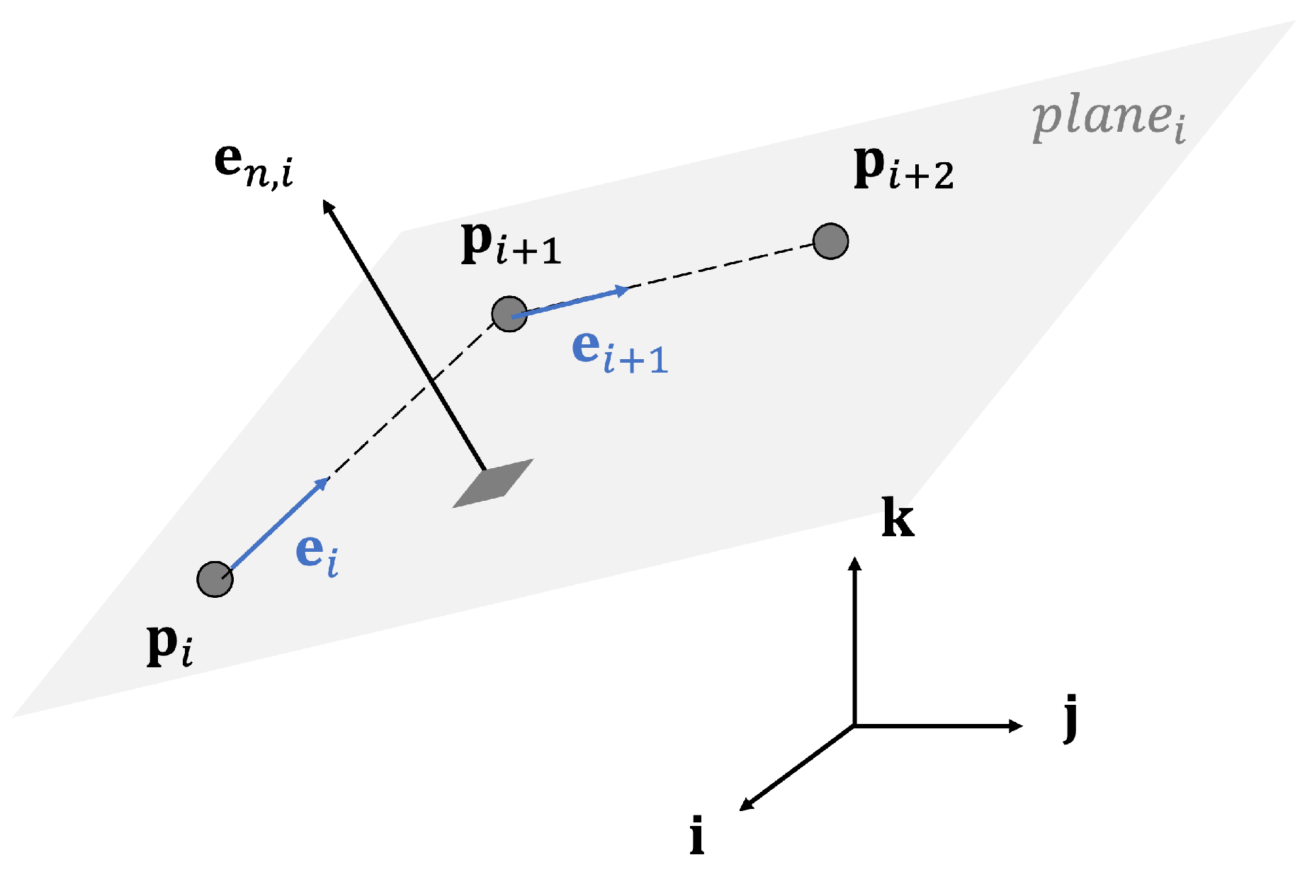
Suppose that is a sequence of waypoints in a 3D space, which might be generated by a path planner or pruner considering obstacle avoidance or other constraints. The problem is to fit these waypoints with the shortest path satisfying the minimum radius of rotation R.
For each waypoint , we define a pose or direction vector as an unit vector pointing to the next waypoint .
At the final waypoint , a direction vector is designated as an approaching angle to the waypoint.
This definition of a direction vector is very natural in the waypoint guidance problem and is the only constraint, which makes it possible to extend a 2D to a 3D Dubins path. In this way, all three sequential waypoint tuples and their associated two-direction vectors are located on the same plane . The consecutive waypoint tuple and their associated direction vectors are also all on another plane . Moreover, the waypoint segment line , which connects the waypoints and , becomes the intersection line of two adjacent planes, and , as shown in Figure 1.
2.1. Two-Dimensional Dubins Path
This subsection describes the 2D Dubins path. Much of this material is found elsewhere but is re-represented using unified vector notation in any plane in 3D space to account for extensions to a 3D path.
For each , four configurations of the conventional 2D Dubins path can be designed with two points and two directions . The four configurations are RSR, RSL, LSR, and LSL, where R is a right turn, L is a left turn, and S is a straight line. The shortest path is chosen by comparing the distance along the Dubins path between two points.
We define a left rotation as a rotation about the unit vector , which is normal to and points the upward direction in a reference frame, as shown in Figure 2.
If and are parallel, the normal vector to is set to the previous one as .
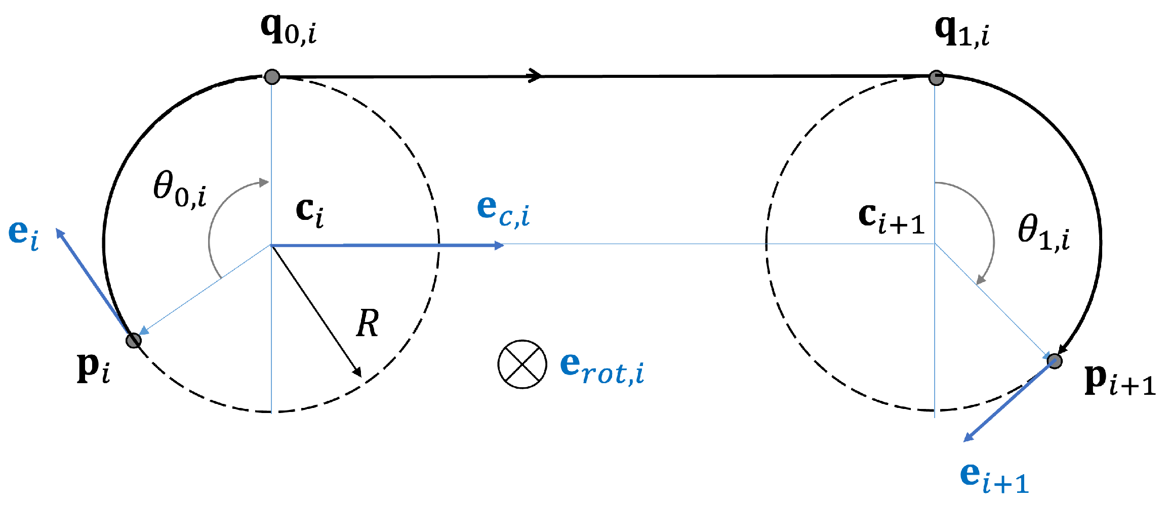
For a given direction vector and the minimum radius of rotation R at waypoint , there are two tangent circular arcs: left and right, as shown in Figure 3. A vehicle can either turn left or right, traversing these circular arcs with the circle’s rotation direction. The centers of both circular arcs are chosen such that the direction vector at waypoint is tangential to both circular arcs and computed as follows:
2.1.1. RSR and LSL
For the RSR case, a trajectory consists of turning right on a right circular arc at waypoint , going straight, and then turning right again on a right arc until the next waypoint is reached. Figure 4 shows the pull-out point at waypoint , which is a transition point from a circular arc to a straight line, and the wheel-over point , which is a transition point from a straight line to a circular arc at waypoint , and a straight line connecting them, respectively.
The pull-out and wheel-over points are computed as follows:
where is the rotation axis of the right circular arc, , , and is an unit direction vector from to .
The rotation angle to traverse from point to is determined by
where
Similarly, the rotation angle to traverse from point to is given as follows:
where
For the LSL case, a trajectory consists of turning left on a left circular arc, going straight, and then turning left again on a left arc until the next waypoint is reached. Figure 5 shows the pull-out and wheel-over points and a straight line connecting them, respectively.
The pull-out, wheel-over points, and rotation angle are computed by the same Equations (4)–(6) with the following replacements:
The distance between two waypoints along the Dubins path is computed by summing the arc lengths along the circumference and straight line.
2.1.2. RSL and LSR
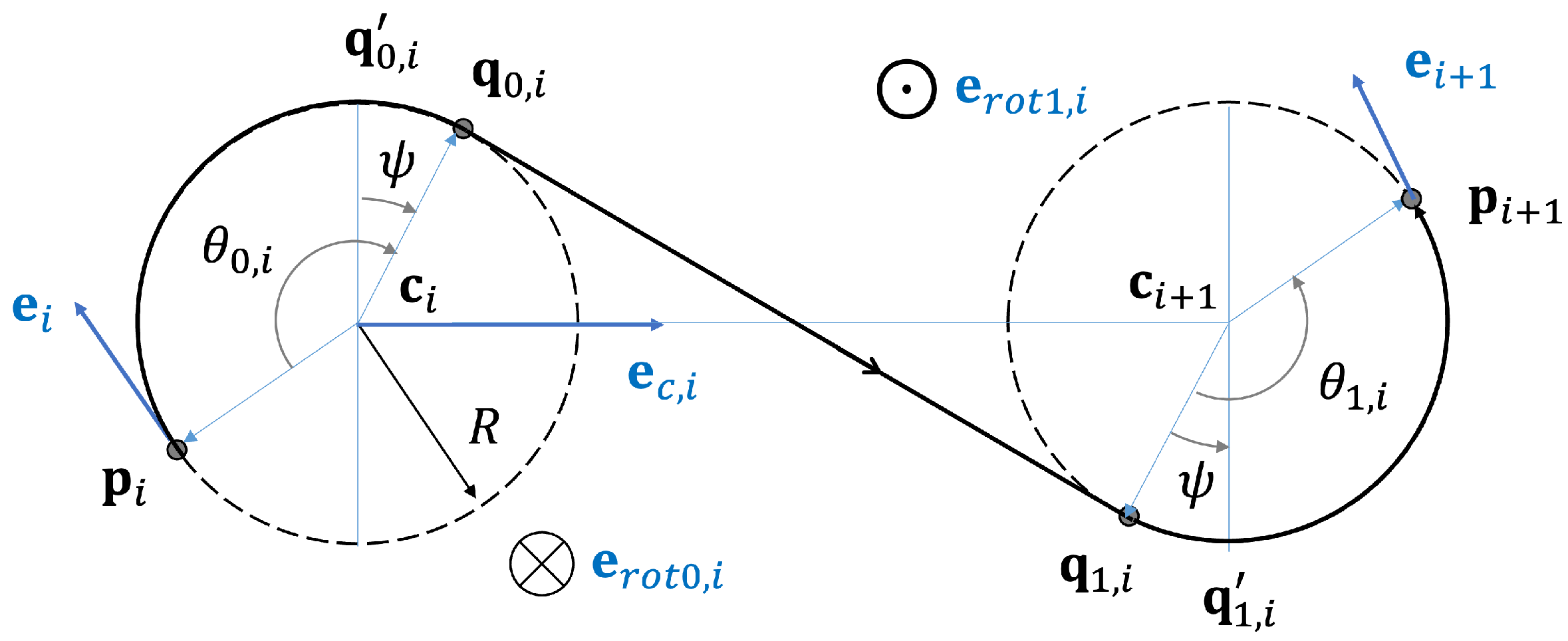
For the RSL case, a trajectory consists of first turning right on a right circular arc at waypoint , going straight, and then turning left on a left arc until the next waypoint is reached. Figure 6 shows the pull-out point , the wheel-over point , and a straight line connecting them, respectively.
The pull-out and wheel-over points are computed as follows:
where
and , are rotation axes, and , are centers of circular arcs.
The rotation angle about the rotation axis to traverse from point to can be determined by
where
Similarly, the rotation angle to traverse from point to is given as follows:
where
For the LSR case, a trajectory consists of first turning left on a left circular arc, followed by straight, and turning right on a right arc until the next waypoint is reached. Figure 7 shows the pull-out and wheel-over points and a straight line connecting them, respectively.
The pull-out, wheel-over points, and rotation angle are computed by the same Equations (9)–(12) with the following replacements:
The distance between two waypoints along the Dubins path is computed as follows:
2.2. Three-Dimensional Dubins Path
A direction vector at each waypoint is defined as the direction to the next waypoint. With this definition, three sequential waypoint tuples and their associated two-direction vectors are all on the same plane , and the next consecutive waypoint tuple and their associated directions are also located on another plane . The is tilted from about the waypoint segment line as amount of .
Because the waypoint segment line is the intersection line of both planes, the circular arcs on and have the same tangent at the waypoint , which is a direction vector along the segment line. Therefore, the Dubins path on both planes is smoothly connected at the waypoint , as shown in Figure 8. This is how to extend the 2D Dubins path to a 3D path in our method.
The advantage of the proposed method is that the problem of the 3D Dubins path becomes just designing 2D Dubins paths on every plane, and the smooth connection between adjacent planes is automatically achieved. This way, it preserves the same complexity and the shortest path property of the 2D Dubins path.
3. Smoothing Methodology
3.1. Cubic Bezier Curve
A cubic Bezier curve is a continuous curvature curve with the smallest order and is given by
where are control points. This curve passes through points and , and passes closely through the two middle points and . Now, suppose that all four control points are on the same plane, and three of them are on the same straight line, i.e.,
where and are unit direction vectors, and and denote the separation distances between control points. The curvature equation of the curve is given by
The curvature is computed as at and is monotonically increasing as t goes. For the curvature to be maximized at with its derivative zero, the separation distance must have the following values, as in [7]:
where L is a design parameter that can be expressed as a function of the maximum allowed curvature, and is the angle between and . The maximum curvature occurs at and is computed as
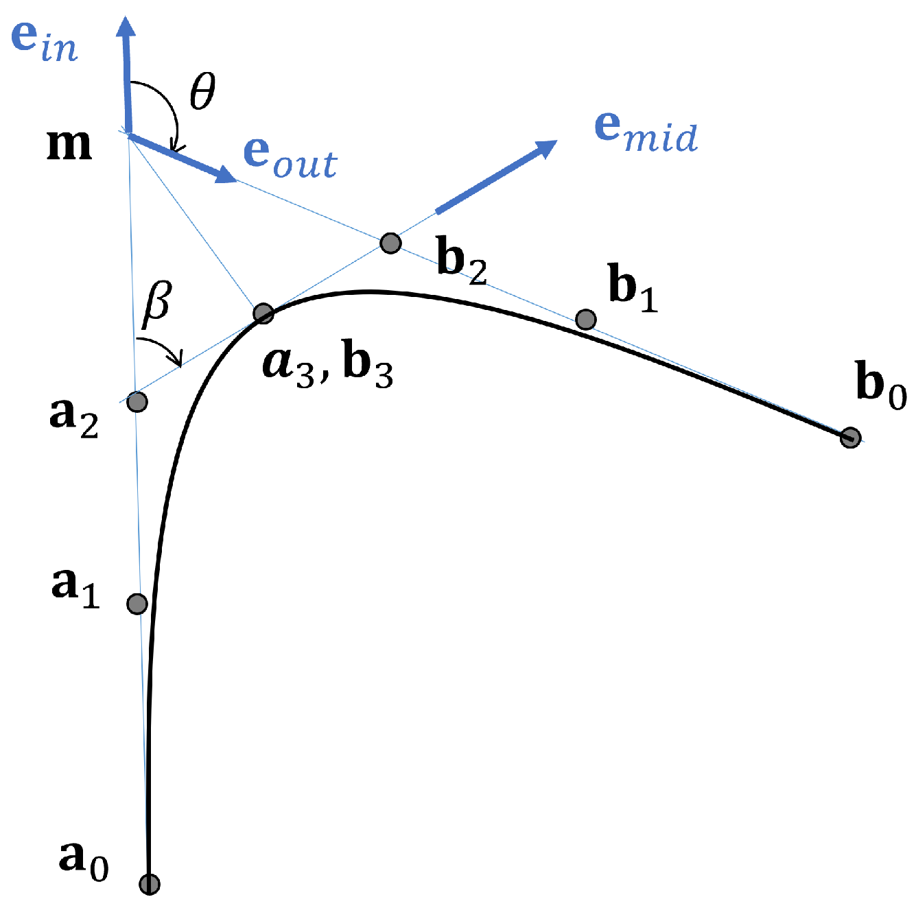
With the Bezier curve described above, two curves can be concatenated to generate a continuous curvature path between two successive line segments in which the curvature is zero at both the start and end points located on each line segment. For two Bezier curves to be connected smoothly and to make maximum curvature occur at the connecting point, the last and first controls of both curves must coincide, and their derivatives of the curvature must be zero.
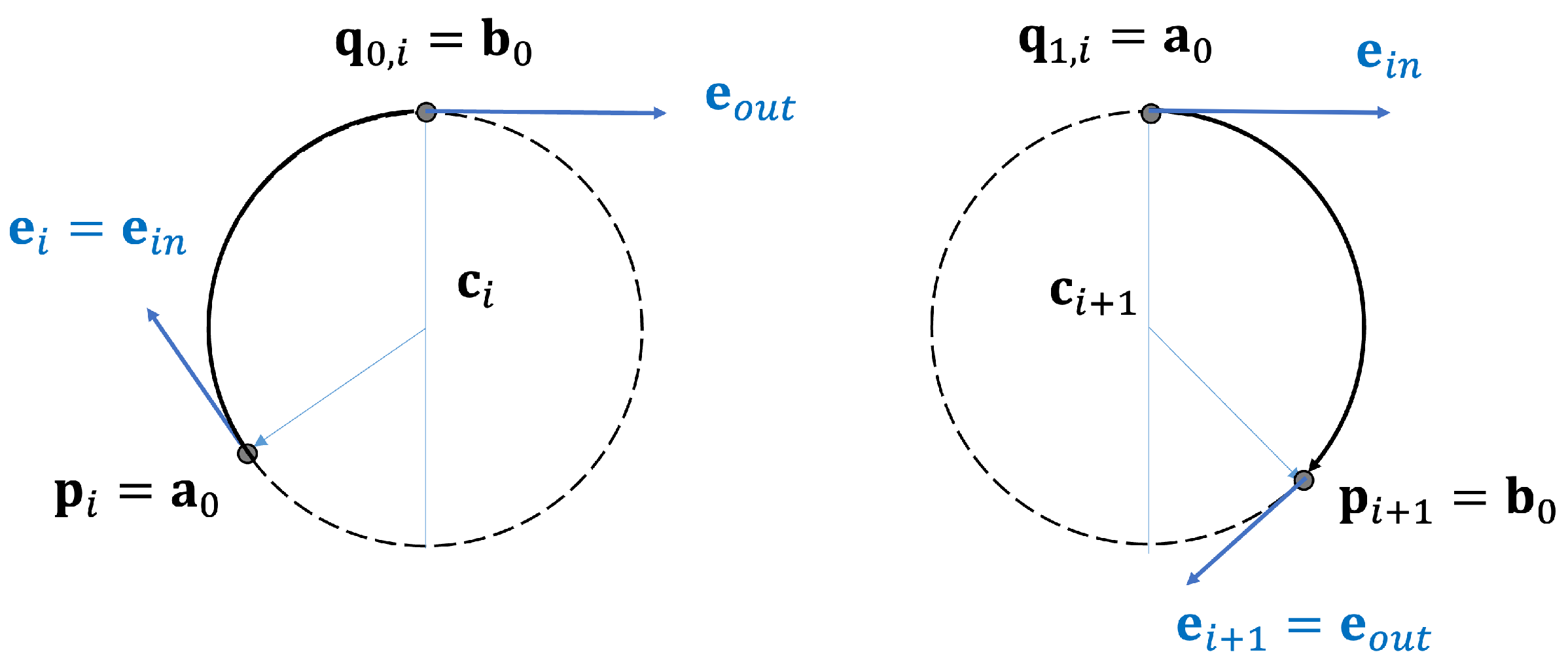
The first Bezier curve and its control points are defined by (15) and (16), and the second curve is defined symmetrically, as shown in Figure 9.
where are control points and defined by the same way to their corresponding counter parts .
In Figure 9, and are unit vectors representing the direction along each line segment, is a unit vector along the line connecting and , is the intersection point of two line segments, and is the turning angle between and , which is by the geometric relationship. It is easily shown that L is a distance from intersection point to or . Points and are located in the center of the line connecting and . The control points and are connecting points and must be equal. The maximum curvature occurs at and , and its value is given by (19). The curvatures at and are, respectively, zero.
In summary, two concatenated Bezier curves produce a circular arc-like curve with maximum curvature at the middle point and zero curvature at the start and end points.
3.2. Dubins Path Approximation
Our goal is to construct a 3D path with continuous curvature for given multiple waypoints that all must be passed through. Although the proposed 3D Dubins path algorithm produces the shortest path in 3D space, its curvature is discontinuous at the transition point between a straight line and a circular arc. Since the cubic Bezier curve is a G2-continuous curvature curve, it can be used as a transition curve between a straight line and a circular arc of Dubins path to make a smooth connection.
In this paper, we propose a 3D Dubins-path-guided continuous curvature path-smoothing algorithm using the cubic Bezier curve. The proposed algorithm generates a parametric path that simultaneously satisfies curvature continuity and maximum curvature requirements.
Once the 3D Dubins path is designed, the pull-out and wheel-over points and their direction vectors are determined, which are the transition points where a straight line and a circular arc meet. The angle between two-direction vectors at the waypoint and its corresponding pull-out or wheel-over point, i.e., the turning angle , can also be computed.
In the case of a circular arc departure, if a waypoint and a pull-out point are assigned as a control point and in (15) and (20), respectively, the circular arc can be approximated as a Bezier curve. Similarly, if a wheel-over point and a waypoint are assigned as a control point and , respectively, the circular arc can also be approximated as a Bezier curve in a case of arrival, as shown in Figure 10. Since the Bezier curve passes through points and , all waypoints are guaranteed to pass through.
Different from the conventional Bezier curve design, a design parameter L in (18), which is selected considering maximum allowable curvature, is now computed as a function of turning angle in our method.
where is a waypoint and is a corresponding pull-out or wheel-over point. With the computed L, the maximum curvature is also determined from (19) and (22) as
The problem is that the calculated maximum curvature is always greater than the maximum permissible curvature constraint, and this tendency worsens as the turning angle provided by the Dubins path increases. Moreover, a Bezier curve is possible only when the turning angle is less than 180 degrees.
Because the maximum curvature is calculated only with a turning angle, the turning angle must be reduced to much less than 180 degrees to reduce the maximum curvature and overcome the limitation of the Bezier curve. In this paper, we propose to divide the circular arc into several parts and approximate each piece with a Bezier curve until the approximation curve does not deviate too far from the circular arc and the maximum permissible curvature constraint.
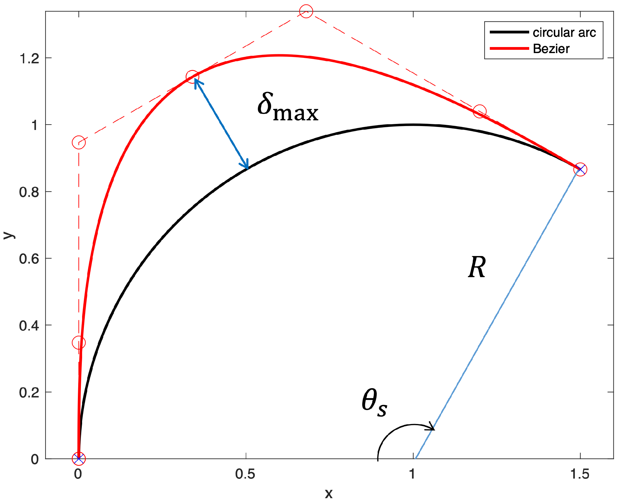
The maximum curvature and the largest deviation occur at the midpoint of the split circular arc and are, respectively, given as follows:
where is the split turning angle. Figure 11 represents the largest deviation and split turning angle .
The reasonable value for can be chosen based on (24). For example, and at are computed as follows:
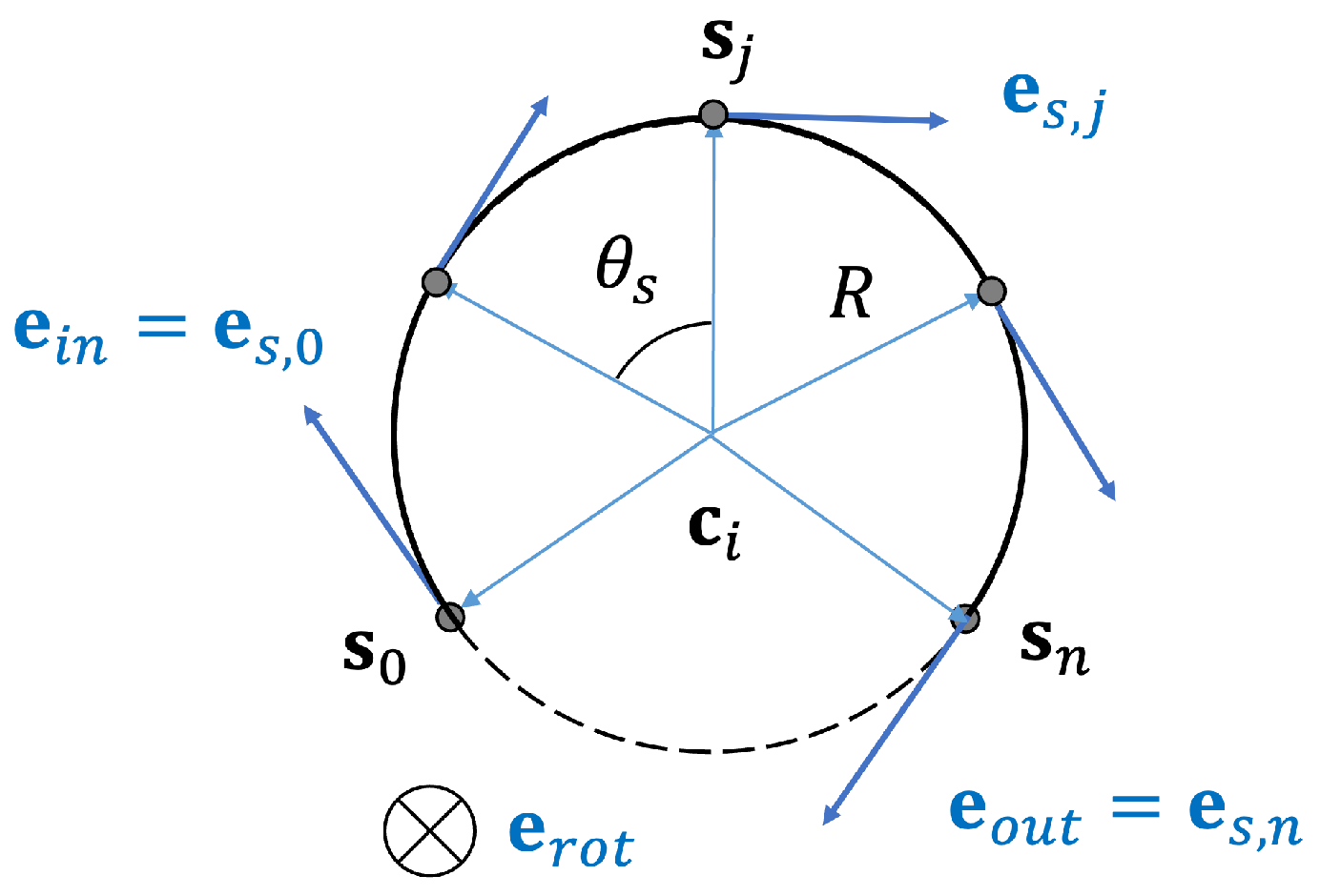
Once the split turning angle is selected, the circular arc is split evenly into n segments, as shown in Figure 12, where and are consecutive start and end points of the segmented arc. In the case of a circular arc departure, and , while in the case of arrival, and .
The position and direction vector of a specific point on the circular arc in Figure 12 can be easily calculated by the following equations:
where and .
Figure 13 shows an example of a circular arc with a turning angle of 150 degrees. Here, the left figure shows an approximation with one Bezier curve and the right figure one with five Bezier curves. Comparing the figure on the right with the figure on the left, it can be seen that the Bezier curve hardly differs from the circular arc, and the curvature is significantly reduced.
To strictly meet the maximum curvature requirement, the radius of the circular arc should be slightly increased when designing the Dubins reference path for the Bezier curve approximation.
4. Simulations
The numerical simulations are conducted to evaluate the proposed path-smoothing algorithm. In the simulations, two sequences of waypoints are considered, as shown in Table 1 and Table 2. The turning radius of the vehicle is set to R = 30 m, which corresponds to the maximum curvature constraint of . In the first waypoint sequence, the waypoints are far away relative to the turning radius, but the second is not. The approaching direction to the final waypoint of both sequences is assumed to be the direction. Considering (24) or (25), when designing a Dubins reference path for Bezier curve approximation, the split turning angle is chosen as and the base radius of the angular arc as = 34.872 m to meet the maximum curvature constraint.
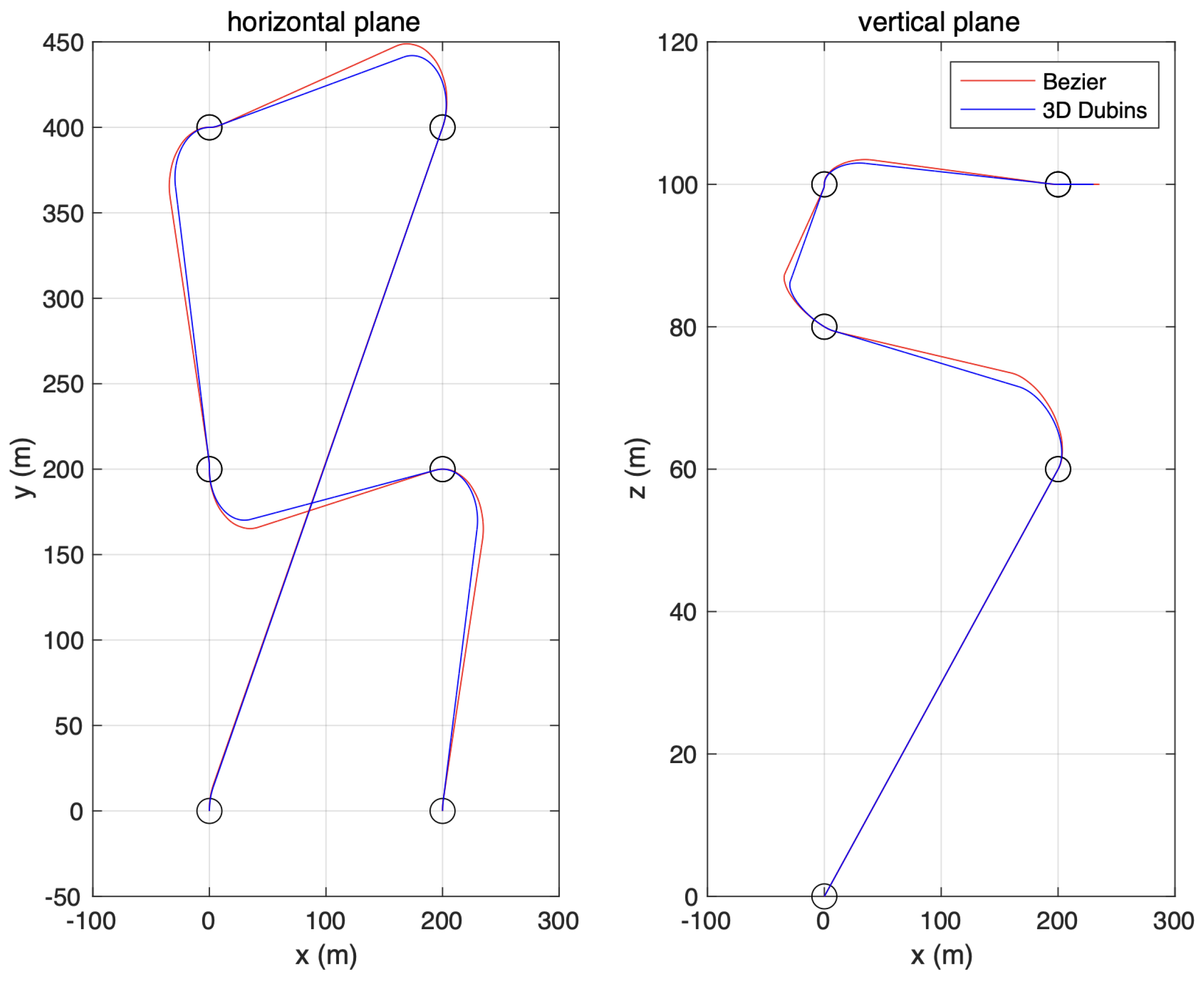
The Dubins path and Bezier curve approximation path are generated from a series of waypoints in Table 1, as shown in Figure 14, and the horizontal and vertical plan views are shown in Figure 15. From the figures, it can be seen that both paths pass through all waypoints marked with ’o’.
Note that the Dubins path and Dubins reference path are different. The Dubins reference path is for designing Bezier curve approximation, and it is created by adjusting the circular arc radius as , whereas the Dubins path is designed with radius R. Therefore, the trajectory difference seen in the figures should not be interpreted as trajectory estimation error.
The Dubins path consists of the following sequence: RSL, LSR, LSR, LSR, and RSL, and has a length of 1351.5 m. The length of the Bezier curve approximation is 1371.0 m, which is a 19.5 m increase. However, the curvature of the Dubins path is discontinuous at the transition points, since the path directly transitions from line segments to circular arcs. In contrast, the Bezier curve approximation is a continuous curvature path satisfying maximum curvature constraints, as shown in Figure 16. The horizontal dashed line in the figure indicates the maximum curvature limit. The Bezier curve approximation is, therefore, a feasible path.
Figure 17 is a partially enlarged view of Figure 16. It shows that the circular arc segment of the Dubins path is approximated by several Bezier curves to meet the maximum curvature requirement.
For the sequence of waypoints in Table 2, the Dubins path and its Bezier curve approximation are shown in Figure 18 and Figure 19. The Dubins path and its approximated Bezier paths look complicated because the waypoints are relatively close to the turning radius. However, both paths pass through all waypoints. The Dubins path consists of the following sequence: LSL, RSR, RSL, RSL, and RSL, and has a length of 1042.6 m. The length of the Bezier curve approximation is 1196.8 m, which is a 154.2 m increase. The length of the Bezier curve approximation is a bit longer due to the large portion of the circular arc segment of the Dubins path.
Figure 20 is the curvature plot of both paths, showing that only the Bezier curve approximation has continuous curvature and satisfies the maximum curvature requirement.
5. Conclusions
In this paper, we present a novel smoothing algorithm generating a three-dimensional continuous curvature path from a sequence of waypoints. Our algorithm is composed of two stages: one is a reference path generation by the 3D Dubins path, and the other is a reference path approximation by several cubic Bezier curves.
For the 3D Dubins reference path, we propose a novel method to extend a 2D Dubins path to a 3D path by applying a simple constraint that the pose is a unit vector pointing to the next waypoint to the pose of each waypoint. Our method is straightforward for use in waypoint guidance problems. Its advantages include preserving the same methodology and complexity of the 2D Dubins path design.
Since the curvature of the resulting 3D Dubins reference path is discontinuous at the transition point between a straight line and a circular arc, we propose to divide the circular arc into several parts and approximate each piece using a Bezier curve to avoid curvature discontinuity. This method also overcomes the limitation on the size of the turning angle of the Bezier curve and allows all waypoints to pass through. We also provide a criterion to select a required number of Bezier curves to strictly meet the maximum curvature constraint.
The numerical simulations are conducted to evaluate the proposed path-smoothing algorithm. In the simulations, two different sequences of waypoints are considered. The results show that the proposed algorithm produces a continuous curvature path that passes through all waypoints with a slight increase in path length compared with the Dubins reference path.
Our path-smoothing algorithm can be used for path following applications in many areas, such as aerospace and robotics, as it generates a 3D parametric path that simultaneously satisfies curvature continuity and maximum curvature requirements. However, since the proposed algorithm is tested only in simulation and not in a real environment, future work will be to perform experiments in a real environment.
Funding
This work was supported by the National Research Foundation of Korea (NRF) grant funded by the Korea government (MSIT) (NRF-2021R1F1A1063780).
Institutional Review Board Statement
Not applicable.
Informed Consent Statement
Not applicable.
Data Availability Statement
Not applicable.
Conflicts of Interest
The author declares no conflict of interest.
References
- Elbanhawi, M.; Simic, M. Sampling-Based Robot Motion Planning: A Review. IEEE Access 2014, 2, 56–77. [Google Scholar] [CrossRef]
- Amato, N.; Bayazit, O.; Dale, L.; Jones, C.; Vallejo, D. Choosing good distance metrics and local planners for probabilistic roadmap methods. IEEE Trans. Robot. Autom. 2000, 16, 442–447. [Google Scholar] [CrossRef]
- Ahmad, Z.; Ullah, F.; Tran, G.; Lee, S. Efficient Energy Flight Path Planning Algorithm Using 3-D Visibility Roadmap for Small Unmanned Aerial Vehicle. Int. J. Aerosp. Eng. 2017, 2017, 2849745. [Google Scholar] [CrossRef] [Green Version]
- Lee, D.; Shim, D. Spline-RRT* Based Optimal Path Planning of Terrain Following Flights for Fixed-Wing UAVs. In Proceedings of the International Conference on URAI, Kuala Lumpur, Malaysia, 12–15 November 2014. [Google Scholar]
- Tsai, Y.; Lee, C.; Lin, C.; Huang, C. Development of Flight Path Planning for Multirotor Aerial Vehicles. Aerospace 2015, 2, 171–188. [Google Scholar] [CrossRef] [Green Version]
- Yang, Y.; Sukkarieh, S. 3D Smooth Path Planning for a UAV in Cluttered NaturalEnvironments. In Proceedings of the International Conference on Intelligent Robotics and Systems, Nice, France, 22–26 September 2008. [Google Scholar]
- Yang, K.; Sukkarieh, S. An Analytical Continuous-Curvature Path-Smoothing Algorithm. IEEE Trans. Robot. 2010, 26, 561–568. [Google Scholar] [CrossRef]
- Ravankar, A.; Ravankar, A.A.; Kobayashi, Y.; Hoshino, Y.; Peng, C. Path Smoothing Techniques in Robot Navigation: State-of-the-Art, Current and Future Challenges. Sensors 2018, 18, 3170. [Google Scholar] [CrossRef] [PubMed] [Green Version]
- Cimurs, R.; Suh, I. Time-optimized 3D Path Smoothing with Kinematic Constraints. Int. J. Control Autom. Syst. 2020, 18, 1277–1287. [Google Scholar] [CrossRef]
- Ahmed, A.; Soliman, A.; Maged, A.; Gaafar, M.; Magdy, M. Path Smoothing Algorithm Using Thin-Plate Spline. In Proceedings of the 7th International Conference on Control, Automation and Robotics, Singapore, 3–26 April 2021. [Google Scholar]
- Dubins, L. On curves of minimal length with a constraint on average curvature, and with prescribed initial and terminal positions and tangents. Am. J. Math. 1957, 79, 497–516. [Google Scholar] [CrossRef]
- Cardenas, I.; Flores, G.; Salazar, S.; Lo, R. Dubins Path Generation for a Fixed Wing UAV. In Proceedings of the International Conference on Unmanned Aircraft Systems, Orlando, FL, USA, 27–30 May 2014. [Google Scholar]
- Tsourdos, A.; White, B.; Shanmugavel, M. Path Planning in Three Dimensions. In Cooperative Path Planning of Unmanned Aerial Vehicles; Wiley: Chichester, West Sussex, UK, 2011; pp. 65–78. [Google Scholar]
- Vana, P.; Neto, A.; Faigl, J.; Macharet, D. Minimal 3D Dubins Path with Bounded Curvature and Pitch Angle. In Proceedings of the IEEE International Conference on Robotics and Automation, Paris, France, 31 May 2020. [Google Scholar]
- Rognli, V. Path Generation and Spline Approximation of a 3D Extended Dubins Path. Master’s Thesis, Norwegian University of Science and Technology, Trondheim, Norway, 2021. [Google Scholar]
- Cai, W.; Zhang, M. Smooth 3D Dubins Curves Based Mobile Data Gathering in Sparse Underwater Sensor Networks. Sensors 2018, 18, 2105. [Google Scholar] [CrossRef] [PubMed] [Green Version]
- Choi, J.; Curry, R.; Elkaim, G. Continuous Curvature Path Generation Based on Bezier Curves for Autonomous Vehicles. Int. J. Appl. Math. 2010, 40, 91–101. [Google Scholar]
- Lekkas, A.; Dahl, A.; Breivik, M.; Fossen, T. Continuous-Curvature Path Generation Using Fermat’s Spiral. Model. Identif. Control 2013, 34, 183–198. [Google Scholar] [CrossRef]
- Li, F.-F.; Du, Y.; Jia, K.-J. Path planning and smoothing of mobile robot based on improved artifcial fish swarm algorithm. Sci. Rep. 2022, 12, 659. [Google Scholar] [CrossRef]
- Shkel, A.; Lumelsky, V. Classification of the Dubins set. Robot. Auton. Syst. 2001, 34, 179–202. [Google Scholar] [CrossRef]
Figure 1.
Waypoints and planes.

Figure 2.
Normal vector to a plane.

Figure 3.
Left and right circle at a waypoint.

Figure 4.
RSR path.

Figure 5.
LSL path.

Figure 6.
RSL path.

Figure 7.
LSR path.

Figure 8.
Two planes and intersection line.

Figure 9.
Two Bezier curves.

Figure 10.
Circular arc approximation.

Figure 11.
Circular arc and Bezier curve approximation.

Figure 12.
Split circular arc.

Figure 13.
Bezier curve approximation for the split circular arc.

Figure 14.
Three-dimensional Dubins path and Bezier approximation.

Figure 15.
Horizontal and vertical plan views.

Figure 16.
Curvature.

Figure 17.
Partially enlarged view of Figure 16.
Figure 17.
Partially enlarged view of Figure 16.

Figure 18.
Three-dimensional Dubins path and Bezier approximation.

Figure 19.
Horizontal and vertical plan views.

Figure 20.
Curvature.


Table 1.
Waypoints I.
| Coordinate | Waypoints | |||||
|---|---|---|---|---|---|---|
| #1 | #2 | #3 | #4 | #5 | #6 | |
| 200 | 200 | 0 | 0 | 200 | 0 | |
| 0 | 200 | 200 | 400 | 400 | 0 | |
| 100 | 100 | 100 | 80 | 60 | 0 | |
Table 2.
Waypoints II.
| Coordinate | Waypoints | |||||
|---|---|---|---|---|---|---|
| #1 | #2 | #3 | #4 | #5 | #6 | |
| 20 | 20 | 0 | 0 | 20 | 0 | |
| 0 | 20 | 20 | 40 | 40 | 0 | |
| 100 | 100 | 100 | 80 | 60 | 0 | |
Publisher’s Note: MDPI stays neutral with regard to jurisdictional claims in published maps and institutional affiliations. |
© 2022 by the author. Licensee MDPI, Basel, Switzerland. This article is an open access article distributed under the terms and conditions of the Creative Commons Attribution (CC BY) license (https://creativecommons.org/licenses/by/4.0/).
Share and Cite
MDPI and ACS Style
Park, S. Three-Dimensional Dubins-Path-Guided Continuous Curvature Path Smoothing. Appl. Sci. 2022, 12, 11336. https://doi.org/10.3390/app122211336
AMA Style
Park S. Three-Dimensional Dubins-Path-Guided Continuous Curvature Path Smoothing. Applied Sciences. 2022; 12(22):11336. https://doi.org/10.3390/app122211336
Chicago/Turabian StylePark, Sungsu. 2022. "Three-Dimensional Dubins-Path-Guided Continuous Curvature Path Smoothing" Applied Sciences 12, no. 22: 11336. https://doi.org/10.3390/app122211336
Note that from the first issue of 2016, this journal uses article numbers instead of page numbers. See further details here.