

Cascaded Reinforcement Learning Agents for Large Action Spaces in Autonomous Penetration Testing
 , , , and
Abstract
:1. Introduction
2. Related Work
3. Background
4. Methodology
4.1. Algebraic Action Decomposition Scheme
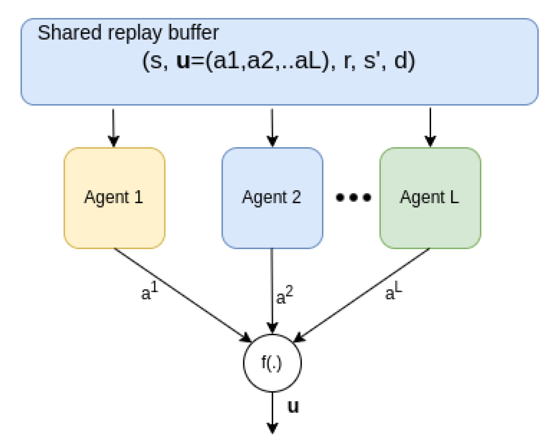
4.2. Cooperative Multi-Agent Training
4.3. CRLA Implementation
4.4. Algorithms Pseudocode
| Algorithm 1 CRLA—Cascaded Reinforcement Learning Agents |
|
| Algorithm 2 Initialise the agents |
|
5. Experiment Setup
5.1. Toy Maze Scenario
5.2. The CybORG Simulator
5.3. Neural Network Architecture
6. Results
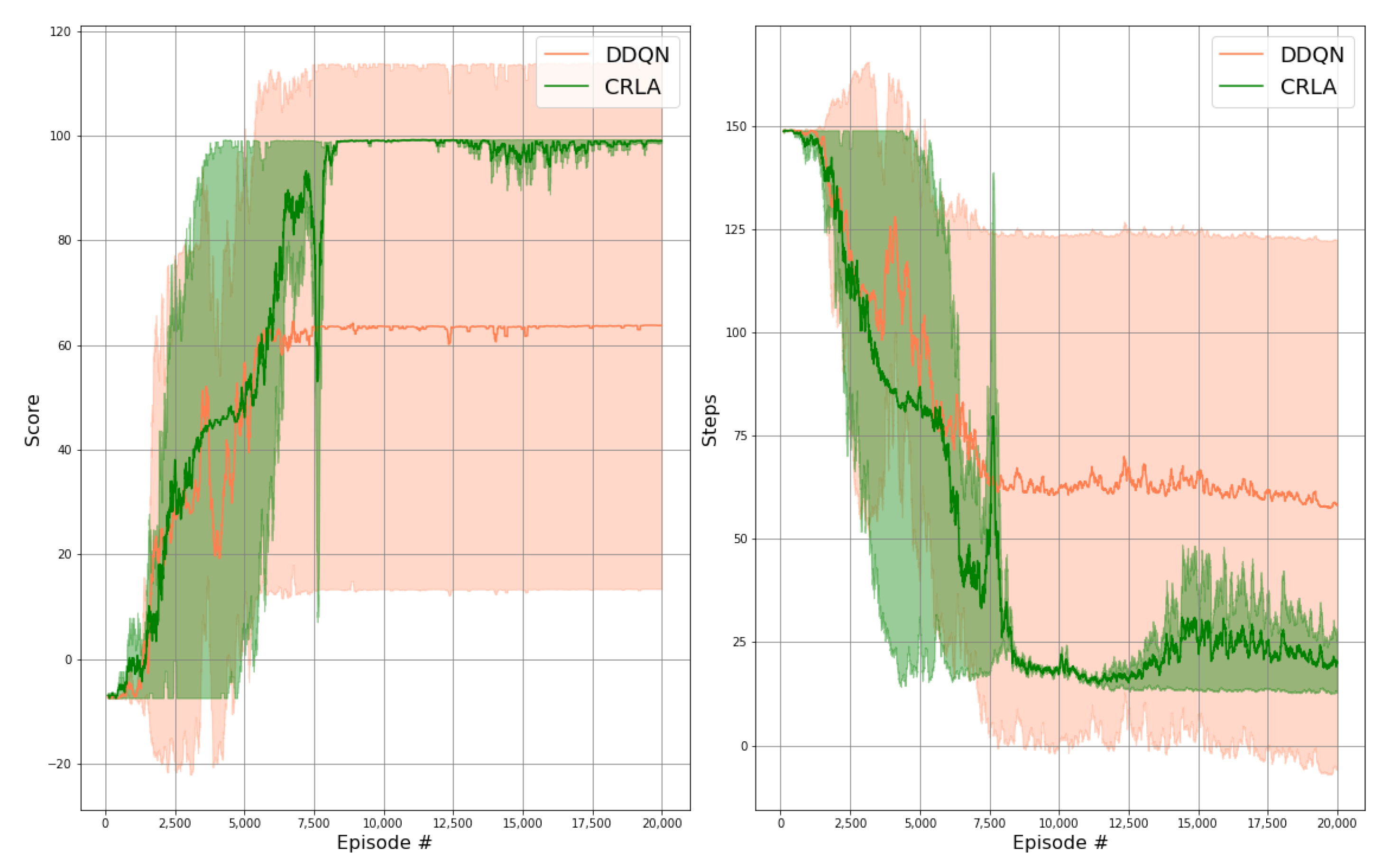
6.1. Maze
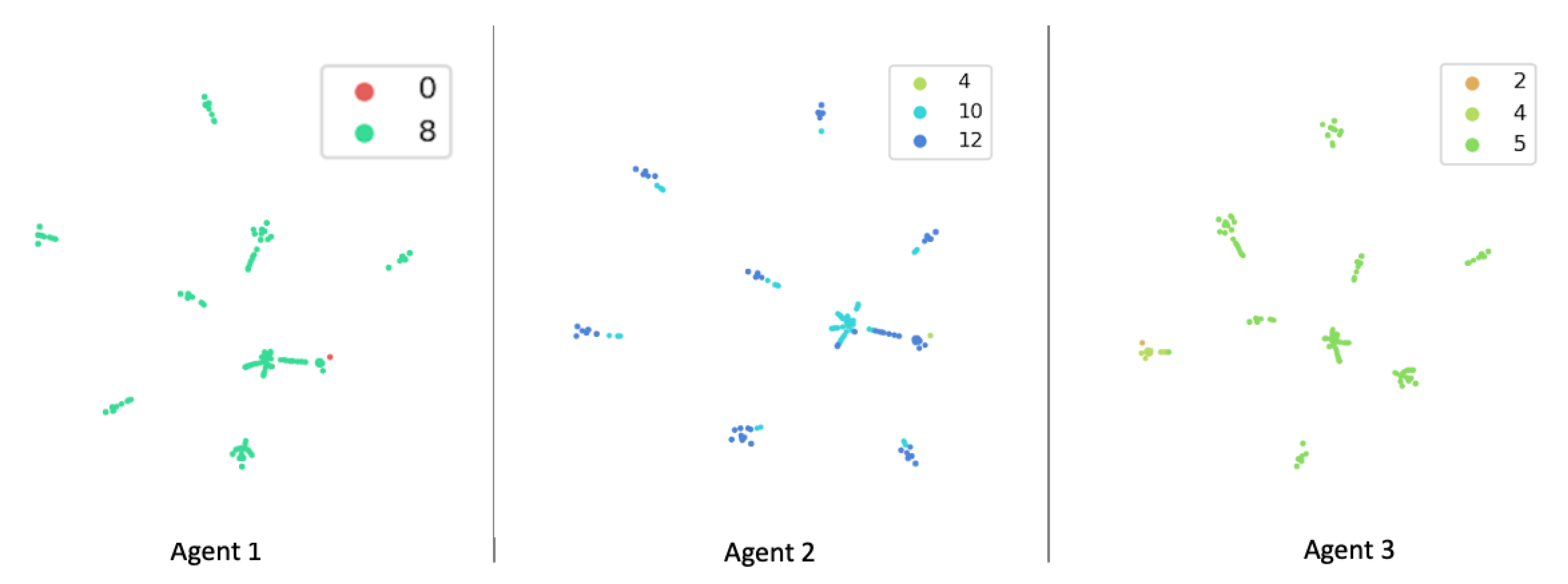
6.2. CybORG
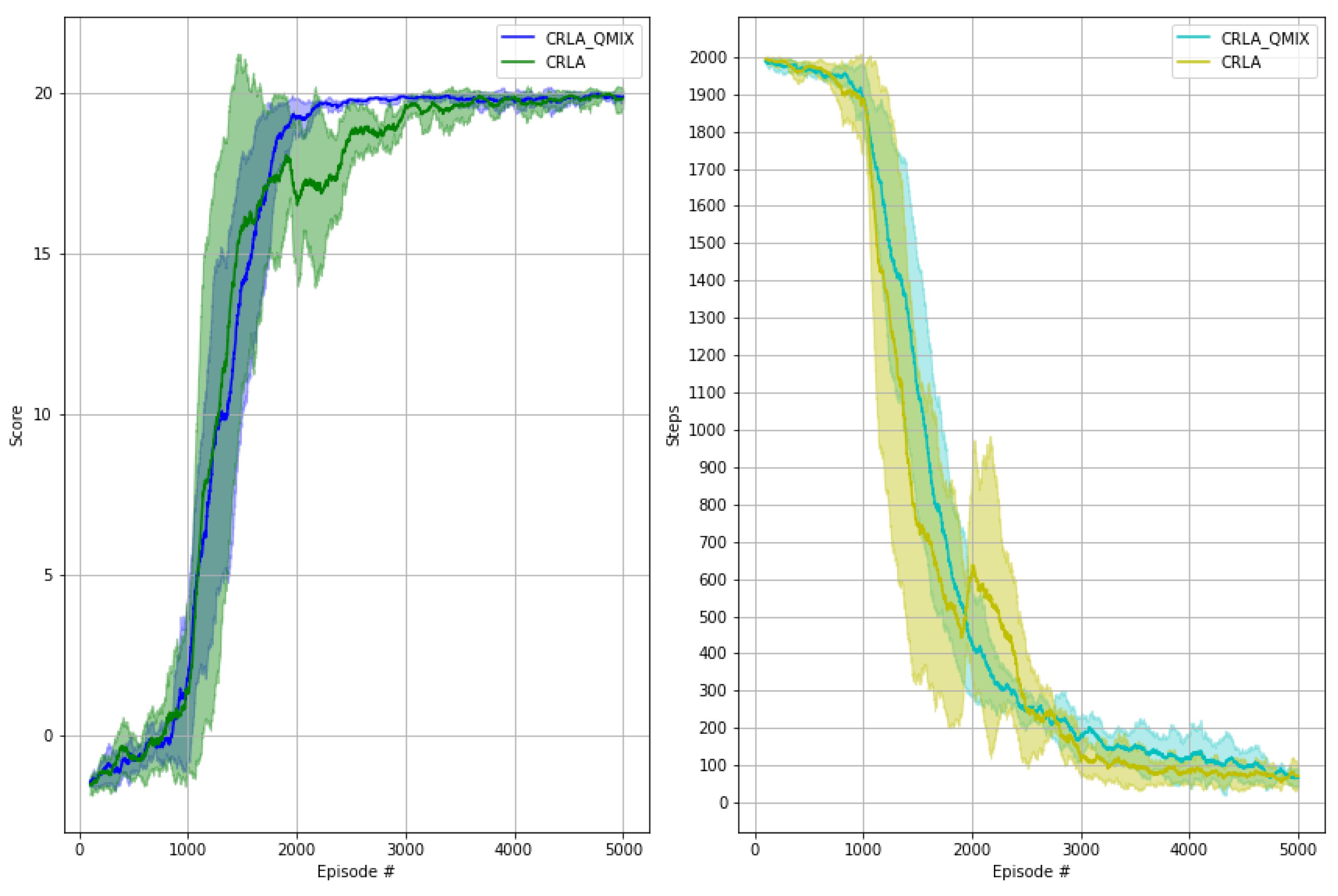
6.3. Cooperative Learning with QMIX
6.4. Discussion
7. Conclusions
Author Contributions
Funding
Conflicts of Interest
Abbreviations
| CRLA | Cascaded reinforcement learning agents |
| MDP | Markov decision process |
| POMDP | Partially observable MDP |
| RL | Reinforcement learning |
| CybORG | Cyber Operations Research Gym |
| DQN | Deep Q-network |
| GPU | Graphical processing unit |
Appendix A. Network Comparison

References
- Mnih, V.; Kavukcuoglu, K.; Silver, D.; Rusu, A.A.; Veness, J.; Bellemare, M.G.; Graves, A.; Riedmiller, M.; Fidjeland, A.K.; Ostrovski, G.; et al. Human-level control through deep reinforcement learning. Nature 2015, 518, 529. [Google Scholar] [CrossRef] [PubMed]
- Lillicrap, T.P.; Hunt, J.J.; Pritzel, A.; Heess, N.; Erez, T.; Tassa, Y.; Silver, D.; Wierstra, D. Continuous control with deep reinforcement learning. arXiv 2015, arXiv:1509.02971. [Google Scholar]
- Watkins, C.J.; Dayan, P. Q-learning. Mach. Learn. 1992, 8, 279–292. [Google Scholar] [CrossRef]
- Wang, Z.; Schaul, T.; Hessel, M.; Van Hasselt, H.; Lanctot, M.; De Freitas, N. Dueling network architectures for deep reinforcement learning. arXiv 2015, arXiv:1511.06581. [Google Scholar]
- Hessel, M.; Modayil, J.; van Hasselt, H.; Schaul, T.; Ostrovski, G.; Dabney, W.; Horgan, D.; Piot, B.; Azar, M.G.; Silver, D. Rainbow: Combining Improvements in Deep Reinforcement Learning. In Proceedings of the Thirty-second AAAI conference on artificial intelligence 2018, New Orleans, LA, USA, 2–7 February 2018. [Google Scholar]
- Fan, J.; Wang, Z.; Xie, Y.; Yang, Z. A Theoretical Analysis of Deep Q-Learning. In Proceedings of Machine Learning Research, Proceedings of the 2nd Conference on Learning for Dynamics and Control, Berkeley, CA, USA, 11–12 June 2020; Bayen, A.M., Jadbabaie, A., Pappas, G., Parrilo, P.A., Recht, B., Tomlin, C., Zeilinger, M., Eds.; ML Research Press: Maastricht, The Netherlands, 2020; Volume 120, pp. 486–489. [Google Scholar]
- Farquhar, G.; Gustafson, L.; Lin, Z.; Whiteson, S.; Usunier, N.; Synnaeve, G. Growing Action Spaces. In Proceedings of the International Conference on Machine Learning 2020, Virtual, 24–26 November 2020. [Google Scholar]
- Schwartz, J.; Kurniawati, H. Autonomous Penetration Testing using Reinforcement Learning. arXiv 2019, arXiv:cs.CR/1905.05965. [Google Scholar]
- Tavakoli, A.; Pardo, F.; Kormushev, P. Action branching architectures for deep reinforcement learning. In Proceedings of the Thirty-Second AAAI Conference on Artificial Intelligence, New Orleans, LA, USA, 2–7 February 2018. [Google Scholar]
- Dulac-Arnold, G.; Evans, R.; van Hasselt, H.; Sunehag, P.; Lillicrap, T.; Hunt, J.; Mann, T.; Weber, T.; Degris, T.; Coppin, B. Deep reinforcement learning in large discrete action spaces. arXiv 2015, arXiv:1512.07679. [Google Scholar]
- Standen, M.; Lucas, M.; Bowman, D.; Richer, T.J.; Kim, J.; Marriott, D. CybORG: A Gym for the Development of Autonomous Cyber Agents. arXiv 2021, arXiv:2108.09118. [Google Scholar]
- Hu, Z.; Beuran, R.; Tan, Y. Automated Penetration Testing Using Deep Reinforcement Learning. In Proceedings of the 2020 IEEE European Symposium on Security and Privacy Workshops (EuroS&PW), Genoa, Italy, 7–11 September 2020; pp. 2–10. [Google Scholar]
- Zennaro, F.M.; Erdodi, L. Modeling penetration testing with reinforcement learning using capture-the-flag challenges and tabular Q-learning. arXiv 2020, arXiv:2005.12632. [Google Scholar]
- Zahavy, T.; Haroush, M.; Merlis, N.; Mankowitz, D.J.; Mannor, S. Learn What Not to Learn: Action Elimination with Deep Reinforcement Learning. In Proceedings of the Advances in Neural Information Processing Systems, Montreal, QC, Canada, 3–8 December 2018. [Google Scholar]
- Chandak, Y.; Theocharous, G.; Kostas, J.; Jordan, S.M.; Thomas, P.S. Learning Action Representations for Reinforcement Learning. In Proceedings of the International Conference on Machine Learning 2019, Long Beach, CA, USA, 10–15 June 2019. [Google Scholar]
- de Wiele, T.V.; Warde-Farley, D.; Mnih, A.; Mnih, V. Q-Learning in enormous action spaces via amortized approximate maximization. arXiv 2020, arXiv:cs.LG/2001.08116. [Google Scholar]
- Rashid, T.; Samvelyan, M.; de Witt, C.S.; Farquhar, G.; Foerster, J.N.; Whiteson, S. QMIX: Monotonic Value Function Factorisation for Deep Multi-Agent Reinforcement Learning. In Proceedings of the International Conference on Machine Learning 2018, Stockholm, Sweden, 10–15 July 2018. [Google Scholar]
- Masson, W.; Konidaris, G.D. Reinforcement Learning with Parameterized Actions. In Proceedings of the Thirtieth AAAI Conference on Artificial Intelligence 2016, Phoenix, AZ, USA, 12–17 February 2016. [Google Scholar]
- Fan, Z.; Su, R.; Zhang, W.; Yu, Y. Hybrid Actor-Critic Reinforcement Learning in Parameterized Action Space. arXiv 2019, arXiv:1903.01344. [Google Scholar]
- Tan, M. Multi-Agent Reinforcement Learning: Independent versus Cooperative Agents. In Proceedings of the Tenth International Conference on Machine Learning (ICML 1993), Amherst, MA, USA, 27–29 July 1993; pp. 330–337. [Google Scholar]
- Leibo, J.Z.; Zambaldi, V.F.; Lanctot, M.; Marecki, J.; Graepel, T. Multi-agent Reinforcement Learning in Sequential Social Dilemmas. arXiv 2017, arXiv:1702.03037. [Google Scholar]
- Sunehag, P.; Lever, G.; Gruslys, A.; Czarnecki, W.M.; Zambaldi, V.F.; Jaderberg, M.; Lanctot, M.; Sonnerat, N.; Leibo, J.Z.; Tuyls, K.; et al. Value-Decomposition Networks For Cooperative Multi-Agent Learning. arXiv 2017, arXiv:1706.05296. [Google Scholar]
- Ha, D.; Dai, A.M.; Le, Q.V. HyperNetworks. arXiv 2016, arXiv:1609.09106. [Google Scholar]
- Paszke, A.; Gross, S.; Chintala, S.; Chanan, G.; Yang, E.; DeVito, Z.; Lin, Z.; Desmaison, A.; Antiga, L.; Lerer, A. Automatic differentiation in PyTorch. In Proceedings of the NIPS 2017 Autodiff Workshop, Long Beach, CA, USA, 9 December 2017. [Google Scholar]
- Ghanem, M.C.; Chen, T.M. Reinforcement Learning for Efficient Network Penetration Testing. Information 2020, 11, 6. [Google Scholar] [CrossRef] [Green Version]
- Van der Maaten, L.; Hinton, G. Visualizing data using t-SNE. J. Mach. Learn. Res. 2008, 9, 2579–2605. [Google Scholar]


| Hosts | State Space | Action Space | Number of Agents |
|---|---|---|---|
| 6 | 39 | 49 | 2 |
| 9 | 55 | 120 | 2 |
| 12 | 71 | 182 | 2 |
| 18 | 217 | 342 | 2 |
| 24 | 285 | 550 | 2 |
| 50 | 573 | 1326 | 3 |
| 60 | 685 | 1830 | 4 |
| 70 | 797 | 2414 | 4 |
| 100 | 1133 | 4646 | 4 |
Publisher’s Note: MDPI stays neutral with regard to jurisdictional claims in published maps and institutional affiliations. |
© 2022 by the authors. Licensee MDPI, Basel, Switzerland. This article is an open access article distributed under the terms and conditions of the Creative Commons Attribution (CC BY) license (https://creativecommons.org/licenses/by/4.0/).
Share and Cite
Tran, K.; Standen, M.; Kim, J.; Bowman, D.; Richer, T.; Akella, A.; Lin, C.-T. Cascaded Reinforcement Learning Agents for Large Action Spaces in Autonomous Penetration Testing. Appl. Sci. 2022, 12, 11265. https://doi.org/10.3390/app122111265
Tran K, Standen M, Kim J, Bowman D, Richer T, Akella A, Lin C-T. Cascaded Reinforcement Learning Agents for Large Action Spaces in Autonomous Penetration Testing. Applied Sciences. 2022; 12(21):11265. https://doi.org/10.3390/app122111265
Chicago/Turabian StyleTran, Khuong, Maxwell Standen, Junae Kim, David Bowman, Toby Richer, Ashlesha Akella, and Chin-Teng Lin. 2022. "Cascaded Reinforcement Learning Agents for Large Action Spaces in Autonomous Penetration Testing" Applied Sciences 12, no. 21: 11265. https://doi.org/10.3390/app122111265