
Simplified Polydispersion Analysis of Small-Angle Scattering Data
1
Forschungszentrum Jülich GmbH, 52428 Jülich, Germany
2
Department D3A, Università Politecnica delle Marche, 60131 Ancona, Italy
Appl. Sci. 2022, 12(20), 10677; https://doi.org/10.3390/app122010677
Submission received: 26 September 2022
/
Revised: 18 October 2022
/
Accepted: 19 October 2022
/
Published: 21 October 2022
Abstract
:With polydisperse inhomogeneities, the analysis of small-angle scattering (SAS) data is possible by fitting the experimental data to theoretical models. Despite scientific software being available for this task, many scientists in different fields prefer other techniques for their investigations. With the simplified polydispersion analysis (SPA) presented here, it is possible to analyse the SAS data in a much simpler way. A straightforward interpolation of SAS data using any commercial software, requiring no advanced computational skills, allows the determination of the size distribution function (SDF) of the polydisperse inhomogeneities. Here, this innovative approach was tested against simulated SAS data of spherical inhomogeneities, as well as experimental data with excellent results. The results reported here offer new opportunities for many scientists to use the SAS technique to investigate polydisperse systems.
1. Introduction
Small-angle scattering (SAS) is widely used to investigate inhomogeneities in many different types of materials. It is a versatile technique providing quantitative results in a non-destructive way. Tens of thousands of studies have been published over the last few years with results obtained by SAS in many different scientific fields, signalling significant interest from the scientific community. During the first period of SAS applications, experimental data were not calibrated, and users mainly limited their analysis to the calculation of the gyration radius and molecular weight. Polydispersion of the inhomogeneities that create forward scattering was rarely investigated due to the complications of the required process. In the decades to follow, the analysis of SAS data became more sophisticated and more complete results are now obtained from SAS data, including many corrections of experimental smearings that may affect the experimental data. Nevertheless, SAS is widely used, and the inhomogeneities are rarely monodisperse, especially in the case of precipitates in alloys, in gas bubbles in irradiated materials, and in many other materials, where polydispersion affects the mechanical properties of the materials. An exhaustive introduction to the application of SAS to materials science can be found in [1]. Therefore, efficient polydispersion analyses have been implemented to obtain information on the size distribution function (SDF) of the inhomogeneities. In all the SAS manuscripts published in the last few years, around 10% use the lognormal SDF for its simple mathematical handling and because it serves to mimic the polydispersion of inhomogeneities in many different materials. It has been successfully employed in a very large number of diverse applications. Among them are the investigations on composite particles of ferrofluids [2,3], on maraging steel [4], on the structure of ferritic alloys [5], on the -Fe-Nb-C system [6], on Ni-Fe superalloys [7], on dispersed silver nanoparticles, surrounded by a stabilizing polymeric shell of poly(acrylic acid) [8], on irradiated Fe-Cu-Mn alloys [9], on Mg-Zn-Al(-Ca) alloys [10], on microalloyed steels [11], on the mesoscopic metallic system [12], on gold nanoparticles [13], on the Al-Zn-Mg-Cu alloy [14], on non-porous nanoparticles [15], on colloidal ThO sols [16], on aerosol nanoparticles [17,18], and on Ni/SiO catalysts [19]. As shown above, the characterization of the SDF of nanoparticles is important in many areas, and a potential field of application could be, for instance, the investigation of metallic nanoparticles for catalysis applications [20,21].
The applications of the lognormal SDF have been also extensively discussed in a large number of methodological manuscripts, among which is [22], and used in software developed to support the scientific community in the analysis of SAS data, including SASFIT [23], FLAC [24], and IRENA [25]; a comprehensive list of the software packages was compiled by [26].
2. SAS Theoretical Background
The SAS technique is sensitive to the presence of inhomogeneities in materials, such as precipitates in the matrix, proteins in solutions, or cavities in metals. In all cases, the incident radiation, mainly neutrons and X-rays, is scattered as a function of the change in the density of the quantity that controls the interaction with the target material, namely the scattering length density and the electron density for neutrons and X-rays, respectively. In a SAS experiment, the coherent macroscopic scattering cross-section (SCS) is measured as a function of the scattering vector , whose module is defined as
where is the full scattering angle and is the wavelength of the incident radiation.
In a general way, the SCS can be written [27] as
where is the investigated volume, is the position vector, and is the contrast, i.e., the difference of the scattering length density (SLD), the electron density (ED), and the refractive index density (RID), for neutrons, X-rays, and light, respectively. From now on, I will refer to the neutron case for clarity. However, it is trivial to move the following picture to the X-ray or light cases.
Under the following conditions usually found in experiments:
- •
- The inhomogeneities, as well as the sample matrix, or solvent, are homogeneous: the so-called two-phase system.
- •
- The scattering is isotropic, and the SCS depends on the modulus of the scattering vector Q.
- •
- The system is diluted, i.e., the concentration of the inhomogeneities is so low that the coherence between neutrons scattered by different inhomogeneities is negligible
Equation (2) can be simplified, taking the following form:
where is the volume of an inhomogeneity, is the difference of the SLD between the inhomogeneities and the matrix, or solvent, and is the form factor of the i-th inhomogeneity averaged over all the possible orientations. The sum in Equation (3) runs over all inhomogeneities. A short overview of the main scattering formulas is here reported for clarity.
2.1. Monodisperse Inhomogeneities
In the very simple case of identical inhomogeneities, Equation (3) yields a much simpler form:
N is the number density of the inhomogeneities, i.e., the number of inhomogeneities per unit volume; V is the volume of a single inhomogeneity; is the form factor of the inhomogeneity.
At small values of Q, Guinier showed that can be approximated by a Gaussian form [27], and the SCS takes the following form:
where is the gyration radius of the single inhomogeneity, defined as
and the SCS at is given by
In the case of a sharp interface between the inhomogeneities and the matrix, or solvent, the asymptotic behaviour of can be approximated by the so-called Porod approximation [28]:
where S is the surface of an inhomogeneity, and therefore, represents the total surface of the inhomogeneities per unit volume.
2.2. Polydisperse Inhomogeneities
When the inhomogeneities still have the same shape, but their dimensions are spread over an SDF , Equation (3) takes the following form:
where R is the linear dimension describing the inhomogeneities, such as, for example, the radius of a sphere, is the number density of inhomogeneities with dimension between R and , V is the volume, and is the form factor of the inhomogeneities of dimension R. It is important to underline that the SCS shall be measured in absolute units, i.e., in cm, by proper calibration of the experimental data, in order to obtain important physical quantities of the inhomogeneities, such as the total number per unit volume N and the volume fraction .
The number density of the inhomogeneities N, i.e., the total number of inhomogeneities per unit volume, is then given by
and the n-th momentum of the size distribution function is defined by
For polydisperse inhomogeneities, the Guinier approximation described above (Equation (5)) is still valid; however, the effective gyration radius takes the following form [1]:
where and are the average values of and of of the inhomogeneities, respectively.
The SCS at is defined as
In the case of a sharp interface between the inhomogeneities and the matrix, or solvent, thanks to the properties of , the Porod approximation yields
where is the average surface of the inhomogeneities, and for simplicity, we define the constant of proportionality of the asymptotic behaviour , as the Porod constant.
2.3. Spheres
3. Lognormal Distribution Function
The lognormal SDF is widely used to model the SCS of polydisperse systems, because of its useful properties and easy mathematical handling. It is defined as
and it depends on the following three parameters: , , and , which are measured in , L, and , respectively.
The n-th momentum of the lognormal SDF is given by
The number density N is given by
4. Simplified Polydispersion Analysis
Usually, the analysis for the interpretation of the SAS data of polydisperse inhomogeneities is performed by fitting the experimental SCSs with theoretical models, and this sometimes represents a barrier for many scientists to use the SAS technique. This simplified polydispersion analysis (SPA) allows the polydispersion analysis of the SAS data to take place using a simplified approach that does not require a high level of computational skills. The SPA opens up the SAS technique with polydispersion analysis to the fraction of the scientific community with no experience in fitting experimental data and has the ambitious goal to recruit more scientists interested in obtaining their results via this powerful technique.
The calculation of the SDF using global scattering functions was introduced by [22], and the present SPA approach represents a further simplification in the determination of the SDFs described below.
By considering the lognormal SDF and its momenta given in Equation (19), Equations (15)–(17) can be written as follows:
By defining the following quantities:
the three equations above relate the three main physical quantities obtained from the experimental SCS to the three independent parameters of the lognormal SDF, which are found to be
A complete analytical solution of the system with the three equations above is possible. However, for the sake of simplicity, I suggest first calculating by using Equation (27) and then calculating the other two quantities.
The uncertainties (different from , the parameter of the lognormal SDF) of the estimated parameters of the lognormal SDF are given by
where the estimated uncertainties of the quantities A, B, and C are given by
where , , and are the estimated uncertainties of , the effective radius of gyration , and the constant, respectively.
Last but not least, the uncertainty of the n-th momentum of the lognormal SDF can be calculated by the propagation of the estimated uncertainties of the three parameters defining the SDF:
Hence, with the determination of the three quantities , , and from the experimental SCS, it is possible to uniquely define the SDF of polydisperse inhomogeneities through Equations (27)–(29). Provided the experimental SCS fulfils the condition of a Q range wide enough to contain the Guinier, as well as the Porod approximations, this is possible by performing a simple analysis of the experimental SCS, consisting of interpolating straight lines in the plot at low Q values for the Guinier approximation and in the plot at large Q values for the Porod approximation.
In the plot, the SCS is fit with a straight line , where and . Similarly, the power law in Equation (14) turns into a straight line in the plot, and therefore, the SCS can be fit with the straight line , where and d is the coefficient of the power law, ideally equal to −4 for sharp interface.
The presence of an incoherent background in the SCSs affects the application of the SPA by not allowing a linear fit in the plot at large Q values for the Porod approximation. In this case, the SCS shall be fit against the following function with a power law and constant background B,
the linear interpolation no longer being possible. In the plot, the SCS is fit with the straight line with , plus the incoherent background B.
The parameters a, b, and c are then used for the SPA, with their estimated uncertainties , , and .
Interpolations of the SCS can be performed with many user-friendly commercial software packages that usually include fitting capabilities with predefined and user-defined fitting functions.
Alternatively, one can also consider using a user-defined function in commercial software to interpolate the SCS with a non-linear fit by directly optimizing the physical quantities , , and .
5. Simulations
The SCSs of polydisperse systems of spherical inhomogeneities were calculated by using a lognormal SDF defined between 1 and 250 Å, with of 20 Å, four values of (0.1, 0.2, 0.3, and 0.4), and normalized to a volume fraction of 1.0%. The SDF functions used to simulate the SCSs are shown in Figure 1. The nominal values of the three parameters , , and calculated with the SDFs are reported in the upper part of Table 1.
A contrast factor of was used to simulate the SCSs in absolute units (cm) in the ideal Q range between and 10 to ensure the presence of the Guinier and of the Porod approximations. An experimental error of 5% was applied to mimic the experimental conditions. The simulated SCSs are shown in Figure 2.
For = 0.1, the simulated system shows reduced polydispersion, and therefore, the oscillations typical of the monodisperse systems are not smeared out. In this respect, it is worth bearing in mind that the form factor of a sphere depends on the spherical Bessel function .
The Guinier and the Porod approximations were fit to the simulated SCSs, each on the proper Q-range. As an example, the linear fits for the simulated SCS with = 0.2 are shown in Figure 3 and Figure 4 for the Guinier and the Porod approximations, respectively. In both cases, the points used for the fit are shown with black symbols with their error bars, while the other simulated points are shown in red. With the SPA approach, the SCSs were fit by using two linear fits in the two plots described above, i.e., at low Q values for the Guinier and at large Q values for the Porod approximation, respectively.
In the case shown in Figure 3, was found to be 1.13, beyond the theoretical limit of validity of the Guinier approximation () in order to obtain a more precise result. There is a two-fold argument for this exception: (1) the data are effectively reproduced by a straight line even at higher Q values than the theoretical limit, and moreover, (2) the difference in the results is smaller than the calculated uncertainty.
From the optimized parameters of the linear interpolations and their estimated errors, it is possible to calculate the physical quantities needed to apply the SPA, i.e., , , and , and from them, the SDF parameters. In principle, it is also possible to use a non-linear fit of the SCSs to calculate the three physical quantities to optimize, but the conversion from the linear parameters to the physical quantities is straightforward.
The values of the SDF parameters used to simulate the SCSs, as well as those calculated by using the SPA are shown in Table 1. The fit was performed by using commercial software with the linear interpolation option in the plane for the Guinier and in the plane for the Porod approximations, respectively. The analysis of polydisperse SAS data by SPA then becomes a very easy process.
The SDFs’ parameters are in excellent agreement with the nominal values, and their estimated uncertainties are acceptable.
The main physical quantities of the inhomogeneities, such as number density N, average radius , total surface S and volume fraction , were calculated and the results shown in Table 2. The values calculated with the nominal parameters of the SDF and those calculated by the SPA are in excellent agreement.
The agreement between the values of the physical quantities calculated using the nominal SDF parameters and those calculated using SPA is excellent, and the estimated uncertainties are acceptable.
The SDFs reconstructed with the SPA are shown in Figure 5 for the four different cases. The agreement between the original and reconstructed SDFs is excellent.
Background
The presence of an incoherent background affects the analysis of the SCS, it being up to several orders of magnitude below the incoherent background, and it may disappear into it. To assess the sensitivity of the SPA, backgrounds of 1.0 × 10, 1.0 × 10, and 1.0 × 10 cm were added to the experimental data. In this case, a power law with the exponent fixed to the theoretical value of −4, as predicted by the Porod approximation of sharp interfaces, was considered using commercial software. The SCS with an added background of 1.0 × 10 cm along with the fit of the Guinier approximation is shown in Figure 6.
The fit of the Porod approximation is shown in Figure 7.
The results are shown in Table 3; the values obtained by the SPA with an added background can be compared to those obtained without an added background, shown in Table 1.
The reconstructed SDFs are shown in Figure 8 along with the original one.
Figure 8 demonstrates the validity of the proposed SPA, the reconstructed SDFs being with and without the additional backgrounds, in good agreement with the original SDF. Surprisingly, the SDF of the case with the highest background (1.0 × 10 cm) is very close to the SDF reconstructed without any additional background. Indeed, the SPA is able to reconstruct the SDF.
6. SANS Experiment
The effect of a concentration of polydisperse silica particles LUDOX HS30 was investigated by small-angle neutron scattering [29]. Different samples with a volume fraction ranging from 0.3 up to 16.5% were considered, and the SDF of the silica particles was calculated from the SCS of the sample with the lowest volume fraction by fitting the SCS with the Weibull SDF.
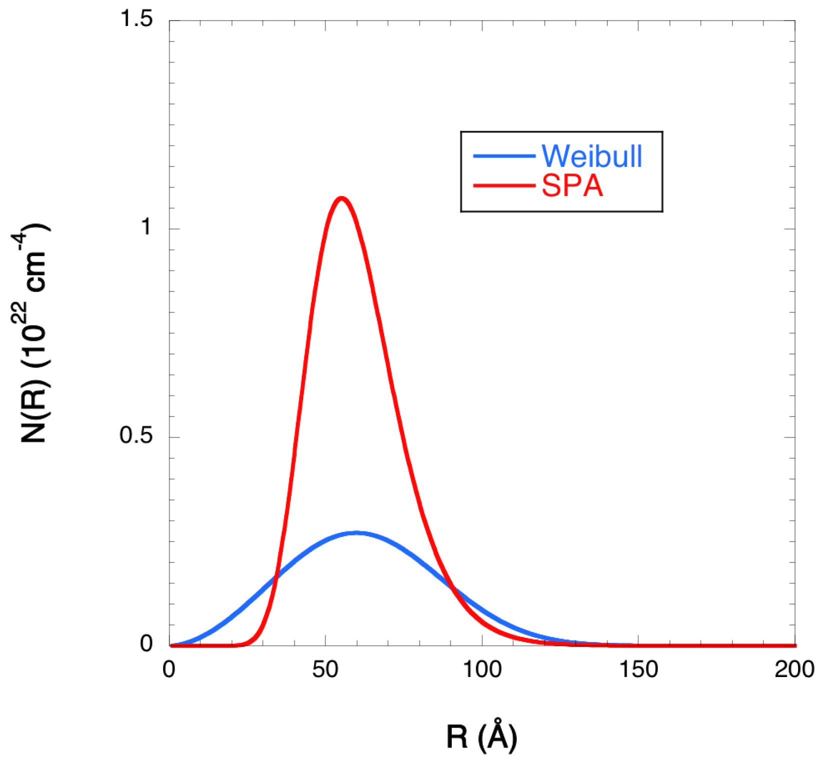
The SPA with user-defined functions and non-linear fits was applied here to the same data, and the results are shown in Figure 9a, where in Figure 9b, the SCSs are shown with the fit using the traditional fitting procedure with a Weibull SDF, taking into account corrections for the wavelength spread ( = 18%) and for multiple scattering. The Weibull SDF obtained with the fitting procedure and the lognormal SDF calculated with the SPA are compared in Figure 10.
The Ludox HS30 average radius and the volume fraction were found to be 61.3 ± 19.0 Å and 0.41 ± 0.13% with the SPA and 62.3 ± 2.3 Å and 0.25 ± 0.01% with the fitting procedure, respectively. The values and the SDFs obtained by the SPA and by the fitting procedure are in surprisingly good agreement with each other, bearing in mind the differences in the two procedures. The estimated uncertainties in the case of the SPA are larger, but still acceptable, as this is largely justified by the simplicity of the SPA method.
7. Conclusions
The SPA was used to perform a simplified analysis of the SAS data of polydisperse samples using simple interpolations employing commercial software, and it does not require a high level of computational skills. To summarize, the SPA can be applied when the following conditions are met:
- •
- Two-phase system;
- •
- Isotropic scattering;
- •
- Sharp interfaces of the inhomogeneities;
- •
- The Q-range includes both the Guinier and Porod approximations;
- •
- Presence of one family of inhomogeneities, described by a lognormal SDF;
- •
- The presence formalism has been developed for spherical inhomogeneities; however, it can be extended to other shapes.
The SPA provides the log-normal SDF of the investigated samples by performing the interpolation of the two approximated trends at small and large Q values, where the three parameters needed to define the SDF are calculated numerically from the optimized parameters. The check-list below summarizes the workflow of the determination of the SDF once the experimental SCSs are available:
The SPA was applied to both simulated (with and without an additional incoherent background) and experimental SCSs, and in all cases, the validity of the proposed method was demonstrated, where the values of the physical quantities were clearly reproduced and their uncertainties were larger than those estimated with the traditional fitting method. Last but not least, in many large-scale facilities, the simple SPA approach can be applied to real-time analysis during experiments for the efficient tuning of experimental details.
Funding
This research received no external funding.
Institutional Review Board Statement
Not applicable.
Informed Consent Statement
Not applicable.
Acknowledgments
Roberto Caciuffo is warmely acknowledged for his critical reading of the manuscript.
Conflicts of Interest
The authors declare no conflict of interest.
Abbreviations
The following abbreviations are used in this manuscript:
| ED | electron density |
| RID | refraction index density |
| SAS | small-angle scattering |
| SCS | scattering cross-section |
| SDF | size distribution function |
| SLD | scattering length density |
| SPA | simplified polydispersion analysis |
References
- Kostorz, G. Treatise on Materials Science and Technology; Academic Press: New York, NY, USA, 1979; Volume 15, pp. 227–289. [Google Scholar]
- Eberbeck, D.; Bläsing, J. Investigation of particle size distribution and aggregate structure of various ferrofluids by small-angle scattering experiments. J. Appl. Crystallogr. 1999, 32, 273–280. [Google Scholar] [CrossRef] [Green Version]
- Asri Ani, S.; Darminto; Giri Rachman Putra, E. Particle Size Distribution Models of Small Angle Neutron Scattering Pattern on Ferrofluids. AIP Conf. Proc. 2010, 1202, 73–76. [Google Scholar]
- Staron, P.; Jamnig, B.; Leitner, H.; Ebner, R.; Clemens, H. Small-angle neutron scattering analysis of the precipitation behaviour in a maraging steel. J. Appl. Crystallogr. 2003, 36, 415–419. [Google Scholar] [CrossRef]
- Alinger, M.; Odette, G.; Hoelzer, D. On the role of alloy composition and processing parameters in nanocluster formation and dispersion strengthening in nanostuctured ferritic alloys. Acta Mater. 2009, 57, 392–406. [Google Scholar] [CrossRef]
- Perrard, F.; Deschamps, A.; Bley, F.; Donnadieu, P.; Maugis, P. A small-angle neutron scattering study of fine-scale NbC precipitation kinetics in the α-Fe–Nb–C system. J. Appl. Crystallogr. 2006, 39, 473–482. [Google Scholar] [CrossRef] [Green Version]
- Del Genovese, D.; Rösler, J.; Strunz, P.; Mukherji, D.; Gilles, R. Microstructural characterization of a modified 706-type Ni-Fe superalloy by small-angle neutron scattering and electron microscopy. Met. Mater. Trans. 2005, 35, 3439–3450. [Google Scholar] [CrossRef]
- Pauw, B.; Kästner, C.; Thünemann, A. Nanoparticle size distribution quantification: Results of a small-angle X-ray scattering inter-laboratory comparison. J. Appl. Crystallogr. 2017, 50, 1280–1288. [Google Scholar] [CrossRef] [Green Version]
- Glade, S.; Wirth, B.; Odette, G.; Asoka-Kumar, P.; Sterne, P.; Howell, R. Positron annihilation spectroscopy and small-angle neutron scattering characterization of the effect of Mn on the nanostructural features formed in irradiated Fe-Cu-Mn alloys. Philos. Mag. 2005, 85, 629–639. [Google Scholar] [CrossRef]
- Vogel, M.; Kraft, O.; Staron, P.; Clemens, H.; Rauh, R.; Arzt, E. Microstructure of die-cast alloys Mg-Zn-Al(-Ca): A study by electron microscopy and small-angle neutron scattering. Z. Für Met. 2003, 94, 564–571. [Google Scholar] [CrossRef]
- Wiskel, J.; Ivey, D.; Henein, H. The Effects of Finish Rolling Temperature and Cooling Interrupt Conditions on Precipitation in Microalloyed Steels Using Small Angle Neutron Scattering. Met. Mater. Trans. 2008, 39, 116–124. [Google Scholar] [CrossRef]
- Krauthäuser, H.; Heitmann, W.K.A.; Nimtz, G. Small-Angle X-ray Scattering Analysis of Particle-Size Distributions of Mesoscopic Metallic Systems with Consideration of the Particle Form Factor. J. Appl. Crystallogr. 1994, 27, 558–562. [Google Scholar] [CrossRef]
- Mori, Y.; Furukawa, M.; Hayashi, T.; Nakamura, K. Size Distribution of Gold Nanoparticles Used by Small Angle X-ray Scattering. Part. Sci. Technol. 2006, 24, 97–103. [Google Scholar] [CrossRef]
- Marlaud, T.; Deschamps, A.; Bley, F.; Lefebvre, W.; Baroux, B. Evolution of precipitate microstructures during the retrogression and re-ageing heat treatment of an Al-Zn-Mg-Cu alloy. Acta Mater. 2010, 58, 4814–4826. [Google Scholar] [CrossRef]
- Agbabiaka, A.; Wiltfong, M.; Park, C. Small Angle X-ray Scattering Technique for the Particle Size Distribution of Nonporous Nanoparticles. J. Nanopart. 2013, 2013, 73–76. [Google Scholar] [CrossRef]
- Neilson, G. Small-angle X-ray scattering analysis of particle size distributions of colloidal Th2O sol. J. Appl. Crystallogr. 1973, 6, 386–392. [Google Scholar] [CrossRef]
- Bauer, P.; Amenitsch, H.; Baumgartner, B.; Köberl, G.; Rentenberger, C.; Winkler, P. In-situ aerosol nanoparticle characterization by small angle X-ray scattering at ultra-low volume fraction. Nat. Commun. 2019, 10, 1122. [Google Scholar] [CrossRef] [Green Version]
- Huige, D.; Zhixiang, W.; Dengxin, H. Precise size distribution measurement of aerosol particles and fog droplets in the open atmosphere. Opt. Express 2019, 27, A890–A908. [Google Scholar]
- Berg Rasmussen, F.; Molenbroek, A.M.C.B.; Feidenhans, R. Particle Size Distribution of an Ni/SiO2 Catalyst Determined by ASAXS. J. Catal. 2000, 190, 205–208. [Google Scholar] [CrossRef]
- Ma, S.; Deng, J.; Xu, Y.; Tao, W.; Wang, X.; Lin, Z.; Zhong, W. Pollen-like self-supported 327 FeIr alloy for improved hydrogen evolution reaction in acid electrolyte. J. Energy Chem. 2022, 66, 560–565. [Google Scholar] [CrossRef]
- Shen, S.; Hu, Z.; Zhang, H.; Song, K.; Wang, Z.; Lin, Z.; Zhang, Q.; Gu, L.; Zhong, W. Highly Active Si Sites Enabled by Negative 329 Valent Ru for Electrocatalytic Hydrogen Evolution in LaRuSi. Angew. Chem. Int. Ed. 2022, 61, e202206460. [Google Scholar] [CrossRef]
- Beaucage, G.; Kammlerb, H.; Pratsinis, S. Particle Size Distributions from Small-Angle Scattering Using Global Scattering Functions. J. Appl. Crystallogr. 2004, 37, 523–535. [Google Scholar] [CrossRef]
- Breßler, I.; Kohlbrecher, J.; Thünemann, A. SASfit: A tool for small-angle scattering data analysis using a library of analytical expressions. J. Appl. Crystallogr. 2015, 48, 1587–1598. [Google Scholar] [CrossRef] [PubMed]
- Carsughi, F.; Giacometti, A.; Gazzillo, D. Small-angle scattering data analysis for dense polydisperse systems: The FLAC program. Comput. Phys. Commun. 2000, 133, 66–75. [Google Scholar] [CrossRef] [Green Version]
- Ilavsky, J.; Jemian, P. Irena: Tool Suite Modelling Analysis Small-Angle Scatt. J. Appl. Crystallogr. 2009, 42, 347–353. [Google Scholar] [CrossRef]
- Jeffries, C.M.; Ilavsky, J.; Martel, A.; Hinrichs, S.; Meyer, A.; Pedersen, J.; Sokolova, A.; Svergun, D. Small-angle X-ray and neutron scattering. Nat. Rev. Methods Prim. 2021, 1, 70. [Google Scholar] [CrossRef]
- Guinier, A.; Fournet, A. Small-Angle Scattering of X-rays; Wiley: New York, NY, USA, 1955. [Google Scholar]
- Glatter, O.; Kratky, O. Small-Angle X-ray Scattering; Academic Press: London, UK, 1982. [Google Scholar]
- Carsughi, F.; Schwahn, D. Small-angle neutron scattering from silica particles in solution with different concentrations. Phys. B Condens. Matter 1997, 234–236, 343–346. [Google Scholar] [CrossRef]
Figure 1.
SDFs used to simulate the SCSs of polydisperse inhomogeneities; are normalized to ensure a volume fraction of 1%; = 20 Å; four values of are considered (0.1, 0.2, 0.3, and 0.4).
Figure 1.
SDFs used to simulate the SCSs of polydisperse inhomogeneities; are normalized to ensure a volume fraction of 1%; = 20 Å; four values of are considered (0.1, 0.2, 0.3, and 0.4).

Figure 2.
Simulated SCSs of a lognormal SDF of spherical inhomogeneities; are normalized to ensure a volume fraction of 1%; = 20 Å; four values of are considered (0.1, 0.2, 0.3, and 0.4). The Guinier and the Porod approximations are present in the investigated Q range.
Figure 2.
Simulated SCSs of a lognormal SDF of spherical inhomogeneities; are normalized to ensure a volume fraction of 1%; = 20 Å; four values of are considered (0.1, 0.2, 0.3, and 0.4). The Guinier and the Porod approximations are present in the investigated Q range.

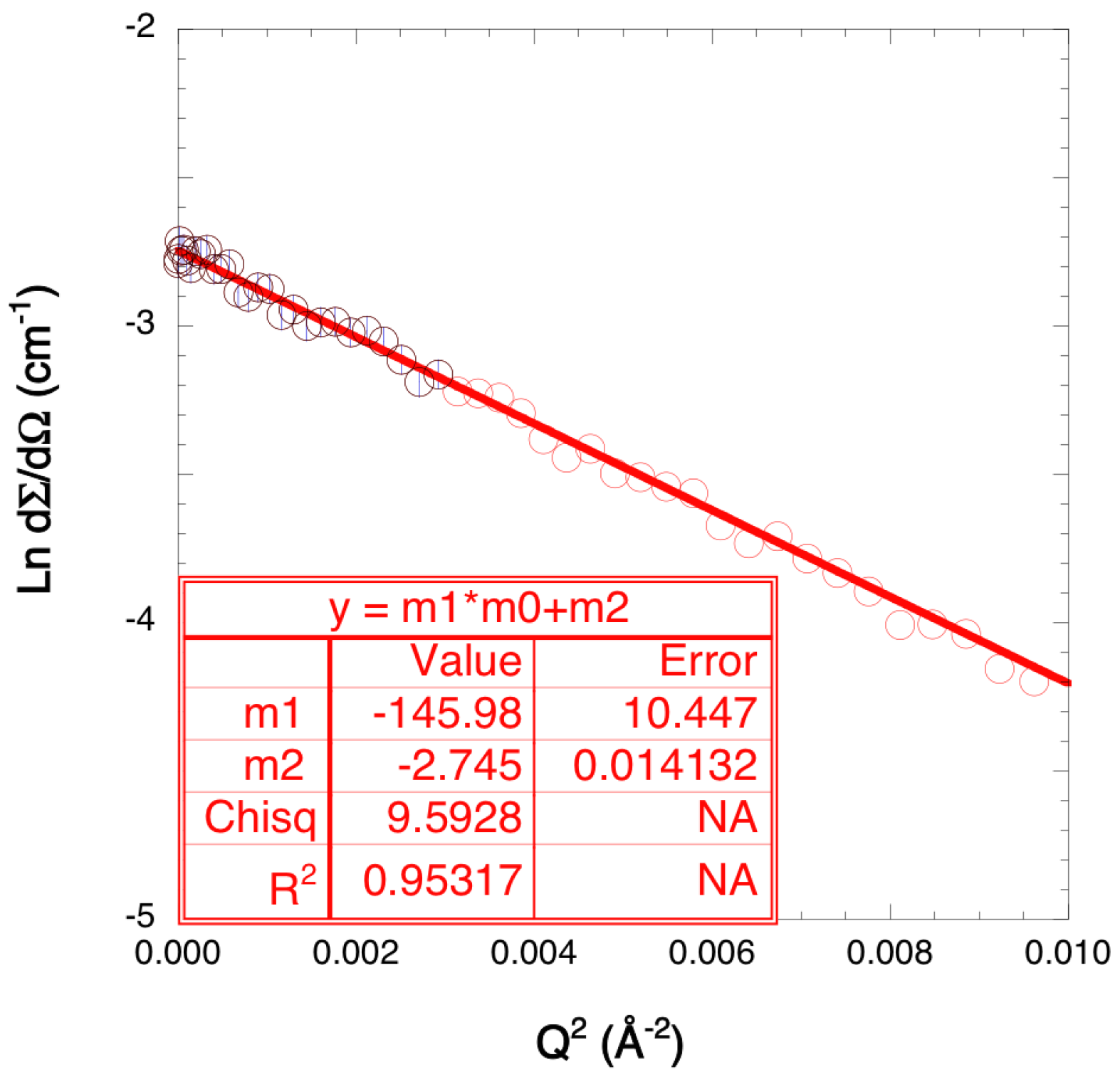
Figure 3.
Guinier approximation of the simulated SCS by using the SDF with = 0.2. The points used for the Guinier approximation are shown with black symbols, while the others are red. The fit is shown with a red line.
Figure 3.
Guinier approximation of the simulated SCS by using the SDF with = 0.2. The points used for the Guinier approximation are shown with black symbols, while the others are red. The fit is shown with a red line.

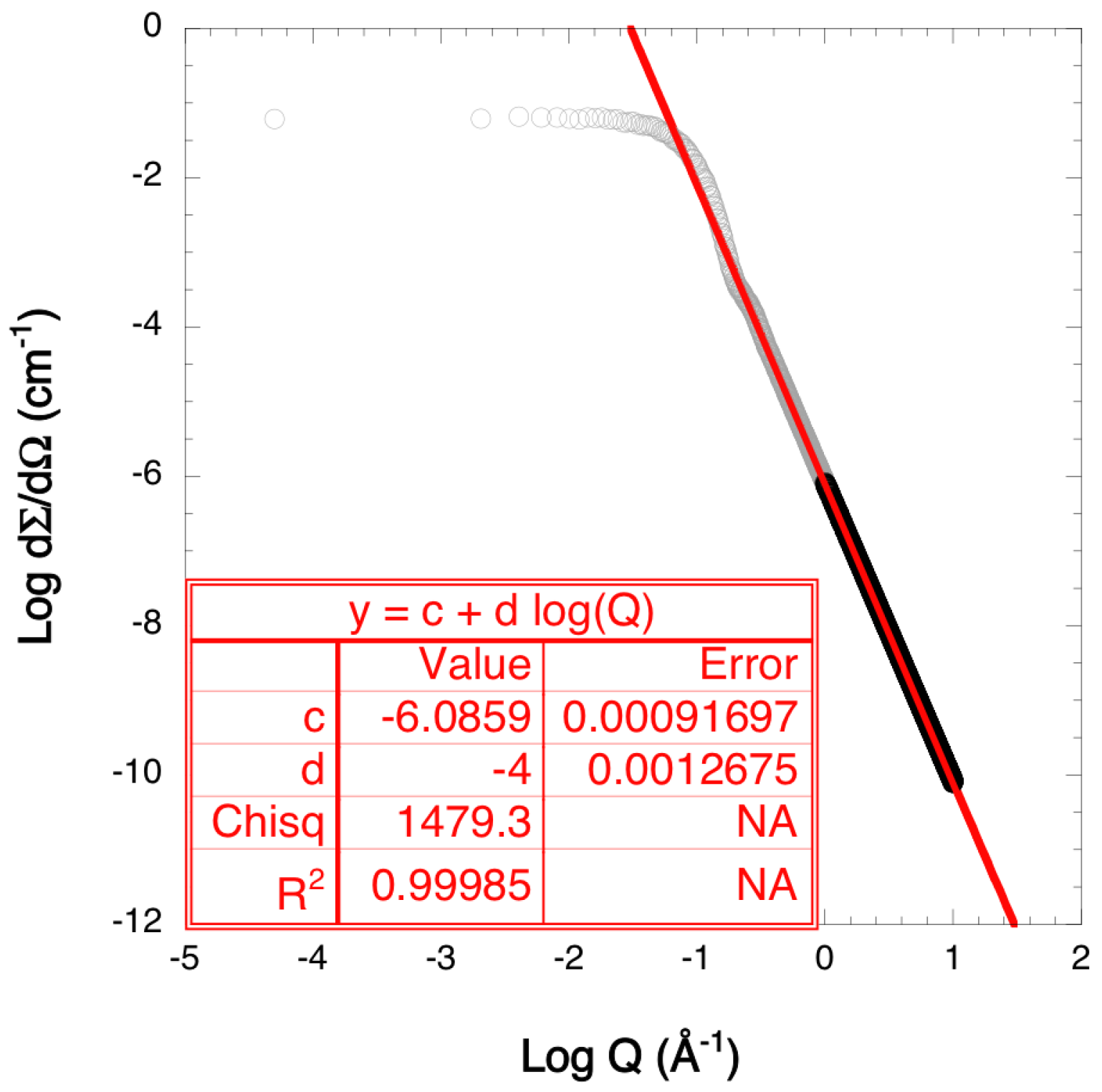
Figure 4.
Porod approximation of the simulated SCS by using the SDF with = 0.2. The points used for the fit are shown with black symbols, while the others are red. The fit is shown with a red line.
Figure 4.
Porod approximation of the simulated SCS by using the SDF with = 0.2. The points used for the fit are shown with black symbols, while the others are red. The fit is shown with a red line.

Figure 5.
SDFs reconstructed with the parameters (, and ) calculated with the SPA for the four cases ( = 0.1, 0.2, 0.3 and 0.4). The original SDFs are shown in Figure 1.
Figure 5.
SDFs reconstructed with the parameters (, and ) calculated with the SPA for the four cases ( = 0.1, 0.2, 0.3 and 0.4). The original SDFs are shown in Figure 1.

Figure 6.
Guinier approximation of the simulated SCS by using the SDF with = 0.4 and an incoherent background of 1.0 × 10 cm. The points used for the Guinier approximation are shown with black symbols, while the others are red. The fit is shown with a red line.
Figure 6.
Guinier approximation of the simulated SCS by using the SDF with = 0.4 and an incoherent background of 1.0 × 10 cm. The points used for the Guinier approximation are shown with black symbols, while the others are red. The fit is shown with a red line.

Figure 7.
Porod approximation of the simulated SCS by using the SDF with = 0.4 and an incoherent background of 1.0 × 10 cm. The points used are shown with black symbols, while the others are red. The fit is shown with a red line.
Figure 7.
Porod approximation of the simulated SCS by using the SDF with = 0.4 and an incoherent background of 1.0 × 10 cm. The points used are shown with black symbols, while the others are red. The fit is shown with a red line.

Figure 8.
SDFs reconstructed with the parameters (, , and ) calculated with the SPA for the case without (red line) and with additional backgrounds of 1.0 × 10 (B1—blue line), 1.0 × 10 (B2—green line), and 1.0 × 10 cm (B3—yellow line). The original SDF is also shown for comparison (black line).
Figure 8.
SDFs reconstructed with the parameters (, , and ) calculated with the SPA for the case without (red line) and with additional backgrounds of 1.0 × 10 (B1—blue line), 1.0 × 10 (B2—green line), and 1.0 × 10 cm (B3—yellow line). The original SDF is also shown for comparison (black line).

Figure 9.
Analysis of experimental SCS of Ludox silica particles HS30 with a 0.3% volume fraction: (a) The SPA with the fits of the Guinier (red line), as well as of the Porod (blue line) approximations along with the values of the optimized parameters and their uncertainties. The points used for both fits are shown with black symbols, while the others are red. (b) A fitting procedure with a Weibull SDF, where corrections for the wavelength spread ( = 18%) and for the multiple scattering were applied [29].

Figure 10.
Ludox silica particles HS30 with a 0.3% volume fraction: the Weibull SDF (blue line) obtained with the fitting procedure, with corrections for the wavelength spread ( = 18%) and for the multiple scattering, and the lognormal SDF (red line) calculated with the SPA.
Figure 10.
Ludox silica particles HS30 with a 0.3% volume fraction: the Weibull SDF (blue line) obtained with the fitting procedure, with corrections for the wavelength spread ( = 18%) and for the multiple scattering, and the lognormal SDF (red line) calculated with the SPA.


Table 1.
Nominal and calculated values of the three parameters of the lognormal SDF of spherical inhomogeneities obtained by applying the SPA to the simulated SCSs.
Table 1.
Nominal and calculated values of the three parameters of the lognormal SDF of spherical inhomogeneities obtained by applying the SPA to the simulated SCSs.
| Parameter | ||||
|---|---|---|---|---|
| nominal values | ||||
| ( cm) | ||||
| (Å) | ||||
| calculated values | ||||
| ( cm) | ||||
| (Å) | ||||
Table 2.
Nominal and calculated values of the main physical quantities, the number density N, the average radius , the average surface , and the volume fraction , of spherical inhomogeneities obtained by applyingthe SPA on the simulated SCS.
Table 2.
Nominal and calculated values of the main physical quantities, the number density N, the average radius , the average surface , and the volume fraction , of spherical inhomogeneities obtained by applyingthe SPA on the simulated SCS.
| Parameter | ||||
|---|---|---|---|---|
| nominal values | ||||
| N ( cm) | ||||
| (Å) | ||||
| ( cm | ||||
| calculated values | ||||
| N ( cm) | ||||
| (Å) | ||||
| ( cm | ||||
Table 3.
Calculated values of the three parameters of the lognormal SDF of spherical inhomogeneities obtained by the SPA of the simulated SCS with the backgrounds added to the case of = 0.4.
Table 3.
Calculated values of the three parameters of the lognormal SDF of spherical inhomogeneities obtained by the SPA of the simulated SCS with the backgrounds added to the case of = 0.4.
| Background (cm) | |||
|---|---|---|---|
| 1.0 × 10 | 1.0 × 10 | 1.0 × 10 | |
| calculated values | |||
| ( cm) | |||
| (Å) | |||
Publisher’s Note: MDPI stays neutral with regard to jurisdictional claims in published maps and institutional affiliations. |
© 2022 by the author. Licensee MDPI, Basel, Switzerland. This article is an open access article distributed under the terms and conditions of the Creative Commons Attribution (CC BY) license (https://creativecommons.org/licenses/by/4.0/).
Share and Cite
MDPI and ACS Style
Carsughi, F. Simplified Polydispersion Analysis of Small-Angle Scattering Data. Appl. Sci. 2022, 12, 10677. https://doi.org/10.3390/app122010677
AMA Style
Carsughi F. Simplified Polydispersion Analysis of Small-Angle Scattering Data. Applied Sciences. 2022; 12(20):10677. https://doi.org/10.3390/app122010677
Chicago/Turabian StyleCarsughi, Flavio. 2022. "Simplified Polydispersion Analysis of Small-Angle Scattering Data" Applied Sciences 12, no. 20: 10677. https://doi.org/10.3390/app122010677
Note that from the first issue of 2016, this journal uses article numbers instead of page numbers. See further details here.