
Centrifugal Test Replicated Numerical Model Updating for 3D Strutted Deep Excavation with the Response-Surface Method
 , ,
, ,
Abstract
:1. Introduction
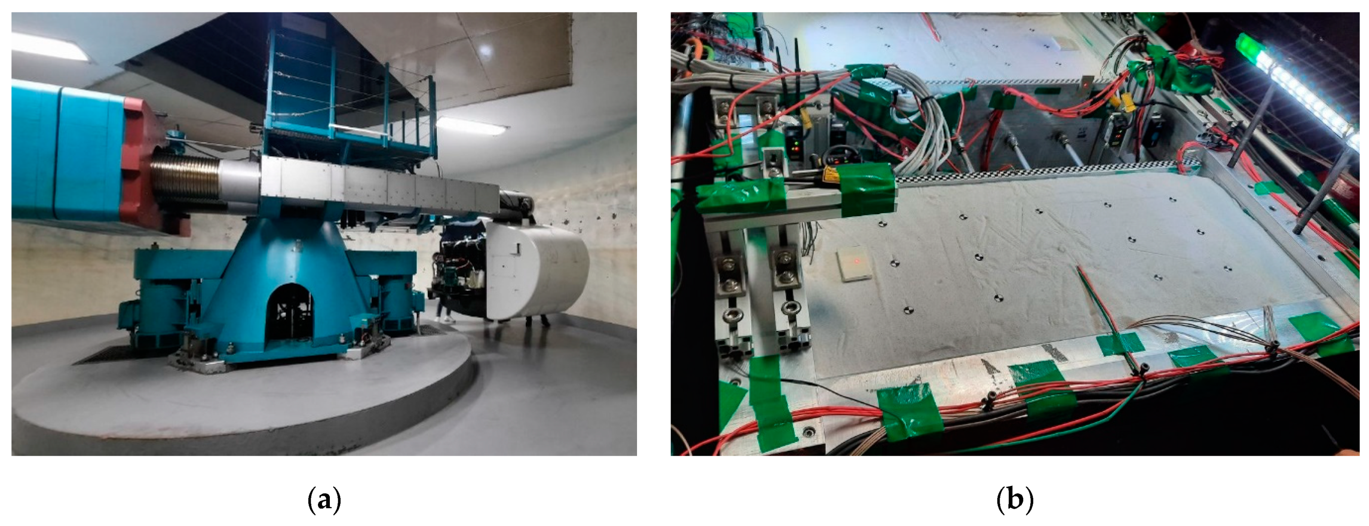
2. Centrifugal Test
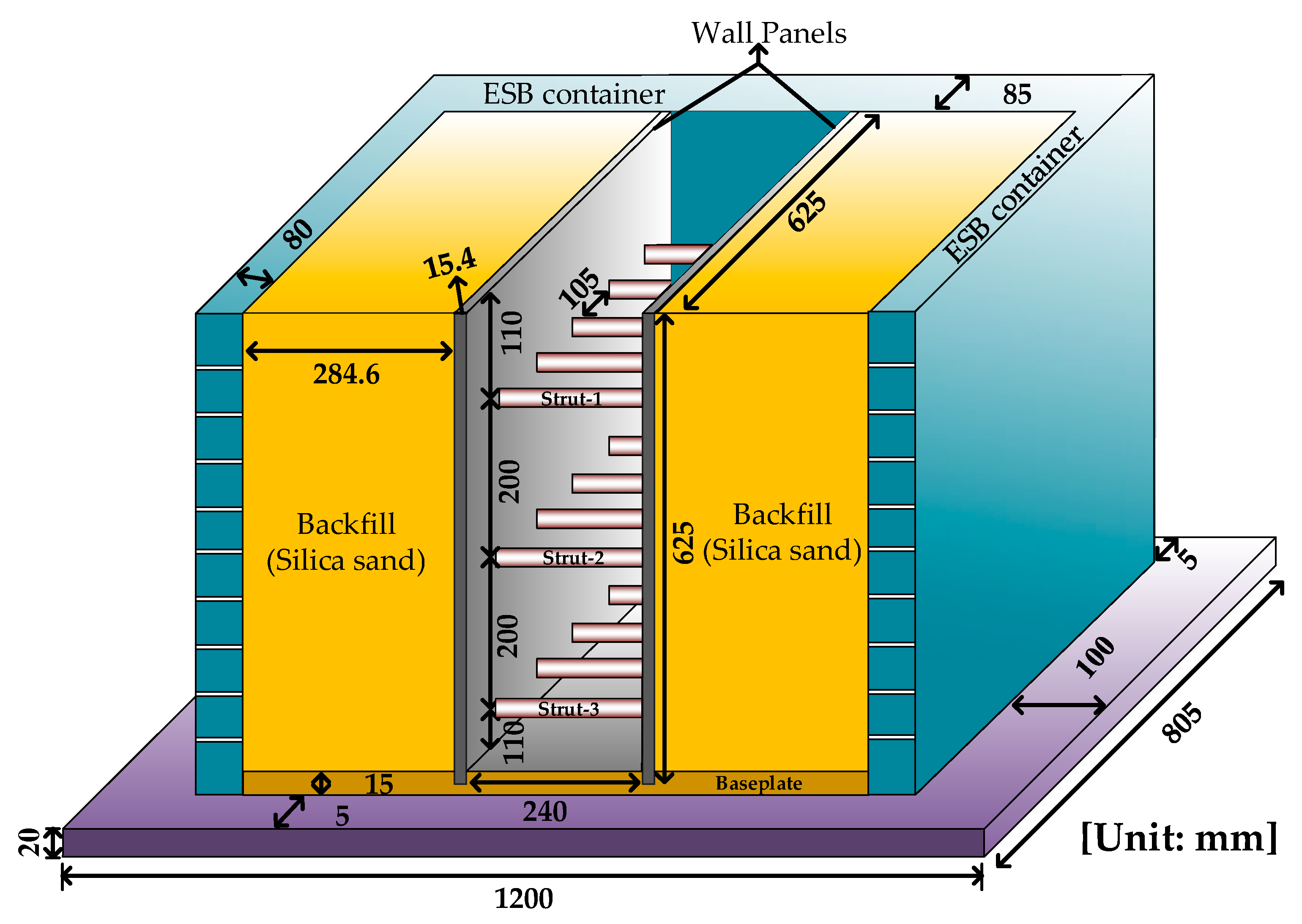
2.1. Test Model
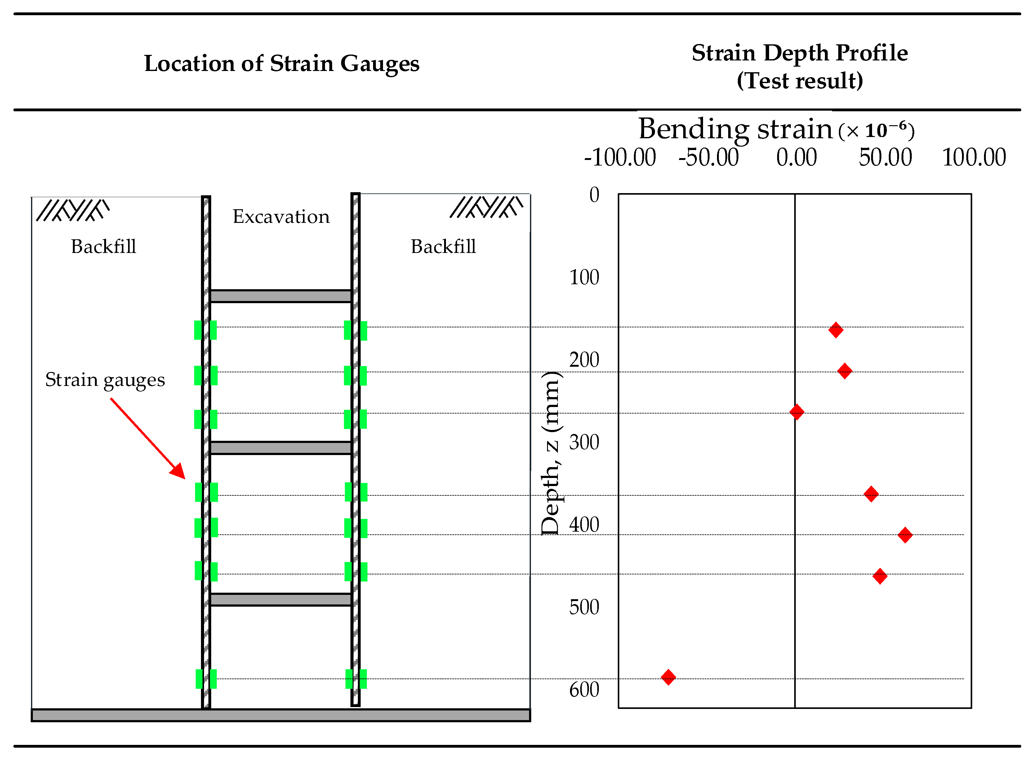
2.2. Test Result
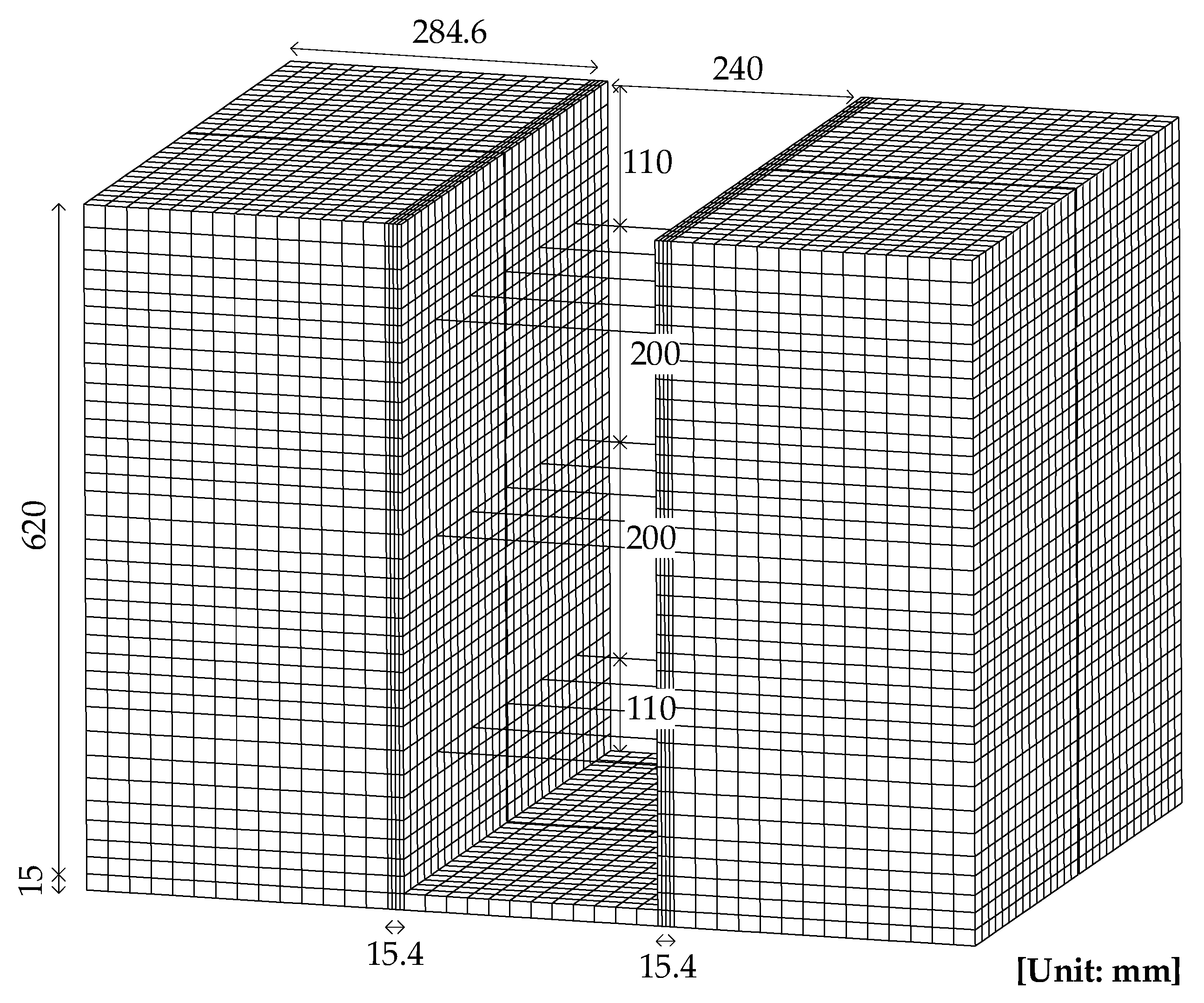
3. Numerical Model
3.1. Soil and Structure
3.2. Materials
4. Soil Parameter Updating
4.1. Response-Surface Method
4.2. Response-Surface Model
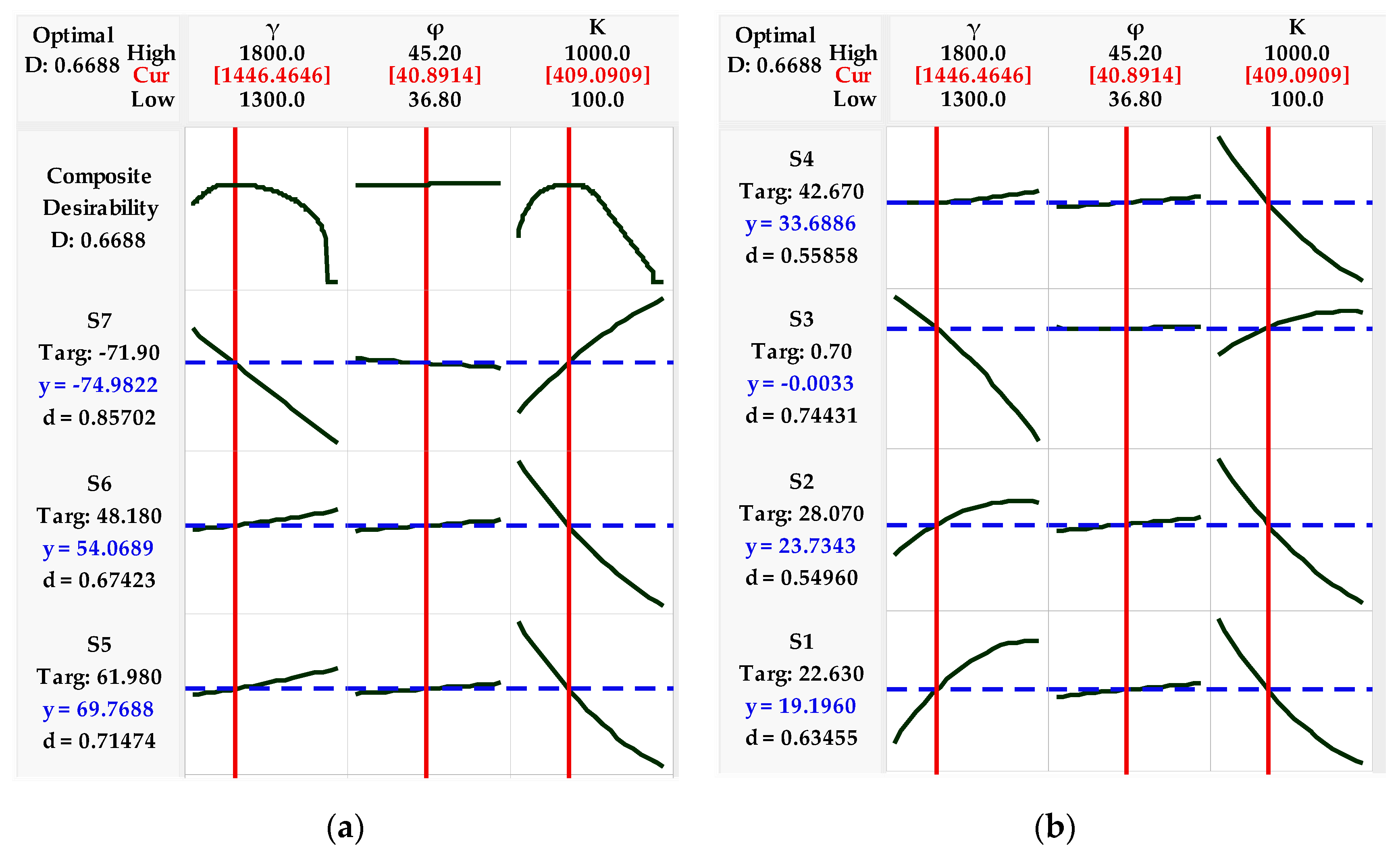
4.3. Updated Properties
5. Numerical Model Update and Validation
6. Conclusions
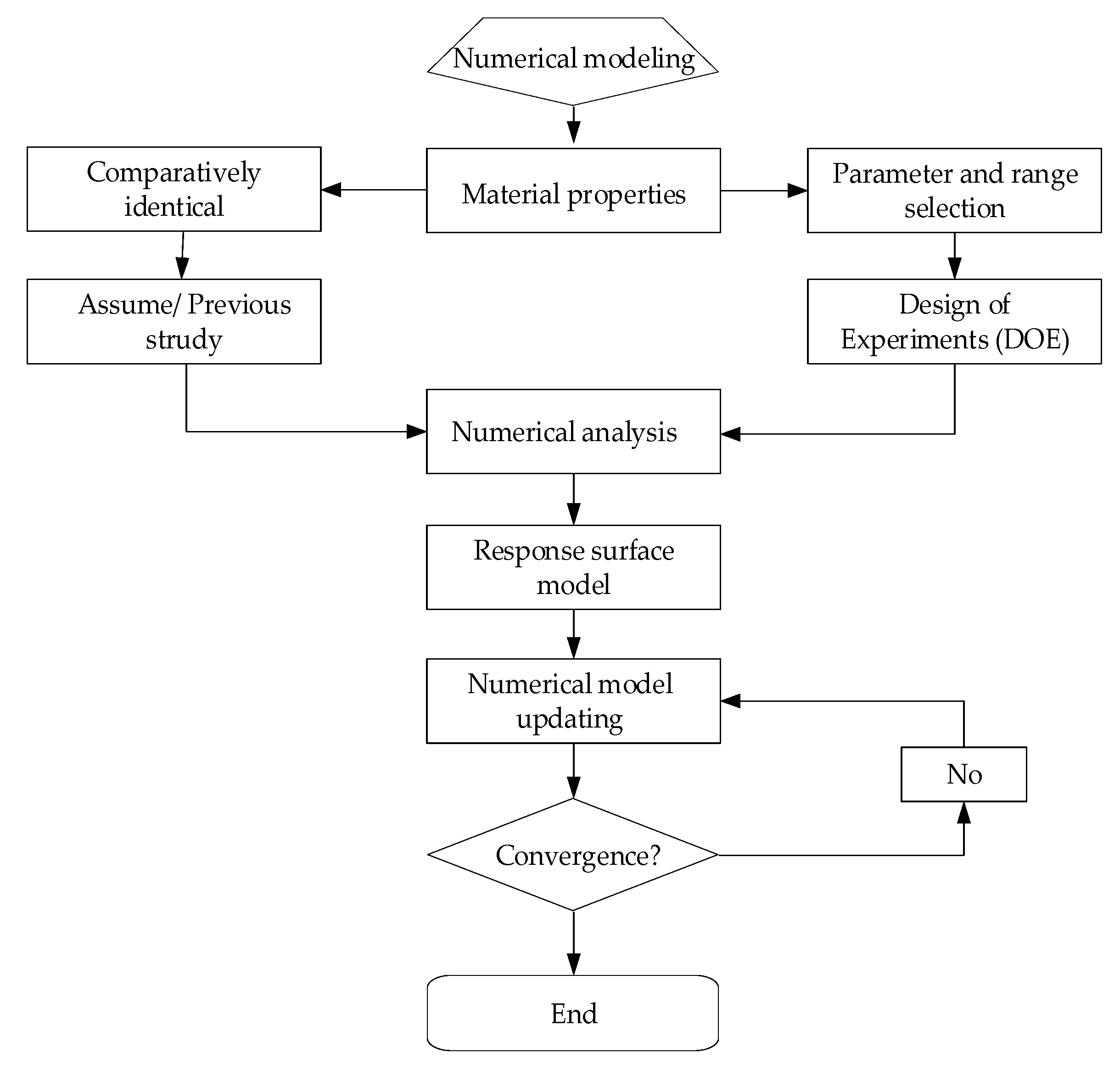
- Comparatively identical properties for particular types of soil were assumed. Suitable ranges for key parameters were selected. The design of experiments (DOE) was created. The structural responses were chosen. Numerical responses were obtained for each DOE. The response-surface (RS) model was created using those responses and DOE. Centrifugal responses were adopted in the RS model as a target, and updated soil parameters were obtained. The numerical model was updated by adopting the obtained parameters.
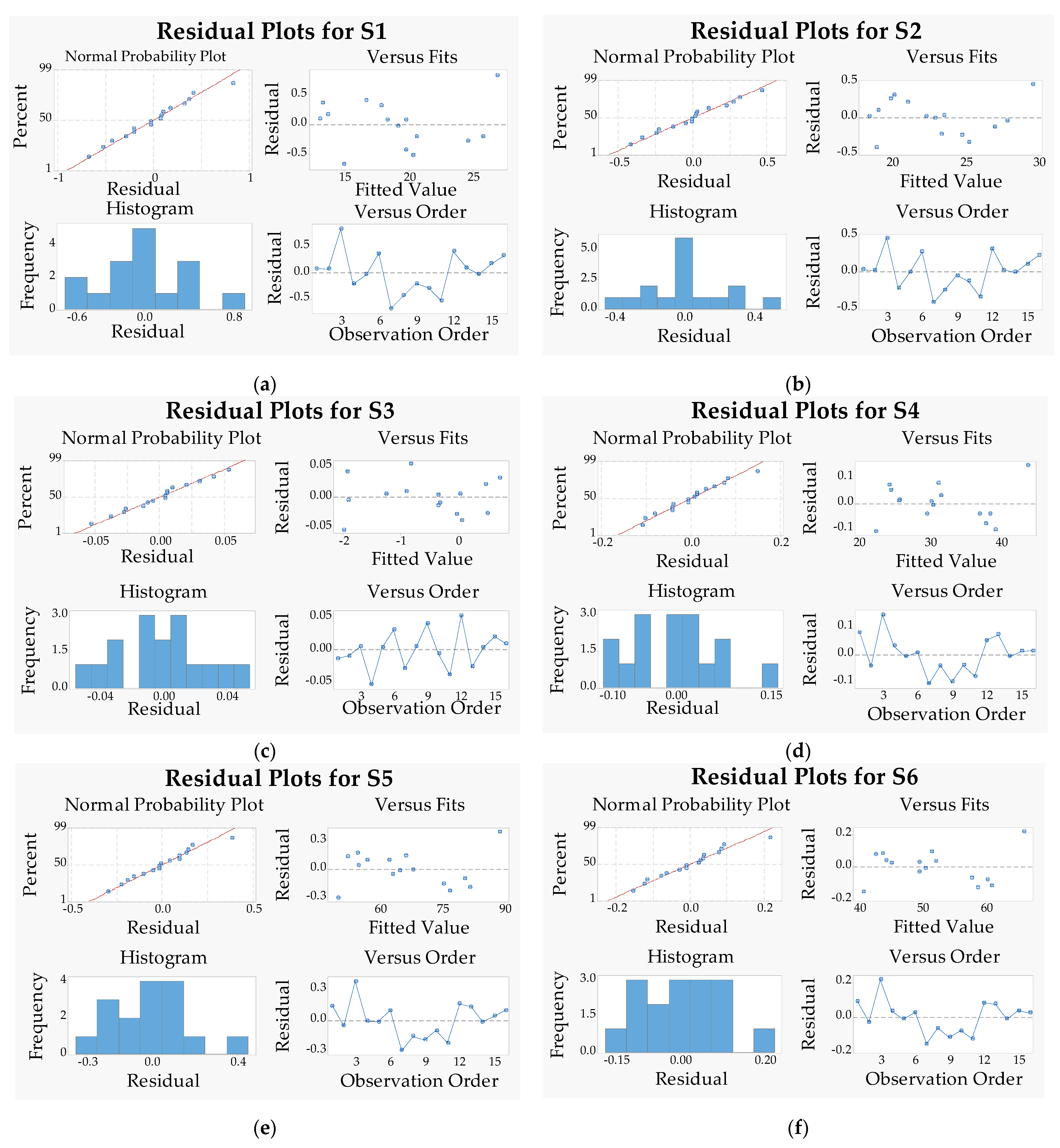
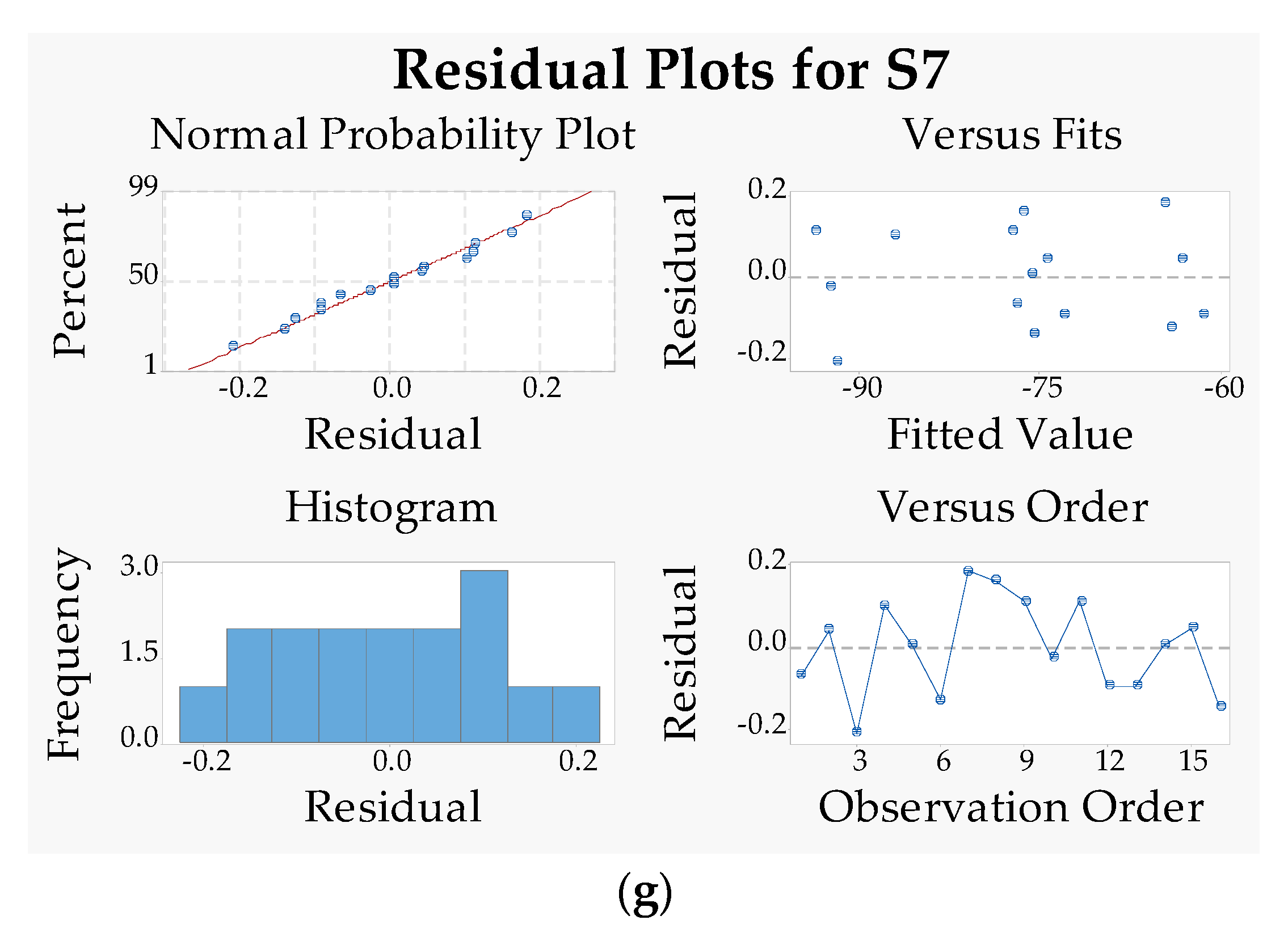
- The fitness and significance of the RS model were checked with the coefficient of determination ( and probability values for the obtained results (p-value).
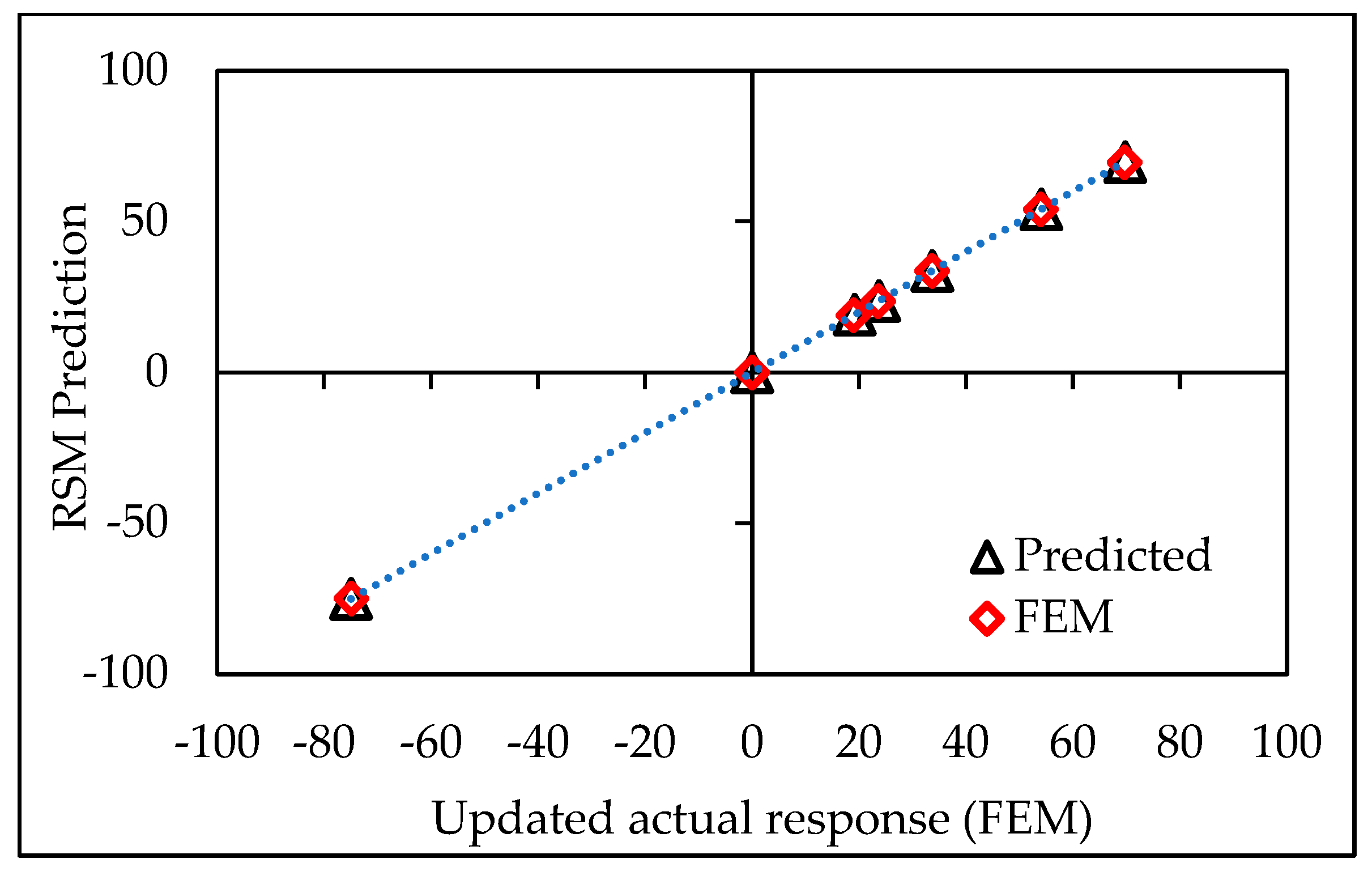
- Predictions from the RS model showed good consistency with the numerical model responses; the difference between these two was less than 0.5%.
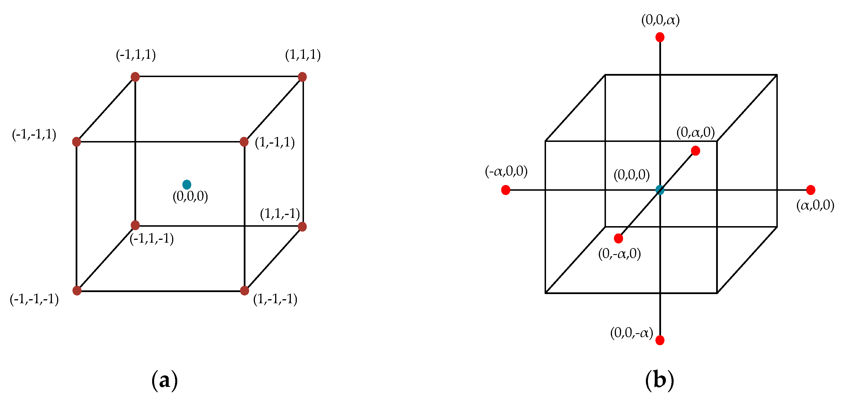
- The bending strain response of the small-scale numerical model and DOE of the central composite design could establish a well-fitted RS model. This analysis achieved the coefficient of determination ( by more than 95%.
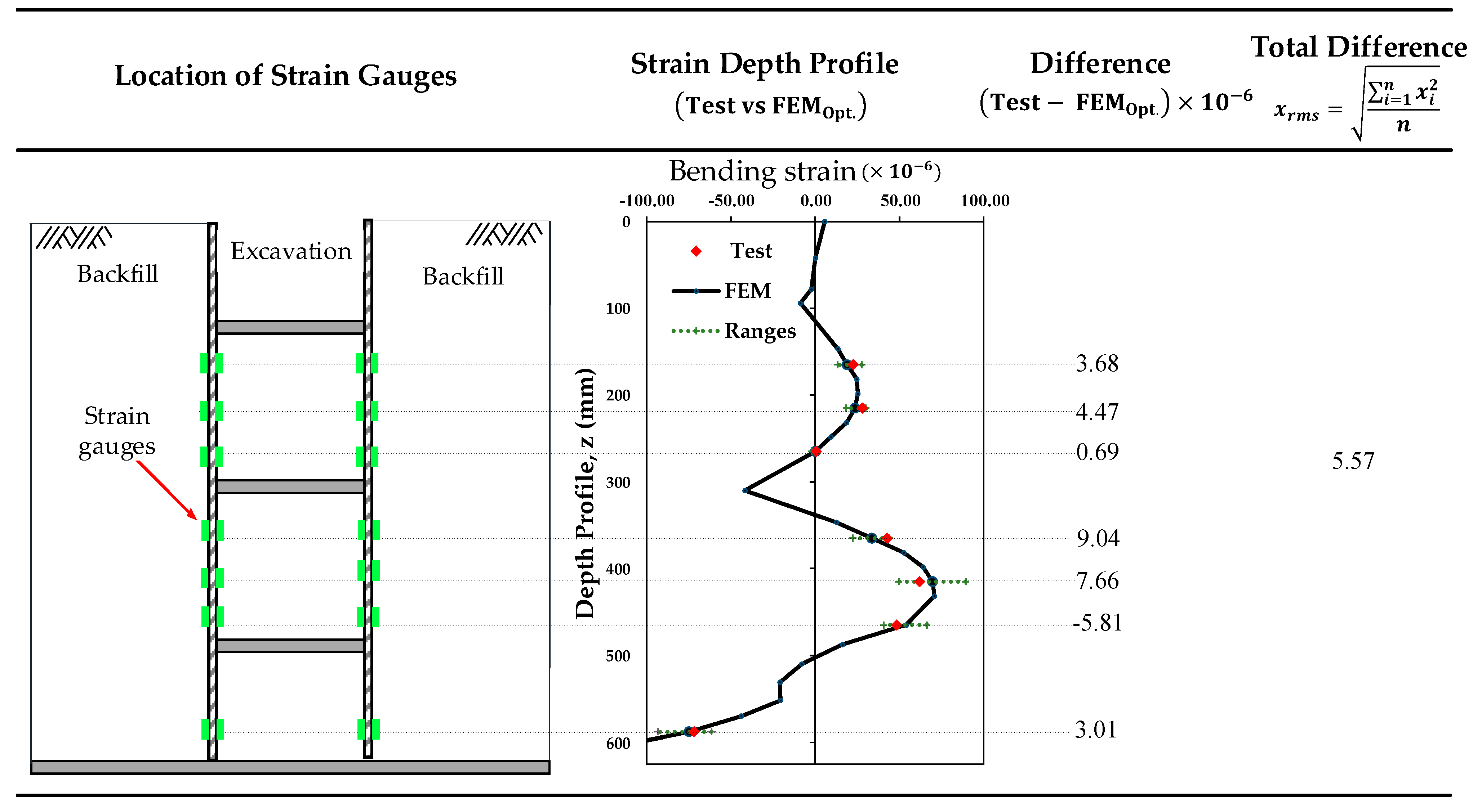
- Minimal differences between the test results and the numerical model were achieved.
- The ranges of the responses could be visualized for the particular ranges of soil properties.
- The updated numerical model showed reasonable agreement with the centrifugal test and it can be used for parametric analysis.
Author Contributions
Funding
Institutional Review Board Statement
Informed Consent Statement
Data Availability Statement
Acknowledgments
Conflicts of Interest
References
- Meng, F.-Y.; Chen, R.-P.; Wu, H.-N.; Xie, S.-W.; Liu, Y. Observed behaviors of a long and deep excavation and collinear underlying tunnels in Shenzhen granite residual soil. Tunn. Undergr. Space Technol. 2020, 103, 103504. [Google Scholar] [CrossRef]
- Yoo, C.; Lee, D. Deep excavation-induced ground surface movement characteristics—A numerical investigation. Comput. Geotech. 2008, 35, 231–252. [Google Scholar] [CrossRef]
- Ou, C.-Y.; Chiou, D.-C.; Wu, T.-S. Three-Dimensional Finite Element Analysis of Deep Excavations. J. Geotech. Eng. 1996, 122, 337–345. [Google Scholar] [CrossRef]
- Bose, S.K.; Som, N.N. Parametric study of a braced cut by finite element method. Comput. Geotech. 1998, 22, 91–107. [Google Scholar] [CrossRef]
- Karlsrud, K.; Andresen, L. Loads on Braced Excavations in Soft Clay. Int. J. Geomech. 2005, 5, 107–113. [Google Scholar] [CrossRef]
- Schäfer, R.; Triantafyllidis, T. The influence of the construction process on the deformation behaviour of diaphragm walls in soft clayey ground. Int. J. Numer. Anal. Methods Geomech. 2006, 30, 563–576. [Google Scholar] [CrossRef]
- Costa, P.A.; Borges, J.L.; Fernandes, M.M. Analysis of A Braced Excavation In Soft Soils Considering The Consolidation Effect. Geotech. Geol. Eng. 2007, 25, 617–629. [Google Scholar] [CrossRef]
- Finno, R.J.; Blackburn, J.T.; Roboski, J.F. Three-Dimensional Effects for Supported Excavations in Clay. J. Geotech. Geoenvironmental Eng. 2007, 133, 30–36. [Google Scholar] [CrossRef] [Green Version]
- Harahap, S.E.; Ou, C.-Y. Finite element analysis of time-dependent behavior in deep excavations. Comput. Geotech. 2020, 119, 103300. [Google Scholar] [CrossRef]
- Bahrami, M.; Khodakarami, M.I.; Haddad, A. 3D numerical investigation of the effect of wall penetration depth on excavations behavior in sand. Comput. Geotech. 2018, 98, 82–92. [Google Scholar] [CrossRef]
- Sankar, S.; Deb, C.K.; Sengupta, A. Estimation of Design Parameters for Braced Excavation: Numerical Study. Int. J. Geomech. 2013, 13, 234–247. [Google Scholar]
- ASHOUR, S.; Ünsever, Y.S. STATIC ANALYSES OF THE EFFECT OF DEEP EXCAVATION ON THE BEHAVIOUR OF AN ADJACENT PILE IN SAND. Uludağ Üniversitesi Mühendislik Fakültesi Derg. 2022, 27, 627–646. [Google Scholar] [CrossRef]
- Ng, C.W.W.; Shi, J.; Hong, Y. Three-dimensional centrifuge modelling of basement excavation effects on an existing tunnel in dry sand. Can. Geotech. J. 2013, 50, 874–888. [Google Scholar] [CrossRef]
- Meng, F.-y.; Chen, R.-p.; Xu, Y.; Wu, K.; Wu, H.-n.; Liu, Y. Contributions to responses of existing tunnel subjected to nearby excavation: A review. Tunn. Undergr. Space Technol. 2022, 119, 104195. [Google Scholar] [CrossRef]
- Finno, R.J.; Calvello, M. Supported Excavations: Observational Method and Inverse Modeling. J. Geotech. Geoenvironmental Eng. 2005, 131, 826–836. [Google Scholar] [CrossRef]
- Tang, Y.-G.; Kung, G.T.-C. Application of nonlinear optimization technique to back analyses of deep excavation. Comput. Geotech. 2009, 36, 276–290. [Google Scholar] [CrossRef]
- Rechea, C.; Levasseur, S.; Finno, R. Inverse analysis techniques for parameter identification in simulation of excavation support systems. Comput. Geotech. 2008, 35, 331–345. [Google Scholar] [CrossRef]
- Levasseur, S.; Malécot, Y.; Boulon, M.; Flavigny, E. Soil parameter identification using a genetic algorithm. Int. J. Numer. Anal. Meth. Geomech 2008, 32, 189–213. [Google Scholar] [CrossRef]
- Zhao, B.; Zhang, L.; Jeng, D.; Wang, J.; Chen, J. Inverse analysis of deep excavation using differential evolution algorithm. Int. J. Numer. Anal. Methods Geomech. 2015, 39, 115–134. [Google Scholar] [CrossRef]
- Hashash, Y.M.A.; Levasseur, S.; Osouli, A.; Finno, R.; Malecot, Y. Comparison of two inverse analysis techniques for learning deep excavation response. Comput. Geotech. 2010, 37, 323–333. [Google Scholar] [CrossRef]
- Wang, L.; Luo, Z.; Xiao, J.; Juang, C.H. Probabilistic Inverse Analysis of Excavation-Induced Wall and Ground Responses for Assessing Damage Potential of Adjacent Buildings. Geotech. Geol. Eng. 2014, 32, 273–285. [Google Scholar] [CrossRef]
- Juang, C.H.; Luo, Z.; Atamturktur, S.; Huang, H. Bayesian updating of soil parameters for braced excavations using field observations. J. Geotech. Geoenvironmental Eng. 2013, 139, 395–406. [Google Scholar] [CrossRef] [Green Version]
- Qi, X.-H.; Zhou, W.-H. An efficient probabilistic back-analysis method for braced excavations using wall deflection data at multiple points. Comput. Geotech. 2017, 85, 186–198. [Google Scholar] [CrossRef]
- Huang, Z.H.; Zhang, L.L.; Cheng, S.Y.; Zhang, J.; Xia, X.H. Back-Analysis and Parameter Identification for Deep Excavation Based on Pareto Multiobjective Optimization. J. Aerosp. Eng. 2015, 28, A4014007. [Google Scholar] [CrossRef]
- Ren, W.-X.; Chen, H.-B. Finite element model updating in structural dynamics by using the response surface method. Eng. Struct. 2010, 32, 2455–2465. [Google Scholar] [CrossRef]
- Kim, D.-S.; Kim, N.-R.; Choo, Y.W.; Cho, G.-C. A newly developed state-of-the-art geotechnical centrifuge in Korea. KSCE J. Civ. Eng. 2013, 17, 77–84. [Google Scholar] [CrossRef]
- Abaqus. Documentation, 2017; Dassault Systémes Simulia Corp.: Providence, RI, USA, 2017. [Google Scholar]
- Kim, D.-S.; Kim, N.-R.; Choo, Y.-W. Physical modeling of geotechnical systems using centrifuge. In Proceedings of the Korean Geotechical Society Conference, Incheon, Korea, 25–26 September 2009; Korean Geotechnical Society: Seoul, Korea, 2009. [Google Scholar]
- Grasso, S.; Lentini, V.; Sammito, M.S.V. A New Biaxial Laminar Shear Box for 1g Shaking Table Tests on Liquefiable Soils. In Proceedings of the 4th International Conference on Performance Based Design in Earthquake Geotechnical Engineering, Beijing, China, 15–17 July 2022; Springer International Publishing: Cham, Switzerland, 2022. [Google Scholar]
- Maurya, N.K.; Maurya, M.; Srivastava, A.K.; Dwivedi, S.P.; Kumar, A.; Chauhan, S. Investigation of mechanical properties of Al 6061/SiC composite prepared through stir casting technique. Mater. Today-Proc. 2020, 25, 755–758. [Google Scholar] [CrossRef]
- Kim, J.H.; Choo, Y.W.; Kim, D.J.; Kim, D.S. Miniature Cone Tip Resistance on Sand in a Centrifuge. J. Geotech. Geoenvironmental Eng. 2016, 142, 04015090. [Google Scholar] [CrossRef]
- Bolton, M.D. The strength and dilatancy of sands. Geotechnique 1986, 36, 65–78. [Google Scholar] [CrossRef] [Green Version]
- Khoiri, M.; Ou, C.-Y. Evaluation of deformation parameter for deep excavation in sand through case histories. Comput. Geotech. 2013, 47, 57–67. [Google Scholar] [CrossRef]
- Janbu, N. Soil compressibility as determined by oedometer and triaxial tests. In Proceedings of the European Conference on Soil Mechanics and Foundation Engineering, Wiesbaden, Germany, 15–18 October 1963; Norwegian Geotechnical Institute: Oslo, Norway, 1963. [Google Scholar]
- Duncan, J.M. Strength, Stress-Strain and Bulk Modulus Parameters for Finite Element Analyses of Stresses and Movements in Soil Masses; Report No: UCB/GT/80-01; University of California: California, CA, USA, 1980. [Google Scholar]
- Jaky, J. The coefficient of earth pressure at rest. J. Soc. Hung. Archit. Eng. 1944, 78, 355–358. [Google Scholar]
- Yousefi, M.; Safikhani, H.; Jabbari, E.; Yousefi, M.; Tahmsbi, V. Numerical modeling and Optimization of Respirational Emergency Drug Delivery Device using Computational Fluid Dynamics and Response Surface Method J International Journal of Engineering. Int. J. Eng. 2021, 34, 547–555. [Google Scholar] [CrossRef]
- Myers, R.H.; Montgomery, D.C.; Anderson-Cook, C.M. Response Surface Methodology: Process and Product Optimization Using Designed Experiments; John Wiley & Sons: Hoboken, NJ, USA, 2016; ISBN 1118916034. [Google Scholar]
- Box, G.E.P.; Wilson, K.B. On the Experimental Attainment of Optimum Conditions. Breakthr. Stat. 1951, 13, 1–38. [Google Scholar] [CrossRef]
- Hang, Y.; Qu, M.; Ukkusuri, S. Optimizing the design of a solar cooling system using central composite design techniques. Energy Build. 2011, 43, 988–994. [Google Scholar] [CrossRef]
- Rahman, M.M.; Nahar, T.T.; Kim, D.; Park, D.-W. Location Sensitivity of Non-structural Component for Channel-type Auxiliary Building Considering Primary-secondary Structure Interaction. Int. J. Eng. 2022, 35, 1268–1282. [Google Scholar] [CrossRef]
- Alin, A. Minitab. Wiley Interdiscip. Rev. Comput. Stat. 2010, 2, 723–727. [Google Scholar] [CrossRef]
- Sahu, N.K.; Andhare, A.B. Multiobjective optimization for improving machinability of Ti-6Al-4V using RSM and advanced algorithms. J. Comput. Des. Eng. 2018, 6, 1–12. [Google Scholar] [CrossRef]
- Baligidad, S.M.; Chandrasekhar, U.; Elangovan, K.; Shankar, S. RSM Optimization of Parameters influencing Mechanical properties in Selective Inhibition Sintering. Mater. Today Proc. 2018, 5, 4903–4910. [Google Scholar] [CrossRef]
- Joglekar, A.M.; May, A.; Graf, E.; Saguy, I. Product Excellence through Experimental Design. In Product Excellence through Experimental Design; Springer Science & Business Media: New York, NY, USA, 1991. [Google Scholar]
- Noordin, M.Y.; Venkatesh, V.C.; Sharif, S.; Elting, S.; Abdullah, A. Application of response surface methodology in describing the performance of coated carbide tools when turning AISI 1045 steel. J. Mater. Process. Technol. 2004, 145, 46–58. [Google Scholar] [CrossRef] [Green Version]
- Jo, S.-B.; Ha, J.-G.; Yoo, M.; Choo, Y.W.; Kim, D.-S. Seismic behavior of an inverted T-shape flexible retaining wall via dynamic centrifuge tests. Bull. Earthq. Eng. 2014, 12, 961–980. [Google Scholar] [CrossRef]
- Hoffman, P. Contributions of Janbu and Lade as applied to Reinforced Soil. In Proceedings of the 17th Nordic Geotechnical Meeting, Reykjavik, Iceland, 25–28 May 2016. [Google Scholar]


| Factor | Range | Cubic | Axial | Central | ||
|---|---|---|---|---|---|---|
| Min. | Max. | Min. | Max. | |||
| γ | Coded | −1 | +1 | −α | +α | 0 |
| Actual | 1396.9 | 1703.1 | 1300 | 1800 | 1550 | |
| Coded | −1 | +1 | −α | +α | 0 | |
| Actual | 38.428 | 43.572 | 36.6 | 45.2 | 40.9 | |
| K | Coded | −1 | +1 | −α | +α | 0 |
| Actual | 274.43 | 825.57 | 100 | 1000 | 550 | |
| Run Order | Input Factors | Numerical Responses (Bending Strain × 10−6) | ||||||||
|---|---|---|---|---|---|---|---|---|---|---|
| γ | ϕ′ | K | S1 | S2 | S3 | S4 | S5 | S6 | S7 | |
| 1 | 1550.00 | 45.20 | 550.00 | 19.91 | 23.56 | −0.36 | 31.33 | 66.31 | 51.50 | −77.01 |
| 2 | 1550.00 | 36.80 | 550.00 | 18.45 | 22.36 | −0.33 | 29.55 | 63.03 | 49.50 | −74.32 |
| 3 | 1550.00 | 41.00 | 100.00 | 27.69 | 30.08 | −1.24 | 43.91 | 89.28 | 66.26 | −91.90 |
| 4 | 1800.00 | 41.00 | 550.00 | 20.44 | 23.13 | −2.05 | 31.60 | 67.98 | 52.18 | −86.90 |
| 5 | 1550.00 | 41.00 | 550.00 | 19.16 | 22.94 | −0.35 | 30.40 | 64.59 | 50.44 | −75.64 |
| 6 | 1300.00 | 41.00 | 550.00 | 13.70 | 20.14 | 0.76 | 30.24 | 62.18 | 49.44 | −64.25 |
| 7 | 1550.00 | 41.00 | 1000.00 | 14.35 | 18.46 | −0.05 | 22.32 | 49.55 | 40.49 | −64.46 |
| 8 | 1396.91 | 38.43 | 274.43 | 19.35 | 24.49 | 0.04 | 36.96 | 75.13 | 57.74 | −76.20 |
| 9 | 1703.09 | 43.57 | 274.43 | 25.54 | 27.81 | −1.89 | 39.09 | 81.50 | 60.85 | −93.46 |
| 10 | 1703.09 | 38.43 | 274.43 | 24.29 | 26.90 | −1.92 | 38.49 | 80.23 | 60.15 | −92.27 |
| 11 | 1396.91 | 43.57 | 274.43 | 19.82 | 24.91 | 0.03 | 37.75 | 76.54 | 58.63 | −77.08 |
| 12 | 1703.09 | 38.43 | 825.57 | 17.10 | 20.41 | −0.78 | 24.63 | 54.73 | 43.80 | −73.16 |
| 13 | 1396.91 | 38.43 | 825.57 | 13.23 | 18.44 | 0.49 | 24.38 | 52.40 | 42.67 | −61.51 |
| 14 | 1550.00 | 41.00 | 550.00 | 19.16 | 22.94 | −0.35 | 30.40 | 64.59 | 50.44 | −75.64 |
| 15 | 1396.91 | 43.57 | 825.57 | 13.91 | 19.16 | 0.51 | 25.67 | 54.74 | 44.20 | −63.21 |
| 16 | 1703.09 | 43.57 | 825.57 | 18.22 | 21.26 | −0.89 | 25.78 | 56.97 | 45.10 | −75.54 |
| Coefficient | Coefficient Values for Each Target Equation | ||||||
|---|---|---|---|---|---|---|---|
| S1 | S2 | S3 | S4 | S5 | S6 | S7 | |
| 19.182 | 22.941 | −0.3531 | 30.405 | 64.609 | 50.454 | −75.643 | |
| 3.655 | 1.744 | −1.3645 | 0.6661 | 2.949 | 1.3645 | −11.44 | |
| 0.724 | 0.595 | −0.0144 | 0.8238 | 1.545 | 0.9437 | −1.2922 | |
| −5.920 | −5.365 | 0.6143 | −10.66 | −19.527 | −12.69 | 13.52 | |
| −2.193 | −1.324 | −0.2795 | 0.494 | 0.425 | 0.325 | 0.08 | |
| −0.083 | −0.003 | 0.0165 | 0.015 | 0.017 | 0.015 | −0.007 | |
| 1.757 | 1.309 | −0.2820 | 2.691 | 4.762 | 2.888 | −2.525 | |
| 0.409 | 0.207 | −0.0293 | −0.113 | −0.077 | −0.145 | −0.328 | |
| −0.832 | −0.412 | 0.4084 | −0.839 | −1.837 | −0.864 | 2.823 | |
| 0.028 | −0.076 | −0.0404 | 0.349 | 0.639 | 0.411 | −0.674 | |
| Source | DF | p-Value | ||||||
|---|---|---|---|---|---|---|---|---|
| S1 | S2 | S3 | S4 | S5 | S6 | S7 | ||
| Model | 9 | 0.000 | 0.000 | 0.000 | 0.000 | 0.000 | 0.000 | 0.0000 |
| Linear | 3 | 0.000 | 0.000 | 0.000 | 0.000 | 0.000 | 0.000 | 0.0000 |
| 1 | 0.000 | 0.000 | 0.000 | 0.000 | 0.000 | 0.000 | 0.0000 | |
| 1 | 0.038 | 0.013 | 0.501 | 0.000 | 0.000 | 0.000 | 0.0000 | |
| K | 1 | 0.000 | 0.000 | 0.000 | 0.000 | 0.000 | 0.000 | 0.0000 |
| Square | 3 | 0.004 | 0.003 | 0.000 | 0.000 | 0.000 | 0.000 | 0.0000 |
| 1 | 0.007 | 0.009 | 0.000 | 0.003 | 0.136 | 0.055 | 0.6440 | |
| 1 | 0.886 | 0.993 | 0.700 | 0.885 | 0.948 | 0.919 | 0.9680 | |
| K ∗ K | 1 | 0.019 | 0.009 | 0.000 | 0.000 | 0.000 | 0.000 | 0.0000 |
| Intersection | 3 | 0.511 | 0.662 | 0.000 | 0.001 | 0.002 | 0.003 | 0.0000 |
| 1 | 0.505 | 0.588 | 0.516 | 0.322 | 0.775 | 0.349 | 0.1060 | |
| K | 1 | 0.200 | 0.298 | 0.000 | 0.000 | 0.000 | 0.001 | 0.0000 |
| K | 1 | 0.963 | 0.840 | 0.378 | 0.015 | 0.048 | 0.028 | 0.0080 |
| Response (Strain) | S-Value | (%) | Adjusted (%) |
|---|---|---|---|
| S1 | 0.6124 | 99.15 | 97.80 |
| S2 | 0.383038 | 98.70 | 99.41 |
| S3 | 0.0450893 | 99.89 | 99.74 |
| S4 | 0.110612 | 99.99 | 99.97 |
| S5 | 0.273217 | 99.98 | 99.94 |
| S6 | 0.151073 | 99.98 | 99.96 |
| S7 | 0.182903 | 99.99 | 99.97 |
Publisher’s Note: MDPI stays neutral with regard to jurisdictional claims in published maps and institutional affiliations. |
© 2022 by the authors. Licensee MDPI, Basel, Switzerland. This article is an open access article distributed under the terms and conditions of the Creative Commons Attribution (CC BY) license (https://creativecommons.org/licenses/by/4.0/).
Share and Cite
Hassan, M.M.; Yun, J.S.; Rahman, M.M.; Choo, Y.W.; Han, J.-t.; Kim, D. Centrifugal Test Replicated Numerical Model Updating for 3D Strutted Deep Excavation with the Response-Surface Method. Appl. Sci. 2022, 12, 10665. https://doi.org/10.3390/app122010665
Hassan MM, Yun JS, Rahman MM, Choo YW, Han J-t, Kim D. Centrifugal Test Replicated Numerical Model Updating for 3D Strutted Deep Excavation with the Response-Surface Method. Applied Sciences. 2022; 12(20):10665. https://doi.org/10.3390/app122010665
Chicago/Turabian StyleHassan, Md Mehidi, Jong Seok Yun, Md Motiur Rahman, Yun Wook Choo, Jin-tae Han, and Dookie Kim. 2022. "Centrifugal Test Replicated Numerical Model Updating for 3D Strutted Deep Excavation with the Response-Surface Method" Applied Sciences 12, no. 20: 10665. https://doi.org/10.3390/app122010665