Semantic Lidar-Inertial SLAM for Dynamic Scenes

Featured Application

This work is used for estimating ego-motion and mapping in dynamic scene.

Abstract

Over the past few years, many impressive lidar-inertial SLAM systems have been developed and perform well under static scenes. However, most tasks are under dynamic environments in real life, and the determination of a method to improve accuracy and robustness poses a challenge. In this paper, we propose a semantic lidar-inertial SLAM approach with the combination of a point cloud semantic segmentation network and lidar-inertial SLAM LIO mapping for dynamic scenes. We import an attention mechanism to the PointConv network to build an attention weight function to improve the capacity to predict details. The semantic segmentation results of the point clouds from lidar enable us to obtain point-wise labels for each lidar frame. After filtering the dynamic objects, the refined global map of the lidar-inertial SLAM sytem is clearer, and the estimated trajectory can achieve a higher precision. We conduct experiments on an UrbanNav dataset, whose challenging highway sequences have a large number of moving cars and pedestrians. The results demonstrate that, compared with other SLAM systems, the accuracy of trajectory can be improved to different degrees.

1. Introduction

Simultaneous localization and mapping (SLAM) [1,2] is of crucial significance for mobile robot navigation, micro aerial vehicles (MAVs), virtual reality (VR), and augmented reality (AR) since accurate pose estimation is fundamental for machine operation. In recent years, studies have proliferated regarding the theme of the fusion of inertial measurement units (IMU) with a single perceptual sensor. When the sensor is a lidar sensor, the system is called a lidar-inertial SLAM system [3]. Compared with other SLAM systems, the lidar-inertial SLAM system can acquire accurate ego-motion estimation and dense point cloud maps since the lidar sensor is invariant to changes in illumination and can provide distance measurements of the surrounding environments.

Over the past few years, many impressive lidar-inertial SLAM systems [4,5,6,7,8,9] have been developed and continue to perform well, such as LIO-mapping [6], LIO-SAM [8], SuMa [9], and so on. However, traditional lidar-inertial SLAM systems operate on the assumption that the scene is static. Most scenes in real-life, especially outdoor scenes, consist of dynamic environments. The feature points of the dynamic object are unstable, which affects the accuracy of localization and mapping. Furthermore, the typical lidar-inertial SLAM builds a map only with geometric information (points, lines, and planes), and lacks the semantic information of the surrounding scene that is needed by the robot to complete some advanced tasks.

In this paper, we focus on avoiding the moving objects in dynamic scenes by combining point cloud semantic segmentation with lidar-inertial SLAM. We propose a point cloud semantic segmentation network that imports an attention mechanism to the PointConv [10] network to improve the capacity to predict details. We define a graph constructed from reference points and their neighbors and input the relative coordinates of the neighbors combined with their features. We build attention weight functions to dynamically distribute the weights of neighbors. After filtering the points belonging to moving objects through a semantic segmentation network, stable static feature points are extracted, and a static local map is built. Then, joint non-linear optimization is adopted within a sliding window to obtain the final state of the system. We conduct experiments on the SemanticKITTI dataset [11] and UrbanNav dataset [12]. The results demonstrate that, compared with other SLAM systems, the accuracy of the estimated trajectory can be improved to different degrees compared with other methods, and the global map of our system is refined, becoming clearer.

2. Related Works

2.1. Lidar-Inertial SLAM

Lidar-inertial SLAM can be categorized into two methods: loosely-coupled methods and tightly-coupled methods. LOAM [4] is a classical loosely coupled algorithm that optimizes a large number of variables simultaneously in two frequencies. The high frequency part estimates the velocity of the lidar with a low fidelity. The low frequency part completes the point cloud matching and registration. LeGO-LOAM [5] optimizes based on LOAM. It is lighter in weight and leverages the presence of a ground plane in its segmentation and optimization steps. Tightly coupled algorithms are entering the mainstream for their high accuracy and strong robustness. LIO mapping [6] proposes a rotation-constrained refinement algorithm to align the lidar poses with a global map and performs well with an acceptable drift after long-term experiments. LINS [7] designs an iterated error-state Kalman filter (ESKF) to correct the estimated state recursively by generating new feature correspondences in each iteration. LIO-SAM [8] formulates lidar-inertial SLAM atop a factor graph, allowing for a multitude of relative and absolute measurements, including loop closures, to be incorporated from different sources as factors into the system.

2.2. Semantic SLAM

With the development of deep learning, many works have introduced semantic segmentation into visual-based or lidar-based SLAM systems. DS-SLAM [13] combines a semantic segmentation network with a moving consistency check method to reduce the impact of dynamic objects; thus, the localization accuracy is improved in dynamic environments. Berta et al. present a visual SLAM system (DynaSLAM) [14] that is built on ORB-SLAM2 [15]. It adds the capabilities of dynamic object detection and background inpainting, and DynaSLAM is robust in dynamic scenarios for monocular, stereo, and RGB-D configurations. SuMa++ [16] is an extension of SuMa [9] that consists of integrating semantic information to facilitate the mapping process. SA-LOAM [17] is a semantic-aided LiDAR SLAM with loop closure based on LOAM, which leverages semantics in odometry as well as loop closure detection. Wang et al. propose lidar-based SLAM under semantic constraints in dynamic environments [18]. They used a spatial attention network (SANet) to achieve the semantic segmentation of point clouds.

3. Our Method

In this paper, we define the transformation from frame a to frame b as $T_a^b\in SE\left(3\right)$. The transformation contains translation vector ${\mathit{p}}_a^b\in {ℝ}^3$ and rotation matrix $R_a^b\in SO\left(3\right)$. In addition, the quaternion $q_a^b$ is another expression of rotation for calculation. Feature points $F_a$ in frame a can be transformed into frame b as feature points $F_a^b$.

3.1. System Overview

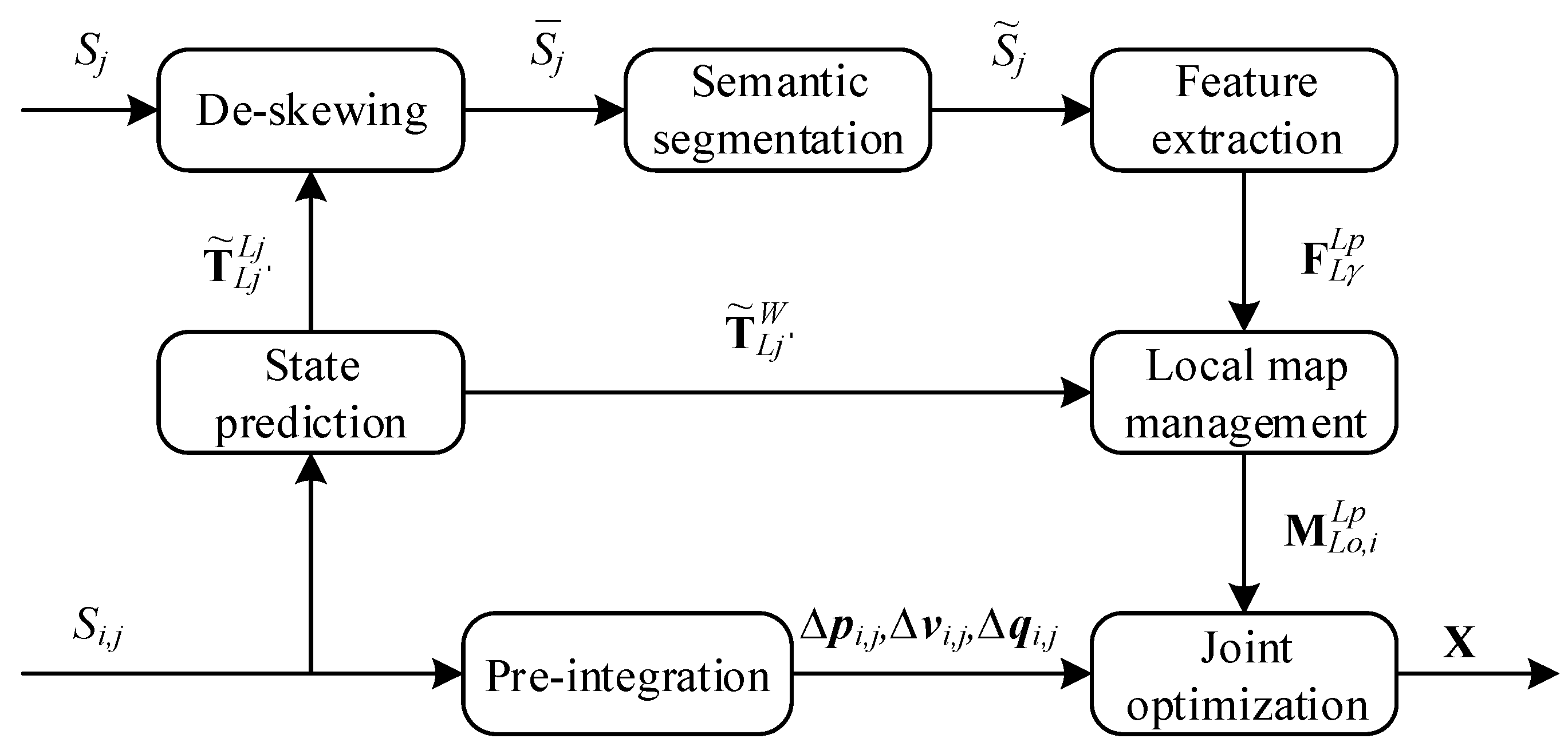
The framework of the proposed semantic lidar-inertial SLAM system is illustrated in Figure 1. Our system is based on LIO-mapping system. IMU measurements $I_{i,j}$ are applied to predict the state of body ${\tilde{T}}_{Lj’}^{Lj}$, which is utilized to de-skew the raw point clouds $S_j$ of lidar data. At the same time, we use IMU pre-integration to obtain pre-integration terms $\Delta {\mathit{p}}_{ij}$, $\Delta {\mathit{v}}_{ij}$, and $\Delta q_{ij}$ for joint non-linear optimization. Then, de-skewed lidar frame ${\overline{S}}_j$ is input into the semantic segmentation network, and we can obtain static point cloud ${\tilde{S}}_j$ after filtering out moving objects. After that, feature points $F_{L\gamma }^{Lp}$ are extracted from several consecutive frames and they are utilized to build local map $M_{Lo,i}^{Lp}$. At last, we use joint non-linear optimization to obtain the final estimation of the states X within a local sliding window.

3.2. State Prediction and Pre-Integration

There are several IMU frames between two consecutive lidar frames. Within a short time, the state of body can be updated by:

$$\begin{array}{l}{\mathit{p}}_j={\mathit{p}}_i+{\displaystyle \sum _{k=i}^{j-1}\left[{\mathit{v}}_k\Delta t+\frac{1}{2}{\mathit{g}}^W\Delta t^2+\frac{1}{2}{R}_k\left({\widehat{\mathit{a}}}_k-{\mathit{b}}_{a_k}\right)\Delta t^2\right]}\\ {\mathit{v}}_j={\mathit{v}}_i+{\mathit{g}}^W\Delta t_{ij}{}^2+{\displaystyle \sum _{k=i}^{j-1}{R}_k\left({\widehat{\mathit{a}}}_k-{\mathit{b}}_{a_k}\right)\Delta t}\\ q_j=q_i\otimes {\displaystyle \prod _{k=i}^{j-1}}\delta q_k=q_i\otimes {\displaystyle \prod _{k=i}^{j-1}}\left[\begin{array}{c}\frac{1}{2}\Delta t\left({\widehat{\mathsf{\omega }}}_k-{\mathit{b}}_{g_k}\right)\\ 1\end{array}\right]\end{array}$$

(1)

where p, v, and q are the position, velocity, and orientation of the IMU body. ${\mathit{b}}_a$ and ${\mathit{b}}_g$ denote acceleration bias and gyroscope bias, respectively. ${\widehat{\mathit{a}}}_k$ and ${\widehat{\mathsf{\omega }}}_k$ are the raw measurements of IMU at timestamp k.

The raw lidar data $S_j$ are skewed because of the lidar sensor’s motion during scanning. So, we de-skew each lidar frame $S_j$ by linear interpolation of ${\tilde{T}}_{Lj’}^{Lj}$ and obtain de-skewed point cloud ${\overline{S}}_j$.

At the same time, the raw IMU outputs ${\widehat{\mathit{a}}}_k$ and ${\widehat{\mathsf{\omega }}}_k$ can be converted to pre-integration measurements ($\Delta {\mathit{p}}_{ij}$, $\Delta {\mathit{v}}_{ij}$, and $\Delta q_{ij}$) by:

$$\begin{array}{l}\Delta {\mathit{p}}_{ij}=R_i^T\left({\mathit{p}}_j-{\mathit{p}}_i-{\mathit{v}}_i\Delta t_{ij}-\frac{1}{2}{\mathit{g}}^W\Delta t_{ij}^2\right)={\displaystyle \sum _{k=i}^{j-1}\left[{\mathit{v}}_{ik}\Delta t+\frac{1}{2}R\left(\Delta q_{ik}\right)\left({\widehat{\mathit{a}}}_k-{\mathit{b}}_{a_k}\right)\Delta t^2\right]}\\ \Delta {\mathit{v}}_{ij}=R_i^T\left({\mathit{v}}_j-{\mathit{v}}_i-{\mathit{g}}^W\Delta t_{ij}^{}\right)={\displaystyle \sum _{k=i}^{j-1}\left[R\left(\Delta q_{ik}\right)\left({\widehat{\mathit{a}}}_k-{\mathit{b}}_{a_k}\right)\Delta t\right]}\\ \Delta q_{ij}=q_i^{-1}\otimes q_j={\displaystyle \prod _{k=i}^{j-1}}\delta q_k={\displaystyle \prod _{k=i}^{j-1}}\left[\begin{array}{c}\frac{1}{2}\Delta t\left({\widehat{\mathsf{\omega }}}_k-{\mathit{b}}_{g_k}\right)\\ 1\end{array}\right]\end{array}$$

(2)

The pre-integration measurements are used for joint optimization.

3.3. Semantic Segmentation Network

We input ${\overline{S}}_j$ into sematic segmentation network to classify it point by point. The semantic segmentation network in our SLAM system is based on PointConv network. The network defines a 3D convolution operation called PointConv:

$$PointConv{\left(S,W,F\right)}_{xyz}={\displaystyle \underset{\left({\delta }_x,{\delta }_y,{\delta }_z\right)\in G}{\iiint }S\left({\delta }_x,{\delta }_y,{\delta }_z\right)W\left({\delta }_x,{\delta }_y,{\delta }_z\right)F\left(x+{\delta }_x,y+{\delta }_y,z+{\delta }_z\right)d}{\delta }_x{\delta }_y{\delta }_z$$

(3)

where $p=\left(x,y,z\right)$ is coordinate of reference point. $\left({\delta }_x,{\delta }_y,{\delta }_z\right)$ is the relative coordinate of any neighbor point from p. $S\left({\delta }_x,{\delta }_y,{\delta }_z\right)$ is the inverse density of point $\left({\delta }_x,{\delta }_y,{\delta }_z\right)$. $W\left({\delta }_x,{\delta }_y,{\delta }_z\right)$ is the weight function. In addition, $F\left(x+{\delta }_x,y+{\delta }_y,z+{\delta }_z\right)$ is the feature of point $\left({\delta }_x,{\delta }_y,{\delta }_z\right)$. The main idea of PointConv is using the relative coordinates of K neighbor points to simulate weight function by multi-layer perceptron (MLP). However, it does not take the features of these neighbor points into consideration.

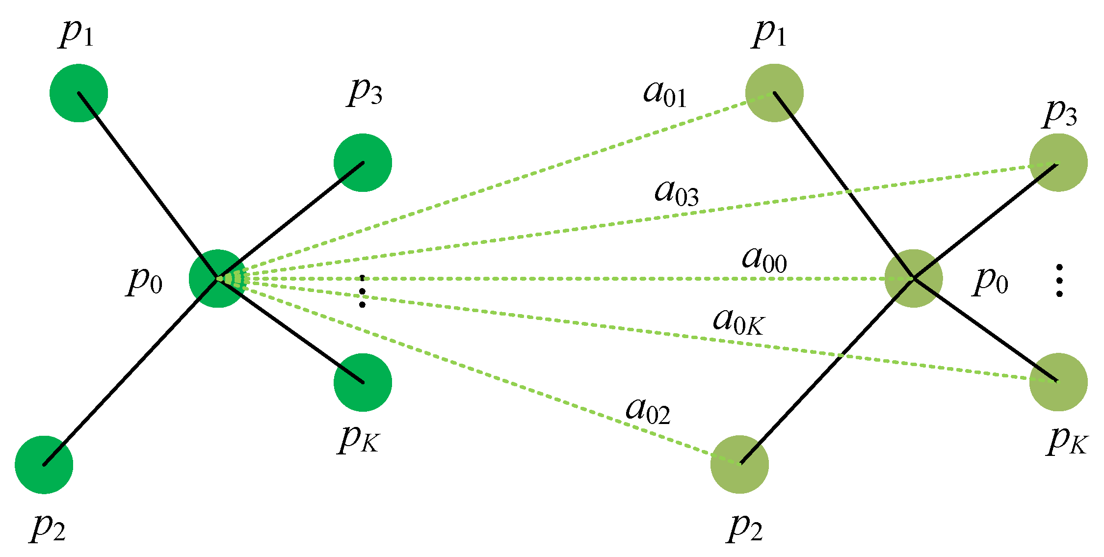
We import an attention mechanism to PointConv and build a graph $G=\left(V,E\right)$ as shown in Figure 2. Given a local point set $P=\left\{p_0,p_1,\dots ,p_K\right\}$, ($f=\left\{f_0,f_1,\dots ,f_K\right\}$ represents the feature of each point), $V\in 0,1,2,\dots ,K$ and $E\in \left|V\right|\times \left|V\right|$ denote the vertices and edges of the graph, respectively. For each point i, the weight between point i and its neighbor point j can be computed by multilayer perceptron:

$${\tilde{a}}_{ij}=MLP\left(\left[\Delta p_{ij}\left|\right|\Delta f_{ij}\right]\right)$$

(4)

where $\Delta p_{ij}=p_j-p_i$, $\Delta f_{ij}=ML{P}_g\left(f_j\right)-ML{P}_g\left(f_i\right)$, and $ML{P}_g$ is also a multilayer perceptron, whose function is mapping a feature from one dimension to another. $\left|\right|$ denotes the concatenation operation.

Therefore, attention weight of the n-th feature channel between point i and its neighbor point j can be computed by:

$$a_{ij,n}=\frac{\exp \left({\tilde{a}}_{ij,n}\right)}{{\displaystyle \sum _{l=0}^K\exp \left({\tilde{a}}_{il,n}\right)}}$$

(5)

The attention feature of point i can be described as:

$$f_i{}^{\prime }={\displaystyle \sum _{j=0}^K{a}_{ij}\ast M_g\left(f_j\right)}+b_i$$

(6)

where $a_{ij}$, $M_g$, and $b_i$ are learnable. ∗ denotes the element-wise production.

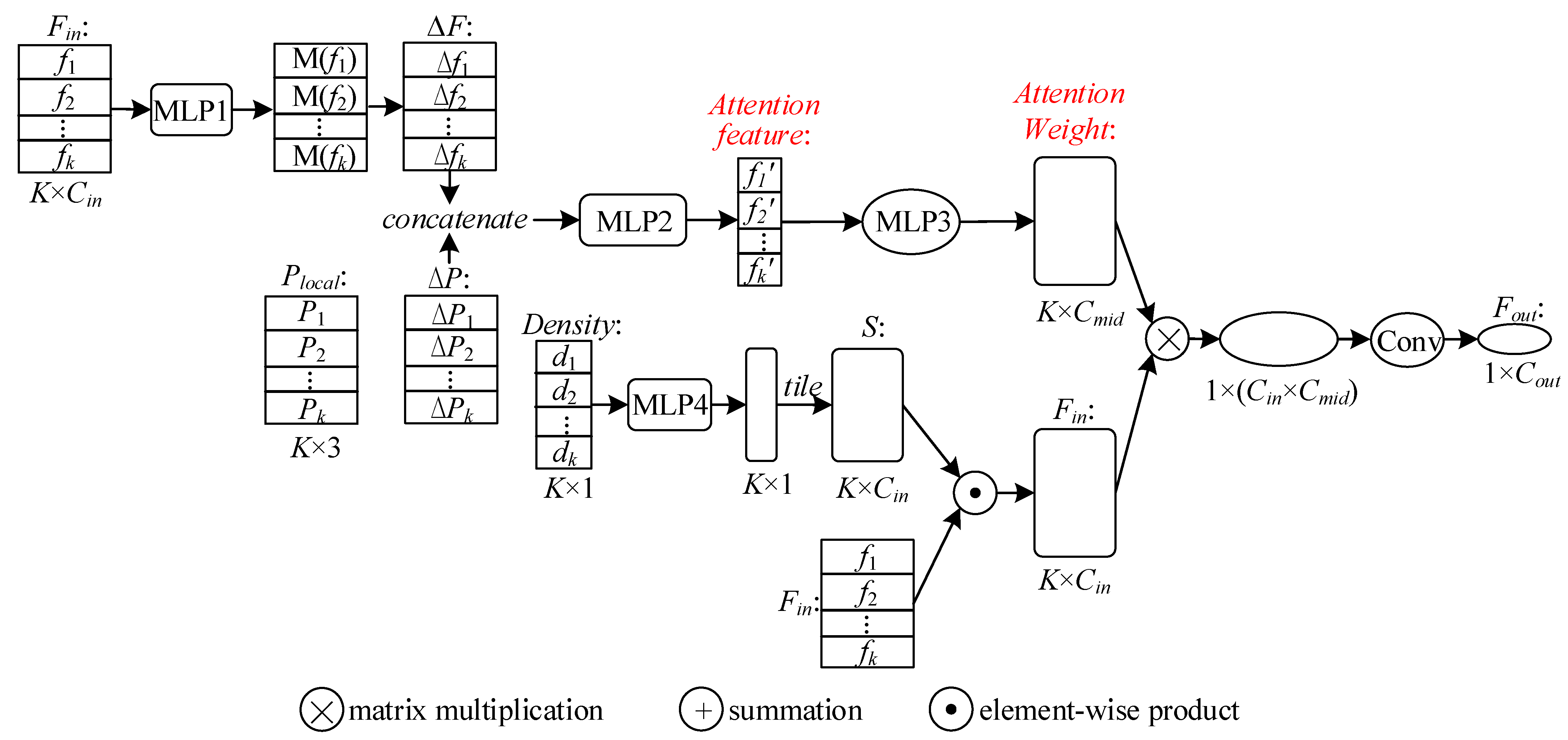
So, for a given local point set $P=\left\{p_0,p_1,p_2,\dots ,p_K\right\}$, we can obtain the attention features through Equation (4). Let $C_{in}$ and ${C^{\prime }}_{in}$ be the number of channels of input feature $f_i$ and output feature $f_i{}^{\prime }$. PointConv only takes the relative coordinate of each point $\left(p_i-p_0\right)$ as inputs to approximate weight function. We extend PointConv by concatenating attention feature $f_i{}^{\prime }$ with $\left(p_i-p_0\right)$, and adopt MLP1 to simulate attention weight function W, as shown in Figure 3. Therefore, the network can focus on the most relevant part of the neighbors to learn features. The entire process of attention PointConv network is shown in Figure 3.

3.4. Feature Extraction and Local Map Management

De-skewed point cloud is segmented through attention PointConv network, and the points belonging to dynamic objects are removed. Then, we adopt lidar feature extraction [19] to select planar feature points, which are most likely on a plane.

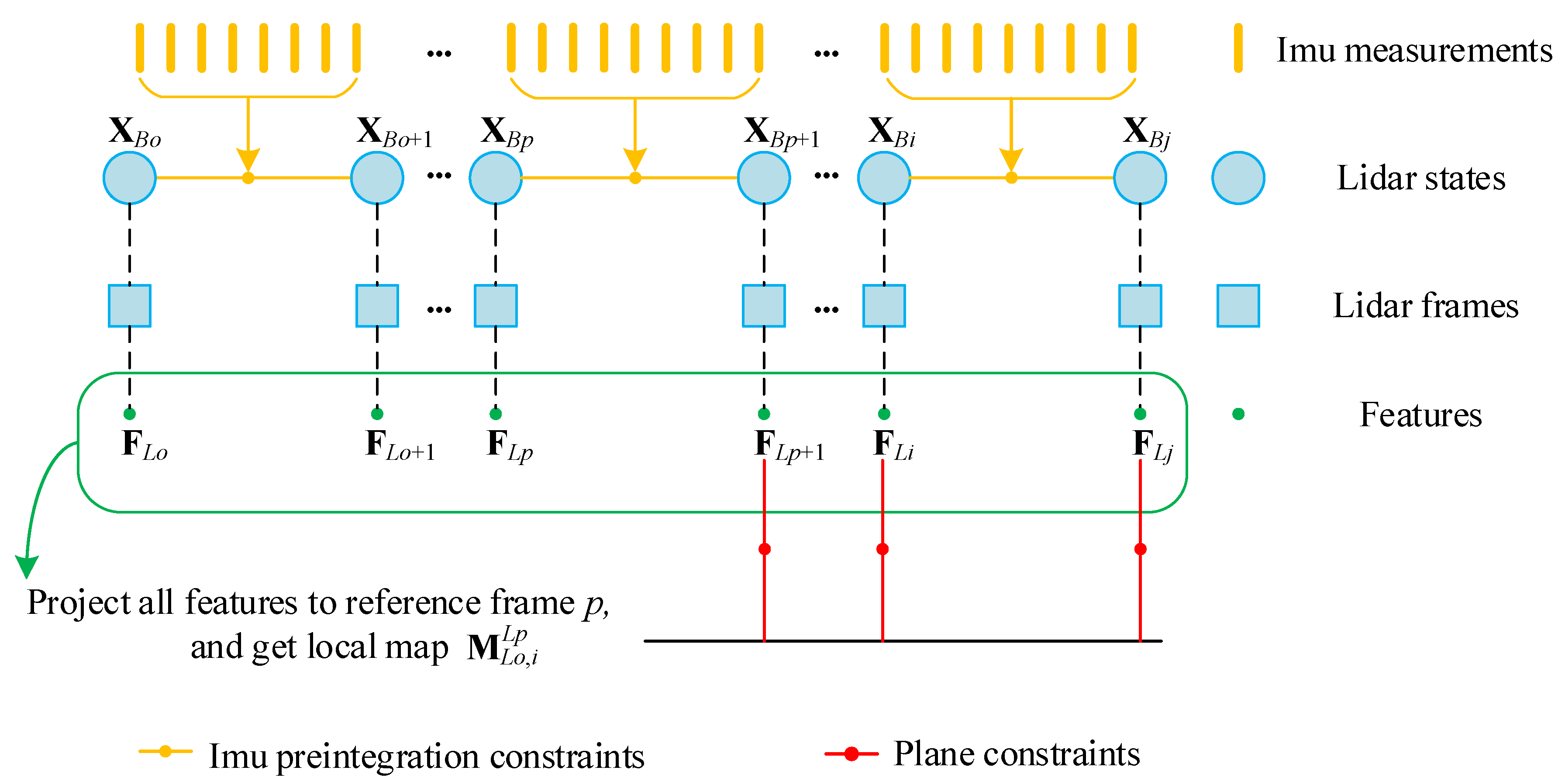
Since one single lidar frame is too sparse for feature matching, we build a local map that consists of feature points of several lidar frames $\left\{o,\cdots ,p,\cdots ,i\right\}$, where o, p, and i are the first frame, the reference frame, and the last frame in the sliding window, respectively, as shown in Figure 4. For $\gamma \in \left\{o,\cdots ,i\right\}$, feature points $F_{L\gamma }$ are projected to reference frame p as $F_{L\gamma }^{Lp}$ and all projected features in the sliding window build a local map $M_{Lo,i}^{Lp}$. The frames before p are already optimized. For each point ${\mathit{x}}^{Lp}\in F_{L\alpha }^{Lp}$ ($\alpha \in \left\{p+1,\cdots ,i,j\right\}$), we adopt KNN algorithm to find its K nearest points $\pi \left({\mathit{x}}^{Lp}\right)$ in $M_{Lo,i}^{Lp}$. Since these K points are most likely on the same plane, they have the plane constraint:

$${\mathit{n}}^T\mathit{x}+d=0, \mathit{x}\in \pi \left({\mathit{x}}^{Lp}\right)$$

(7)

where we denote $m=\left[\mathit{x},\mathit{n},d\right]\in {\mathbf{m}}_{L\alpha }$. In this way, we formulate a relative constraint between the reference frame (n and d are defined in frame p) and the following frames (x is defined in reference α).

3.5. Joint Optimization

Equation (7) provides the constraints between the state of reference frame and the states of following frames. The transformation from the frames to be optimized ($\alpha \in \left\{p+1,\cdots ,i,j\right\}$) to the reference frame p is computed by the chain rule:

$$T_{L\alpha }^{Lp}=T_L^B{T}_{B\alpha }^W{T}_{Bp}^W{}^{-1}{T}_L^B{}^{-1}=\left[\begin{array}{cc}{R}_{L\alpha }^{Lp}& {\mathit{p}}_{L\alpha }^{Lp}\\ 0& 1\end{array}\right]$$

(8)

where $T_L^B$ denotes the extrinsic parameters from lidar to IMU. $T_{B\alpha }^W$ and $T_{Bp}^W$ are the states of the body in frames α and p.

As the window slides, the reference frame also changes. For each $\alpha \in \left\{p+1,\cdots ,i,j\right\}$ and $m=\left[\mathit{x},\mathit{n},d\right]\in m_{L\alpha }$, the residual of Equation (7) can be represented by the distance from point to plane:

$$r_1\left(m,T_{Lp}^W,T_{L\alpha }^W,T_L^B\right)={\mathit{n}}^T\left(R_{L\alpha }^{Lp}\mathit{x}+{\mathit{p}}_{L\alpha }^{Lp}\right)+d$$

(9)

To obtain the states from frame p to frame j, we adopt a joint non-linear optimization and marginalization strategy. As shown in Figure 4, the number of states to be estimated is fixed in the window from $X_{Bp}^W$ to $X_{Bj}^W$. If new constraints appear, the window will include new states and marginalize old states. The entirety of the states in the window can be defined as:

$$X=\left\{X_{Bp}^W,\cdots ,X_{Bj}^W,T_L^B\right\}$$

(10)

State X can be estimated by minimizing the whole cost function:

$$\underset{X}{\min }\frac{1}{2}\left\{{{\displaystyle \sum _{\begin{array}{c}m\in m_{L\alpha }\\ \alpha \in \left\{p+1,\cdots ,j\right\}\end{array}}\Vert r_1\left(m,X\right)\Vert }}^2+{\Vert r_2\left(X\right)\Vert }^2+{\displaystyle \sum _{\beta \in \left\{p,\cdots ,j-1\right\}}{\Vert r_3\left(z_{\beta +1}^{\beta },X\right)\Vert }^2}\right\}$$

(11)

where $r_1\left(m,X\right)$, $r_2\left(X\right)$, and $r_3\left(z_{\beta +1}^{\beta },X\right)$ represent the residual for point-to-plane constraints, marginalization, and IMU pre-integration constraints, respectively. The Gauss–Newton method is used to solve the function above. ${\Vert r_2\left(X\right)\Vert }^2$ is calculated by Schur complement, which is described in [6], and $r_3\left(z_{\beta +1}^{\beta },X\right)$ is computed from the states and IMU pre-integration in [20].

4. Experiments

4.1. Semantic Segmentation Network Training

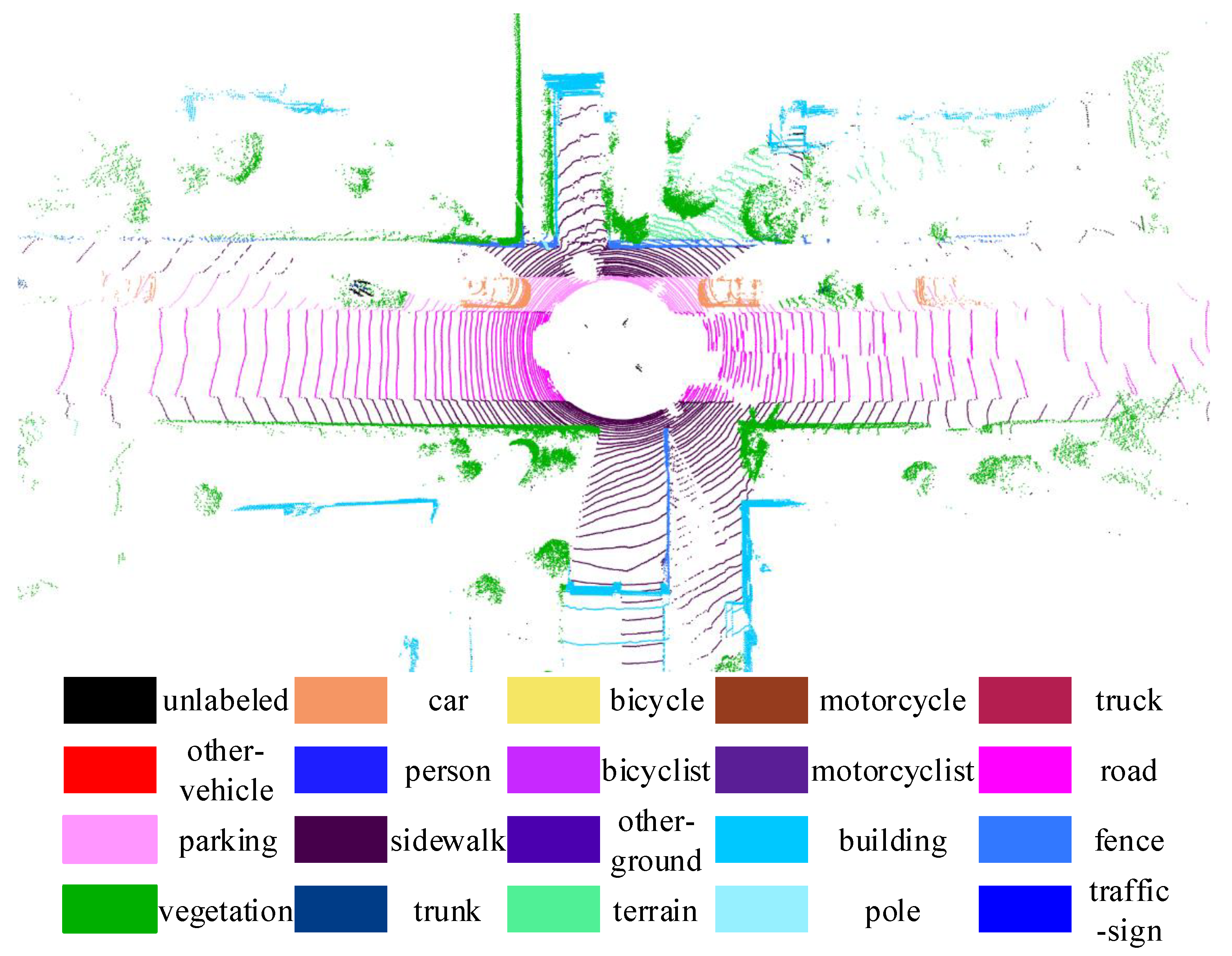
We use the SemanticKITTI dataset to train our attention PointConv network. The semanticKITTI dataset is a large-scale dataset based on the KITTI Vision Benchmark. It provides dense annotations for each individual scan of sequences from 00–10, which enables the usage of multiple sequential scans for semantic segmentation. Labels for the test set (sequences 11–21) are not provided. Figure 5 shows a single lidar frame with semantic annotations of the SemanticKITTI dataset, and it contains 20 classes including classes distinguishing non-moving and moving objects.

We train our attention PointConv network with all the scans of sequences 00–10. In addition, in the next section, we will show the semantic segmentation results of our trained network.

4.2. Dynamic Object Removal

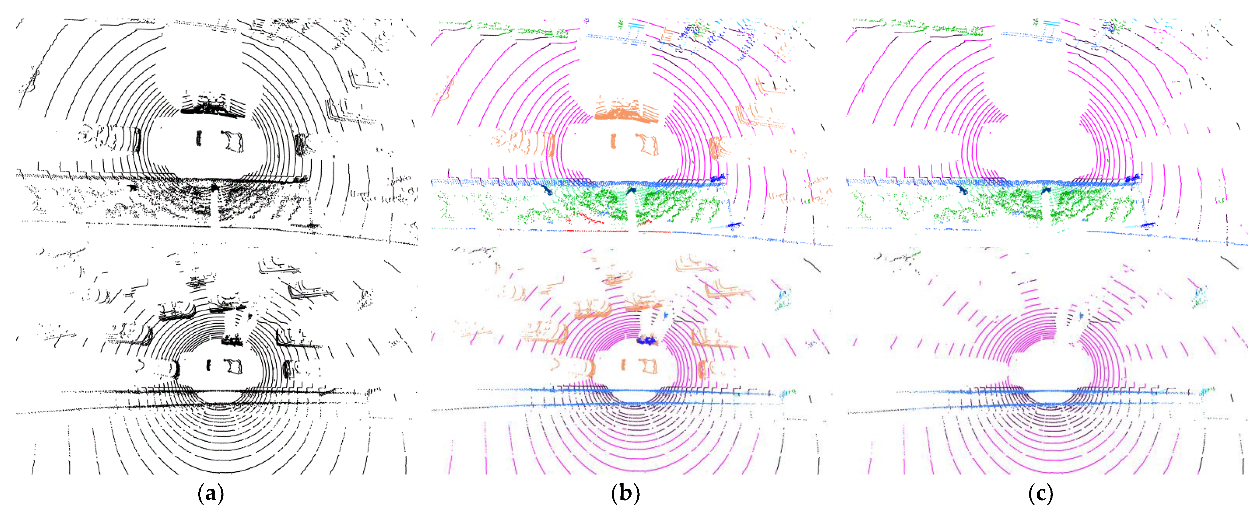
We use UrbanNav datasets to test the performance of the dynamic object removal. UrbanNav datasets are collected by mounting the data collection platform on a Honda Fit. The platform is equipped with Velodyne HDL-32E lidar, an Xsens Mti-10 IMU, a monocular camera, and a SPAN-CPT (for ground truth). Two lidar scan samples are shown in Figure 6a. Each lidar frame is input to our attention PointConv network to obtain point-wise labels, as shown in Figure 6b. Then, we filter out the points belonging to dynamic labels and obtain static point clouds, as in Figure 6c. From the visualization of the point cloud samples, we can see that the annotations of the points are basically correct, and the removal of the dynamic objects is effective.

4.3. Pose Estimation Comparison

In this section, we compare the accuracy and robustness of the proposed method with the current state-of-the-art lidar-inertial SLAM methods, including LIO-mapping, LINS, and LIO-SAM. LINS is a filter-based tightly coupled method, and LIO-SAM is a tightly coupled method based on nonlinear optimization.

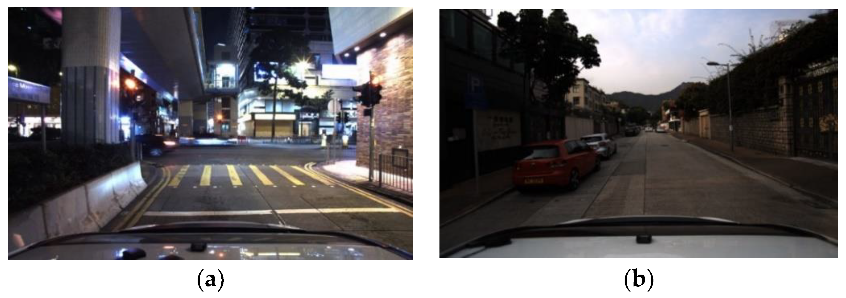
We also use UrbanNav datasets to compare the performance of different methods. Specifically, we used the Urban2019 dataset and Urban2020 dataset. The former was gathered in a typical urban canyon of Hong Kong featuring high-rising buildings and numerous dynamic objects in the evening. The latter was gathered in a low-urbanization area in Hong Kong with some dynamic objects present during in the day, as shown in Figure 7.

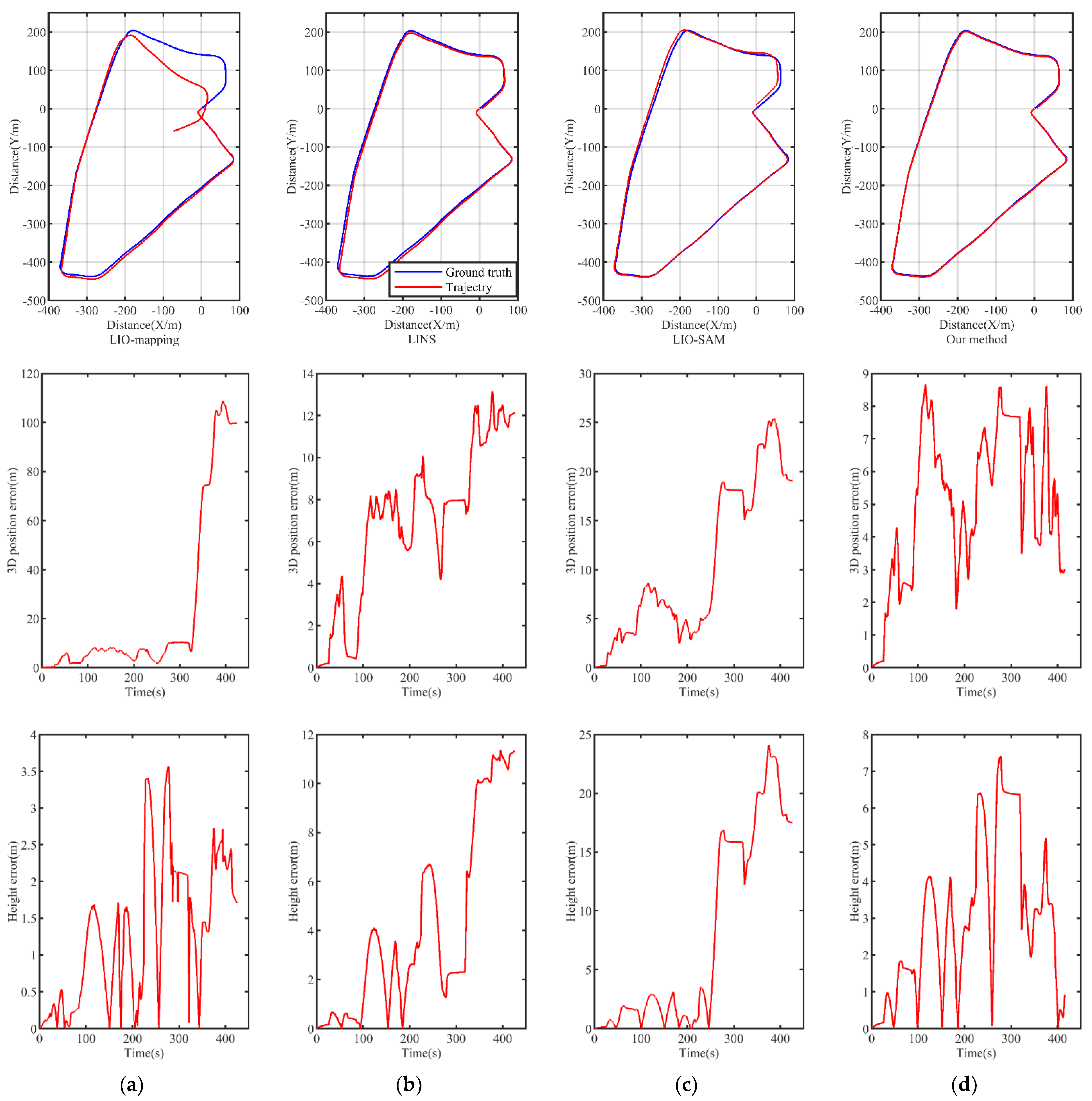
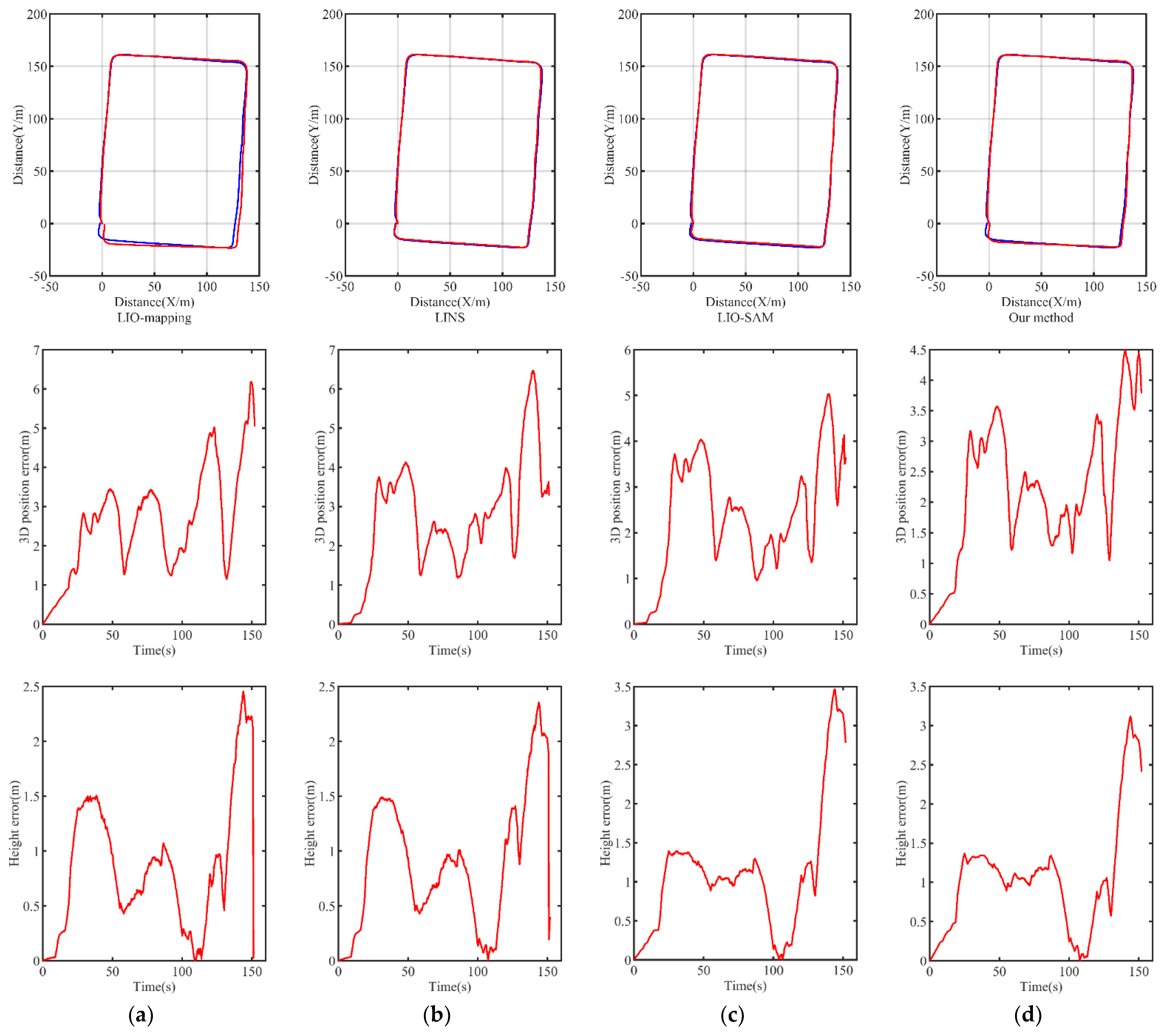
In this experiment, the datasets start and end at the origin. The GPS measurements of the datasets serve as the ground truth. The estimated trajectories of various methods applied to the Urban2019 dataset are shown in Figure 8. LIO-mapping performs well at the beginning of the dataset, but it drifts later in the trajectory and the rotation of LIO-mapping deviates at the curve. This is mainly caused by false feature points belonging to dynamic objects. The trajectories of LINS and LIO-SAM have a similar degree of misalignment, and they both have a slight deviation from the start point to the end point. The overall trajectory of the proposed method performs well.

Furthermore, we display the 3D position errors and height errors of the different methods with respect to time in Figure 8. The 3D position errors and height errors of the three other methods increase dramatically at one certain point. The 3D position errors of the LIO-mapping approach reach up to more than 100 m, which means that the algorithm has totally failed. By contrast, the 3D position error and height error of our method fluctuate within a certain section since errors accumulate more slowly after moving dynamic objects.

The estimated trajectories of the Urban2020 dataset are demonstrated in Figure 9. As shown, all the methods perform better than they did for the Urban2019 dataset, as there are fewer dynamic objects on the road and the distance is shorter. Even so, the proposed method performs better than the LIO-mapping approach with respect to the trajectory. In addition, the 3D position errors and height errors are also lower.

Table 1. The end-to-end translation errors, end-to-end rotation errors, and RMSE errors of different methods on both datasets.

Dataset	Error Type	LIO-Mapping	LINS	LIO-SAM	Our Method
Urban2019	Translation (m)	95.473	13.258	19.274	5.673
	Rotation (degree)	22.829	24.704	16.942	14.554
	RMSE (m)	43.018	7.863	13.069	5.543
Urban2020	Translation (m)	5.030	1.276	3.513	3.713
	Rotation (degree)	14.626	25.092	6.556	7.670
	RMSE (m)	3.107	3.039	2.672	2.625

displays the end-to-end translation errors, end-to-end rotation errors, and RMSE errors with regard to the ground truth. Our method achieves the lowest RMSE error on both datasets. Furthermore, our method is superior to LIO-mapping with respect to end-to-end translation and rotation errors.

4.4. Runtime Performance Evaluation

In this section, we will show the average runtime of each module of our algorithm. The algorithm was tested with a 2.6-GHz i7-9720H CPU and an Nvidia GeForce GTX 1660 Ti GPU in Ubuntu 18.04. We downsampled the point cloud of each lidar frame by using a voxelgrid filter whose leaf size is 0.5 m. The average runtime of each module is presented in

Table 2. Average runtime of each module (ms).

Dataset	Prediction	Semantic Segmentation	Odometry	Laser Mapping
Urban2019	0.00928	106.8	126.5	201.9
Urban2020	0.01198	122.6	127.9	252.8

, and all the modules run on different threads.

4.5. Global Map Comparison

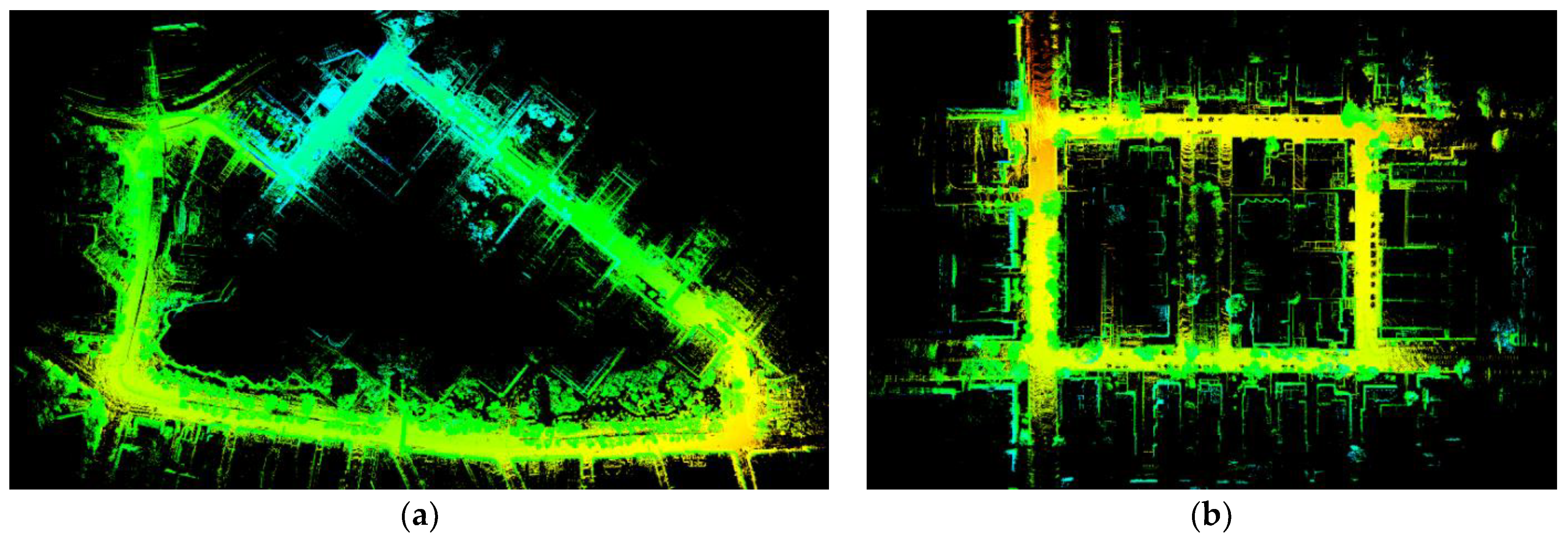
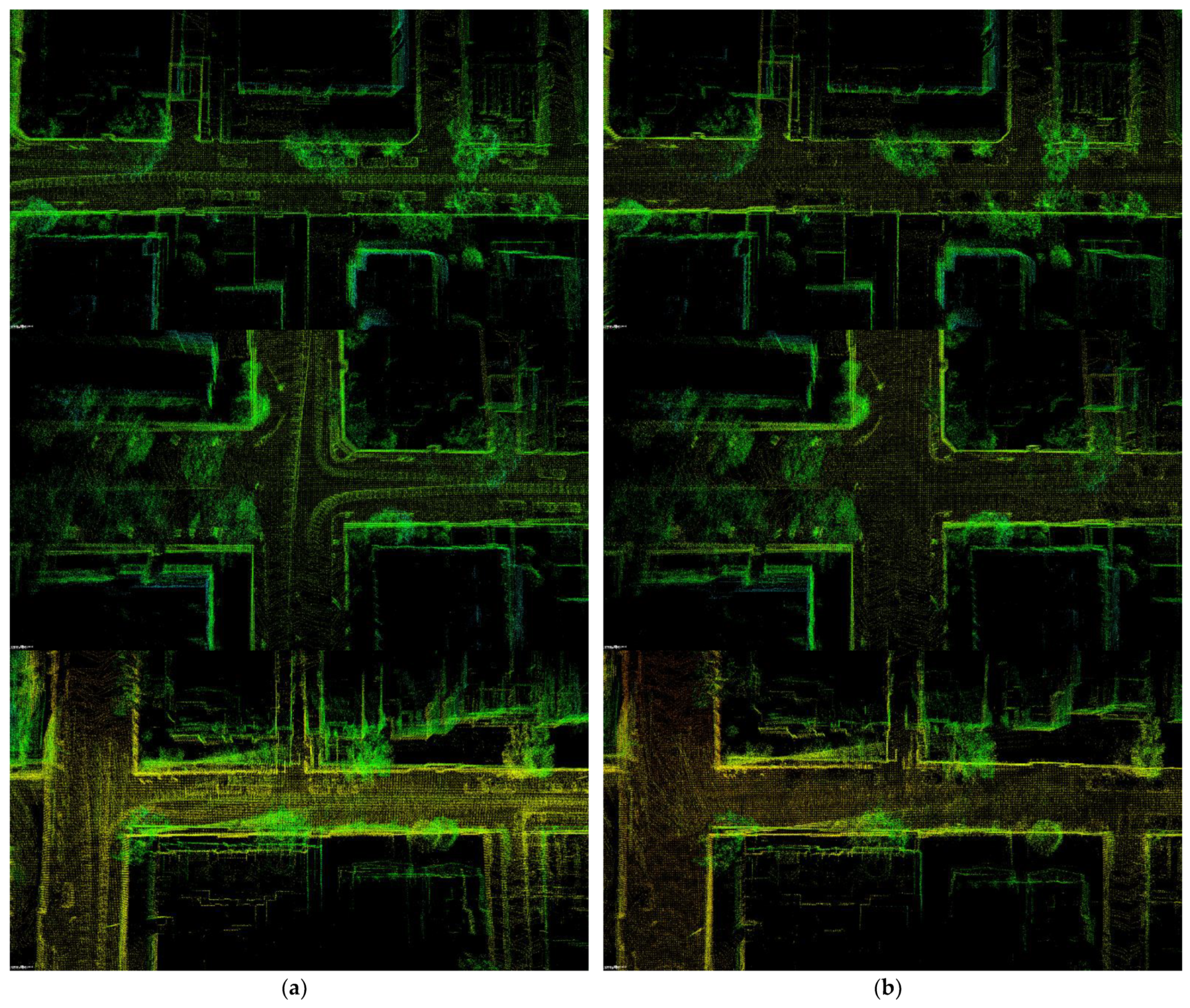
Finally, we test the performance of the global map built using our method. The global maps of the proposed method applied to the Urban2019 dataset and Urban2020 dataset are illuminated in Figure 10a,b). It is shown that the global maps of our method are basically correct. To compare the maps built by the LIO-mapping method and our method, we focus on several parts of the map in Figure 11. Figure 11a corresponds to LIO mapping and Figure 11b to our method. The figures demonstrate that our method can eliminate dynamic objects including vehicles of all kinds, which are meaningless for a global map. Furthermore, Figure 11a shows many obvious trails of the speeding vehicles on the roads, while the same roads in Figure 11b are clean, because the points belonging to moving cars have been filtered out in each lidar frame.

5. Conclusions

Most SLAM systems work on the assumption that the environment is static. In this paper, we have proposed a semantic lidar-inertial SLAM system for dynamic scenes. We imported an attention mechanism to the PointConv network to elevate the feature-learning capability of the network. The LIO-mapping system was combined with an attention PointConv semantic segmentation network, and the points belonging to dynamic objects were removed in each lidar frame. The stable static feature points were extracted, and a static local map was built to perform ego-motion estimation. The experiments demonstrate that our method can decrease the errors of the estimated trajectories and build a clear global map of dynamic scenes.

References

- Cadena, C.; Carlone, L.; Carrillo, H.; Latif, Y.; Scaramuzza, D.; Neira, J.; Reid, I.; Leonard, J.J. Past, Present, and Future of Simultaneous Localization and Mapping: Toward the Robust-Perception Age. IEEE Trans. Robot. 2016, 32, 1309–1332. [Google Scholar] [CrossRef] [Green Version]
- Grisetti, G.; Kümmerle, R.; Stachniss, C.; Burgard, W. A Tutorial on Graph-Based SLAM. IEEE Intell. Transp. Syst. Mag. 2010, 2, 31–43. [Google Scholar] [CrossRef]
- Ji, K.; Chen, H.; Di, H.; Gong, J.; Xiong, G.; Qi, J.; Yi, T. CPFG-SLAM: A robust simultaneous localization and mapping based onLIDAR in off-road environment. In Proceedings of the 2018 IEEE Intelligent Vehicles Symposium (IV), Changshu, China, 26–30 June 2018. [Google Scholar]
- Zhang, J.; Singh, S. Loam: Lidar odometry and mapping in real-time. In Proceedings of the 2014 Robotics: Science and Systems, Berkeley, CA, USA, 12–16 July 2014. [Google Scholar]
- Shan, T.; Englot, B. Lego-loam: Lightweight and ground-optimized lidar odometry and mapping on variable terrain. In Proceedings of the 2018 IEEE/RSJ International Conference on Intelligent Robots and Systems (IROS), Madrid, Spain, 1–5 October 2018. [Google Scholar]
- Ye, H.; Chen, Y.; Liu, M. Tightly Coupled 3D Lidar Inertial Odometry and Mapping. In Proceedings of the 2019 IEEE International Conference on Robotics and Automation, Montreal, QC, Canada, 20–24 May 2019. [Google Scholar]
- Qin, C.; Ye, H.; Pranata, C.E.; Han, J.; Zhang, S.; Liu, M. LINS: A Lidar-Inertial State Estimator for Robust and Efficient Navigation. In Proceedings of the 2020 IEEE International Conference on Robotics and Automation (ICRA), Paris, France, 31 May 2020–31 August 2020. [Google Scholar]
- Shan, T.; Englot, B.; Meyers, D.; Wang, W.; Ratti, C.; Rus, D. LIO-SAM: Tightly-coupled Lidar Inertial Odometry via Smoothing and Mapping. In Proceedings of the 2020 IEEE/RSJ International Conference on Intelligent Robots and Systems (IROS), Las Vegas, NV, USA, 24 October 2020–24 January 2021. [Google Scholar]
- Behley, J.; Stachniss, C. Efficient Surfel-Based SLAM using 3D Laser Range Data in Urban Environments. In Proceedings of the 2018 Robotics: Science and Systems, Pittsburgh, PA, USA, 26–30 June 2018. [Google Scholar]
- Wu, W.; Qi, Z.; Li, F. PointConv: Deep Convolutional Networks on 3D Point Clouds. In Proceedings of the 2019 IEEE Conference on Computer Vision and Pattern Recognition (CVPR), Long Beach, NY, USA, 15–20 June 2019. [Google Scholar]
- Behley, J.; Garbade, M.; Milioto, A.; Quenzel, J.; Behnke, S.; Stachniss, C.; Gall, J. SemanticKITTI: A dataset for semantic scene understanding of LiDAR sequences. arXiv 2020, arXiv:1904.01416. [Google Scholar]
- Hsu, L.-T.; Kubo, N.; Wen, W.; Chen, W.; Liu, Z.; Suzuki, T.; Meguro, J. UrbanNav: An Open-Sourced Multisensory Dataset for Benchmarking Positioning Algorithms Designed for Urban Areas. In Proceedings of the 34th International Technical Meeting of the Satellite Division of the Institute of Navigation (ION GNSS+), St. Louis, MO, USA, 20–24 September, 2021. [Google Scholar]
- Yu, C.; Liu, Z.; Liu, X.; Xie, F.; Yang, Y.; Wei, Q.; Fei, Q. DS-SLAM: A Semantic Visual SLAM towards Dynamic Environments. In Proceedings of the 2018 IEEE/RSJ International Conference on Intelligent Robots and Systems (IROS), Madrid, Spain, 1–5 October 2018. [Google Scholar]
- Bescos, B.; Fcil, J.M.; Civera, J.; Neira, J. DynaSLAM: Tracking, Mapping, and Inpainting in Dynamic Scenes. IEEE Robot. Autom. Lett. 2018, 3, 4076–4083. [Google Scholar] [CrossRef] [Green Version]
- Mur-Artal, R.; Tardós, J.D. ORB-SLAM2: An Open-Source SLAM System for Monocular, Stereo, and RGB-D Cameras. IEEE Trans. Robot. 2017, 33, 1255–1262. [Google Scholar] [CrossRef] [Green Version]
- Chen, X.; Milioto, A.; Palazzolo, E.; Giguere, P.; Behley, J.; Stachniss, C. SuMa++: Efficient LiDAR-based semantic SLAM. In Proceedings of the 2019 IEEE/RSJ International Conference on Intelligent Robots and Systems (IROS), Macau, China, 3–8 November 2019. [Google Scholar]
- Li, L.; Kong, X.; Zhao, X.; Li, W.; Wen, F.; Zhang, H.; Liu, Y. SA-LOAM: Semantic-aided LiDAR SLAM with Loop Closure. arXiv 2021, arXiv:2106.11516. [Google Scholar]
- Wang, W.; You, X.; Zhang, X.; Chen, L.; Zhang, L.; Liu, X. LiDAR-Based SLAM under Semantic Constraints in Dynamic Environments. Remote Sens. 2021, 13, 3651. [Google Scholar] [CrossRef]
- Bosse, M.; Zlot, R. Continuous 3d scan-matching with a spinning 2d laser. In Proceedings of the 2009 IEEE International Conference on Robotics and Automation, Kobe, Japan, 12–17 May 2009. [Google Scholar]
- Qin, T.; Li, P.; Shen, S. Vins-mono: A robust and versatile monocular visual-inertial state estimator. IEEE Trans. Robot. 2018, 34, 1004–1020. [Google Scholar] [CrossRef]
Figure 1.
Overall framework of the proposed semantic lidar-inertial SLAM.
Figure 2.
Illustration of attention mechanism on a reference point. The weight function is a weighted combination of the neighbors.
Figure 3.
The whole process of attention PointConv network.
Figure 4.
Illustration of sliding window and local map.
Figure 5.
A single scan with labels of SemanticKITTI dataset.
Figure 6.
(a) the original point clouds; (b) semantic segmentation results with point-wise labels; (c) point clouds after filtering out dynamic points.
Figure 7.
Sample images of datasets: (a) Urban2019 dataset; (b) Urban2020 dataset.
Figure 8.
Estimated trajectories, 3D position errors, and height errors of different methods applied to Urban2019 dataset: (a) LIO−mapping; (b) LINS; (c) LIO−SAM; (d) our method.
Figure 9.
Estimated trajectories, 3D position errors, and height errors of different methods in Urban2020 dataset: (a) LIO−mapping; (b) LINS; (c) LIO−SAM; (d) our method.
Figure 10.
Global map built using the proposed method: (a) Urban2019 dataset; (b) Urban2020 dataset.
Figure 11.
Detailed parts of global map created using LIO mapping and our method: (a) corresponds to LIO-mapping method; (b) corresponds to our method.