Article

Balance Control of a Configurable Inverted Pendulum on an Omni-Directional Wheeled Mobile Robot

Department of Engineering Science, National Cheng Kung University, Tainan City 701401, Taiwan
*
Author to whom correspondence should be addressed.
Appl. Sci. 2022, 12(20), 10307; https://doi.org/10.3390/app122010307
Submission received: 19 September 2022 / Revised: 6 October 2022 / Accepted: 8 October 2022 / Published: 13 October 2022
(This article belongs to the Special Issue New Trends in Robotics, Automation and Mechatronics (RAM))

Abstract

:
This paper considers the balance control problems of a configurable inverted pendulum with an omni-directional wheeled mobile robot. The system consists of two parts. One is an inverted pendulum, and another one is an omni-directional wheeled mobile robot. The system can be configured as a rotary inverted pendulum or a spherical inverted pendulum. The objective is to control the omni-directional wheeled mobile robot to provide translational force on the plane to balance the spherical inverted pendulum and to provide the moment to balance the rotary inverted pendulum. Detailed dynamic models of these two systems are derived for the control strategy design and simulation studies. Stabilizing controllers based on the second-order sliding mode control are designed for both systems. The closed-loop stability is proved based on the passivity properties. The proposed control schemes can guarantee semi-globally asymptotical stability over the upper-half plane. In addition, the conventional sliding mode controllers proposed in our previous work and Linear-Quadratic Regulator (LQR) controllers based on the linearized system models about its upright equilibrium point are also used for performance comparison. The effectiveness of the control strategies is investigated and verified using simulation and experimental studies. In the simulation studies, different sources of uncertainty and disturbance are investigated. It is shown that the second-order sliding mode control outperforms the conventional sliding mode control and LQR control without any uncertainty and disturbance. For robustness to the matched disturbance, the simulation results show that the second-order sliding mode controller has a less significant steady-state oscillation in the pendulum’s angular displacement than other controllers. The simulation results also show that only the second-order sliding mode controller can stabilize the system with a significant initial deviation from the pendulum’s upright position. Finally, the experimental results demonstrate that second-order sliding mode control outperforms conventional sliding mode control and LQR control.

1. Introduction

The inverted pendulum model can be found in many engineering applications such as walking robots [1], personal transporter [2], and single-wheeled mobile robot [3]. The dynamics of an inverted pendulum are inherently open loop unstable, nonlinear, underactuated, and non-minimum phase, so balance control of the inverted pendulum is a formidable challenge. It is widely used as a benchmark for designing and validating different control techniques. Due to its importance in control engineering, the inverted pendulum has been often used in control education for many decades. For research and education on the control, several variants of inverted pendulum systems with distinct mechanism constructions and actuation have been proposed and studied, such as rotary inverted pendulum [4], Acrobot [5], Pendubot [6], inertia wheel pendulum [7], cart-pole inverted pendulum [8], double inverted pendulum [9], triple-link inverted pendulum [10], and spherical inverted pendulum [11,12], etc. The omni-directional wheeled mobile robot [13,14] is a particular class of wheeled mobile robots. This robot uses orthogonal omni-directional wheels, which provide traction in the direction normal to the wheel shaft, and the wheel can slide passively in the direction of the wheel shaft. This mobile robot does not have nonholonomic constraints and can simultaneously perform translational movement along an arbitrary trajectory combined with any orientation. In [15], an omni-directional wheeled mobile robot was used to generate the planar control force for balancing a spherical inverted pendulum.
This paper uses second-order sliding mode control [16] to stabilize the inverted pendulum systems. Sliding mode control has been known as a robust and nonlinear control technique appropriate for compensating matched uncertainties and disturbances in dynamical systems [16,17]. Essentially, the state trajectories of the closed-loop system are constrained to a specific manifold in the state space in finite time and to retain their motion to slide along the specific manifold for all successive times when sliding mode control uses switching control actions. The closed-loop system is insensitive to external disturbances and model uncertainties because the motion of the state trajectory is constrained on a predefined sliding manifold. The chattering behavior [17] is the main obstacle for the practical application in the conventional or first-order sliding mode control. The chattering problems can be effectively attenuated using higher-order sliding mode controls [16,18] with a relative degree two or higher. Another merit is that higher-order sliding mode control extends the relative degree of the sliding variable in the conventional sliding mode control from one to a higher order. Due to its simplicity and low information demand, second-order sliding mode control is the most widely used in practice [19,20,21] among the higher-order sliding mode control.
This paper considers the problems of the control design and experimental validation of balance control of a configurable inverted pendulum system with an omni-directional wheeled mobile robot. This system can be configured as a rotary inverted pendulum system or a spherical inverted pendulum system. The omni-directional wheeled mobile generates the designed control torque for balancing the rotary inverted pendulum and the designed control planar force for balancing the spherical inverted pendulum. Figure 1 is the schematic diagram of the proposed system, (a) is a rotary inverted pendulum system, and (b) is a spherical inverted pendulum system. For simulation and control design, mathematical models of omni-directional wheeled mobile robot and both inverted pendulums are derived. To enhance robustness to model uncertainties and disturbance, a coupled sliding manifold [22] and second-order sliding mode control are applied to design stabilizing controllers for both inverted pendulum systems. The closed-loop stability is proved based on the passivity properties of the zero dynamics of the system confined on the sliding manifold. It is shown that the closed-loop system can be semi-globally asymptotically stabilized over the upper-half plane. A sufficient condition is derived to guarantee the semi-globally asymptotical stability of the closed-loop system. The experimental setup is built for experimental validation and performance evaluation of the designed control laws. Furthermore, for the performance comparison, conventional sliding mode controllers proposed in our previous work [15] and LQR controllers [23] for the linearized system models are also used.
The organization of this research is as below: In Section 2, the dynamic models of an omni-directional wheeled mobile robot, a rotary inverted pendulum, and a spherical inverted pendulum are presented. In Section 3, the design of the controllers for stabilizing the systems and stability analysis of the closed-loop system are given. Section 4 describes the experimental setup. Section 5 presents the results of simulations and experiments. Finally, Section 6 contains some concluding remarks.

2. Mathematical Modeling

The system dynamics can be divided into two parts: one is the actuation subsystem, and the other is an inverted pendulum subsystem. The actuation subsystem is an omni-directional wheeled mobile robot. The system can be configured as two types of the inverted pendulum subsystems, namely rotary inverted pendulum and spherical inverted pendulum. In this section, mathematical models will be established for the actuation subsystem and each inverted pendulum subsystem and finally, from the system model of the mobile robot, the forces and torque generated by the mobile robot for controlling the inverted pendulum subsystems are given in terms of the motor control voltages.

2.1. Model of an Omni-Directional Wheeled Mobile Robot

Here is a mathematical model derived for an omni-directional wheeled mobile robot using Newton’s laws [24]. This mobile robot consists of a rigid circular chassis and three omni-directional wheels labeled 1, 2, and 3. The wheels were arranged at an equal distance from the center of the robot chassis and equally spaced at 120 . All wheels are assumed to roll without slip. Figure 2 illustrates the basic features of an omni-directional wheeled mobile robot from the top view.
The system variables and parameters are defined as below:
O ^ W , X ^ W , Y ^ W : world   coordinate   system . O ^ M , X ^ M , Y ^ M : body   coordinate   system   with   the   origin   attached   to   the   center   of   mass     of   the   mobile   robot ,   and   the   Y ^ M - axis   is   aligned   to   wheel   1 . M t : mass   of   the   mobile   robot   with   the   pendulum . f 1 , f 2 , f 3 : reaction   force   applied   by   the   ground   to   the   omni - directional   wheel ,     where   the   direction   is   vertical   to   wheel   axes   1 ,   2 ,   and   3 ,   respectively . L c : radius   of   the   mobile   robot . R w : radius   of   the   omni - directional   wheels . δ c : angle   between   wheel   2   and   the   X ^ M - axis   of   the   mobile   coordinate     system ;   the   value   is   fixed   to   30 ° . I c z z : the   mobile   robot s   moment   of   inertia   about   the   Z ^ M - axis . ϕ : rotation   angle   of   the   mobile   robot . θ 1 , θ 2 , θ 3 : rotation   angle   of   omni - directional   wheels   1 ,   2 ,   and   3 ,   respectively . ω 1 , ω 2 , ω 3 : angular   velocity   of   omni - directional   wheels   1 ,   2 ,   and   3 ,   respectively . x W y W T : position   for   the   center   of   mass   of   the   robot   relative   to   the   world     coordinate   system .
The dynamic and kinematic equations of the omni-directional wheeled mobile robot are given by
x ¨ W y ¨ W ϕ ¨ = M t 0 0 0 M t 0 0 0 I y cos ϕ sin ϕ 0 sin ϕ cos ϕ 0 0 0 1 1 1 2 1 2 0 3 2 3 2 L c L c L c f 1 f 2 f 3
θ ˙ 1 θ ˙ 2 θ ˙ 3 = ω 1 ω 2 ω 3 = 1 R w 1 0 L c 1 2 3 2 L c 1 2 3 2 L c cos ϕ sin ϕ 0 sin ϕ cos ϕ 0 0 0 1 x ˙ W y ˙ W ϕ ˙
Because the electrical time constant of a motor is usually far less than the mechanical time constant, the relationship between the motor torque τ m and control voltage u is hence based on the reduced-order model of a DC motor and is given blow
τ m = K t R a u K t 2 R a ω m ,
where R a is the armature resistance, K t is the motor torque constant, u is the control voltage and ω m is the angular velocity of the motor. These unmodeled dynamics of the motor can then be considered as the matched uncertainty [16,17] in the control design. The relationship between the motor torque and the wheel force f acting on the robot is given by
f = 1 R w τ m .
The three motors used in this mobile robot are assumed to be identical. Therefore, combining (3) and (4), the relationship between f, u, and ω of three motors are given by
f 1 f 2 f 3 = n K t R w R a u 1 u 2 u 3 n 2 K t 2 R w R a ω 1 ω 2 ω 3
where u 1 , u 2 , u 3 are motor control voltages. From (1), (2), and (5), the dynamics of the robot in the world frame can be re-written as
P ¨ w = A w P ˙ w + B w ( ϕ ) U C ,
where
P w = [ x W y W ϕ ] T , A w = a 1 0 0 0 a 1 0 0 0 a 2 , U C = [ u 1 u 2 u 3 ] T , B w ( ϕ ) = 2 b 1 cos ( ϕ ) b 1 cos ( ϕ ) 3 b 1 sin ( ϕ ) b 1 cos ( ϕ ) + 3 b 1 sin ( ϕ ) 2 b 1 sin ( ϕ ) b 1 sin ( ϕ ) + 3 b 1 cos ( ϕ ) b 1 sin ( ϕ ) 3 b 1 cos ( ϕ ) b 2 b 2 b 2 ,
with
a 1 = 3 K t 2 2 R w 2 M t R a , a 2 = 3 K t 2 L c 2 R w 2 I c z z R a , b 1 = K t 2 R w M t R a , b 2 = K t L c R w I c z z R a .

2.2. Model of a Rotary Inverted Pendulum

The mathematical modeling of a rotating inverted pendulum as shown in Figure 3 will be described in this subsection. Here the pendulum rod is mounted to a pivot point off the robot’s center. The pendulum rod can rotate freely in the vertical plane perpendicular to the axis connecting the center of the robot and the pivot point. The world frame is denoted by the coordinate system O ^ W X ^ W Y ^ W Z ^ W , the origin O ^ W coincides with the center of mass of the robot, the X ^ W -axis aligns with the X ^ M -axis of the robot, and the Y ^ W -axis aligns with Y ^ M -axis of the robot. The pendulum’s body frame is o x y z , the origin o coincides with the pivot point of the inverted pendulum, the z -axis aligns with the pendulum, and the x -axis aligns with the vector O ^ W o ¯ .
The system variables and parameters are defined as below:
m : the   pendulum   mass . l : length   of   the   pendulum   from   its   center   of   mass   to   the   pivot   point . β : the   pendulum s   angular   displacement   from   the   vertical   upright . ϕ : the   robot s   rotational   angular   displacement . I p x x , I p y y , I p z z : the   pendulum s   moment   of   the   inertia   about   the x - axis , y - axis ,   z - axis ,     respectively . R c : distance   from   the   pivot   point   of   the   pendulum   to   the   center   of   the   robot . g : gravitational   acceleration . I c z z : the   robot s   moment   of   the   inertia   about   the   Z ^ W - axis . τ ϕ : torque   exerted   by   the   robot .
Assuming that the robot is controlled to have the rotational motion only. For the derivation of the system dynamic equations, the Euler-Lagrange method [24] was used. The form of the Euler-Lagrange equations is
d d t L q ˙ L q = Q ,
where Q is the generalized forces, and q is the generalized coordinates, and L is the Lagrangian function which is defined as
L = T V ,
where T is the kinetic energy and V is the potential energy. For this system, q is selected as
q = β ϕ T ,
Q is given by
Q = 0 τ ϕ T .
From (7), the dynamic equations are given by
( m l 2 + I p x x ) β ¨ + m l R c cos β ϕ ¨ + ( I p z z m l 2 I p y y ) sin β cos β ϕ ˙ 2 m g l sin β = 0 ,
m l R c cos β β ¨ + ( m l 2 sin 2 β + m R c 2 + I p y y sin 2 β + I p z z cos 2 β + I c z z ) ϕ ¨ + m l R c sin β β ˙ 2 ( I p z z m l 2 I p y y ) sin β cos β ϕ ˙ = τ ϕ .

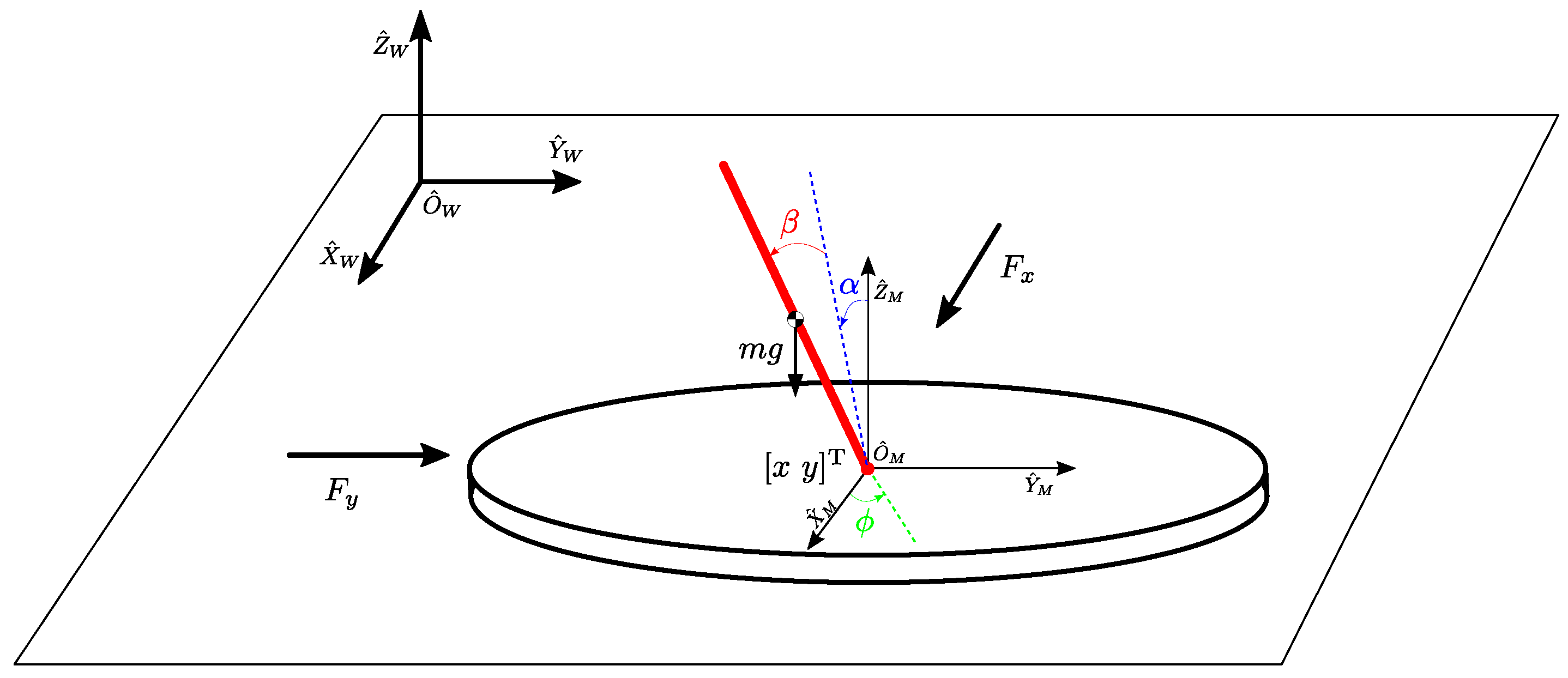
2.3. Model of a Spherical Inverted Pendulum

The mathematical model of a spherical inverted pendulum system is given in this subsection. Figure 4 shows the basic physical symbol description. Assuming that the robot is controlled to have the horizontal movement only. Here the pendulum rod is connected with a universal joint fixed at the robot’s center. Thus, the pendulum rod can freely rotate around the plane axes. The world coordinate system is denoted O ^ W X ^ W Y ^ W Z ^ W , the moving frame is denoted O ^ M X ^ M Y ^ M Z ^ M , and the body frame on the pendulum is o x p y p z p which is attached to the pendulum with the origin located at the robot’s center of mass.
The system variables and parameters are defined as below:
M , m : mass   of   the   mobile   robot   and   the   pendulum ,   respectively . l : length   of   the   pendulum   from   its   center   of   mass   to   the   pivot   point . x , y : the   position   of   the   robot s   center   of   mass   relative   to   the   X ^ W - axis   and     Y ^ W - axis ,   respectively . α , β : the   pendulum s   angular   displacement   around   the X ^ W - axis   and Y ^ W - axis ,     respectively . I p x x , I p y y , I p z z : the   pendulum s   moment   of   inertia   about   the   x p - axis ,   y p - axis ,   and       z p - axis ,   respectively . g : gravitational   acceleration . F x : control   force   applied   to   the   X ^ M - axis . F y : control   force   applied   to   the   Y ^ M - axis .
Again, by the Euler-Lagrange Formula (7) the dynamic equations for the system are derived. For this system, q and Q are chosen as
q = x α y β T ,
Q = F x 0 F y 0 T .
The dynamic equations of the spherical inverted pendulum are obtained as below:
( m + M ) x ¨ + ( m l cos α cos β ) α ¨ + ( m l sin α sin β ) β ¨ + ( m l α ˙ sin α cos β m l β ˙ cos α sin β ) α ˙ + ( m l β ˙ sin α cos β m l α ˙ cos α sin β ) β ˙ = F x ,
( m l cos α cos β ) x ¨ + ( m l 2 cos 2 β + I p y y cos 2 β + I p z z sin 2 β ) α ¨ + ( m l 2 β ˙ sin β cos β I p y y β ˙ sin β cos β + I p z z β ˙ sin β cos β ) α ˙ + ( m l 2 α ˙ sin β cos β I p y y α ˙ sin β cos β + I p z z α ˙ sin β cos β ) β ˙ m g l sin α cos β = 0
( m + M ) y ¨ + ( m l cos β ) β ¨ m l β ˙ 2 sin β = F y ,
( m l sin α sin β ) x ¨ + ( m l cos β ) y ¨ + ( m l 2 + I p x x ) β ¨ + ( m l 2 α ˙ sin β cos β + I p y y α ˙ sin β cos β I p z z α ˙ sin β cos β ) α ˙ m g l cos α sin β = 0 .

2.4. Relationship between Control Forces, Control Torque, and Control Voltages

In the dynamic equations of the rotary or spherical inverted pendulum system, the control input of the system is the planar force or torque generated by the omni-directional wheeled mobile robot. Therefore, the relationship between the control input of the inverted pendulum systems and the acceleration of the omni-directional wheeled mobile robot are given by:
x ¨ = F x M t ,
y ¨ = F y M t ,
ϕ ¨ = τ ϕ I C z z ,
where M t is the mass of the robot with the inverted pendulum and I C z z is the moment of inertia of the robot with the inverted pendulum about the Z ^ M -axis. From (6), (19), (20) and (21), we can obtain the result below:
F x M t F y M t τ ϕ I C z z = A w P ˙ w + B w ( ϕ ) U C .
Finally, in order to obtain the relationship between the control torque, the control force, and the control voltage, using inverse dynamics we obtain
u c = u 1 u 2 u 3 = cos ϕ 3 b 1 ( F x M t a 1 x ˙ ) 3 sin ϕ cos ϕ 6 b 1 ( F x M t a 1 x ˙ ) 3 sin ϕ cos ϕ 6 b 1 ( F x M t a 1 x ˙ ) sin ϕ 3 b 1 ( F y M t a 1 y ˙ ) 3 cos ϕ + sin ϕ 6 b 1 ( F y M t a 1 y ˙ ) 3 cos ϕ + sin ϕ 6 b 1 ( F y M t a 1 y ˙ ) 1 3 b 2 ( τ ϕ I C z z a 2 ϕ ˙ ) 1 3 b 2 ( τ ϕ I C z z a 2 ϕ ˙ ) 1 3 b 2 ( τ ϕ I C z z a 2 ϕ ˙ ) .

3. Using Second-Order Sliding Mode Control to Design the Stabilizing Controllers

The design of the stabilizing controllers for the rotary inverted pendulum and spherical inverted pendulum using second-order sliding mode control is given in this section.

3.1. Controller Design for a Rotary Inverted Pendulum

The design of the stabilizing controller for the rotary inverted pendulum system using second-order sliding mode control is presented in this subsection. From (11) and (12), and by introducing d ϕ 1 which may include the external disturbances and uncertainties of the unmodeled dynamics, the dynamic equations of the rotary inverted pendulum system are rewritten as follows:
β ¨ = 1 Δ ( m l 2 + I P y y I P z z ) ϕ ˙ 2 sin β cos β [ ( m l 2 + I P y y ) sin 2 β + I P z z cos 2 β + m R c 2 + I C z z ] + 2 m l R c ( m l 2 + I P y y I P z z ) ϕ ˙ sin β cos 2 β + m 2 l 2 R c 2 β ˙ sin β cos β + g m l sin β [ ( m l 2 + I P y y ) sin 2 β + I P z z cos 2 β + m R c 2 + I C z z ] m l R c cos β ( τ ϕ + d ϕ 1 ) ,
ϕ ¨ = 1 Δ m l R c ( I p y y I p z z + m l 2 ) ϕ ˙ 2 sin β cos 2 β 2 ϕ ˙ sin β cos β [ m l 2 ( I p x x + I p y y I p z z ) + m 2 l 4 I p x x I p z z + I p x x I p y y ] m l R c ( I p x x + m l 2 ) β ˙ sin β g m 2 l 2 R c sin β cos β + ( m l 2 + I p x x ) ( τ ϕ + d ϕ 1 ) ,
where
Δ = m l 2 + I P y y m l 2 + I P x x sin 2 β m 2 l 2 R c 2 m l 2 I P z z I P x x I P z z cos 2 β + m l 2 + I P x x m R c 2 + I C z z .
In order to obtain the regular form [25], consider the following change of variables
z ϕ = ϕ φ ( β ) ,
where
φ ( β ) = m l 2 + I p x x m l R c ln 1 + tan ( β β 2 2 ) 1 tan ( β β 2 2 )
From (26) and (27), the system Equations (24) and (25) can be rewritten as
z ¨ ϕ = H ( β , ϕ ˙ ) tan β ,
β ¨ = v s ( β , β ˙ , ϕ ˙ , τ ϕ ) + d ϕ ,
where
H ( β , ϕ ˙ ) = g R c + ϕ ˙ 2 m l R c cos β m l 2 + I P y y I P z z cos 2 β + m l 2 + I P x x , v s ( β , β ˙ , ϕ ˙ , τ ϕ ) = 1 Δ [ ( I P z z m l 2 I P y y ) ϕ ˙ 2 sin β cos β + g m l sin β ] [ ( m l 2 + I P y y ) sin 2 β + I P z z cos 2 β + m R c 2 + I C z z ]
+ m l R c cos β [ 2 ( m l 2 + I P y y I P z z ) ϕ ˙ sin β cos β + β ˙ m l R c sin β τ ϕ ] .
d ϕ = m l R c cos β Δ d ϕ 1
Select the following coupled sliding variables [22]:
s ϕ = k ( z ˙ ϕ + a z ϕ ) + ( β ˙ + b β )
where k, a, and b are constant parameters. For ensuring semi-globally asymptotical stability of the closed-loop system over the upper-half plane, a sufficient condition for determining k, a, and b will be derived in the sequel. After differentiating s ϕ , we have
s ˙ ϕ = k ( z ¨ ϕ + a z ˙ ϕ ) + β ¨ + b β ˙ = k [ H ( β , ϕ ˙ ) tan β + a z ˙ ϕ ] + v s ( β , β ˙ , ϕ ˙ , τ ϕ ) + b β ˙ + d ϕ .
From (34), the system Equations (28) and (29) have a relative degree of one with respect to s ϕ . The following control inputs is defined
v = v s ( β , β ˙ , ϕ ˙ , τ ϕ ) + k [ H ( β , ϕ ˙ ) tan β + a z ˙ ϕ ] + b β ˙ .
then from (34) and (35), we obtain
s ˙ ϕ = v + d ϕ .
The super-twisting algorithm [16,26,27] is one of the most widely used second-order sliding mode controllers that is designed for systems of relative degree one. Assuming that the global bound of the unknown disturbance d ϕ is give by
d ϕ δ s ϕ 1 2
for some constant δ > 0 . The super-twisting sliding mode controller is given by
v = λ s ϕ 1 2 sgn ( s ϕ ) + v 1 ,
v ˙ 1 = W sgn ( s ϕ ) ,
where the usual signum function is represented by the function sgn ( · ) and, λ and W are constant gains satisfying the following conditions:
λ > 2 δ , W > λ 5 δ λ + 4 δ 2 2 ( λ 2 δ ) .
It can be shown that in the presence of disturbances, the control law (38) and (39) guarantees the convergence of the closed-loop state trajectory onto the sliding manifold s ϕ = 0 and s ˙ ϕ = 0 in a finite time. Note that unlike the conventional sliding mode control, the super-twisting algorithm given in (38) and (39) is a continuous control that can attenuate the chattering problems effectively. Finally, according to (35) and (31), the control torque is given by
τ ϕ = 1 m l R c cos β { [ v k H ( β , ϕ ˙ ) tan β k a z ˙ ϕ b β ˙ ] · Δ + ϕ ˙ 2 sin β cos β [ ( I p z z m l 2 I p y y ) ( m R c 2 + m l 2 sin 2 β + I p y y sin 2 β + I p z z cos 2 β ) m l 2 I c z z ] g m l sin β ( m l 2 sin 2 β + I p y y sin 2 β + I p z z cos 2 β + m R c 2 + I C z z ) m 2 l 2 R c 2 β ˙ sin β cos β 2 m l R c ( m l 2 + I p y y I p z z ) ϕ ˙ sin β cos 2 β } .
For translational motion, a controller needs to be designed to keep the position of the mobile robot without any translational movement. For this purpose, the translational motion of the mobile robot in the X and Y axes is designed by the PD controller as follows:
F x = K x 1 x ˙ K x 2 x , F y = K y 1 y ˙ K y 2 y .
where K x 1 , K x 2 , K y 1 and K y 2 are positive constants. Finally, substituting the control torque (41) and control forces (42) into (23), the corresponding control voltages for the three motors can be obtained.

Stability Analysis of Zero Dynamics

Closed-loop stability analysis the rotary inverted pendulum system using the proposed control scheme is presented in this subsection. From (34), the equivalent control [17] for s ˙ ϕ = 0 is given by
u e q = k [ H ( β , ϕ ˙ ) tan β + a z ˙ ϕ ] b β ˙ d ϕ .
Substituting (43) into (29), we obtain
β ¨ = b β ˙ k a z ˙ ϕ k [ H ( β , ϕ ˙ ) tan β ] .
Since the sliding mode s ϕ ( t ) = 0 is established for all t t 0 , it gives
z ˙ ϕ + a z ϕ = k 1 ( β ˙ + b β ) .
From (45), we have
z ϕ ( t ) = z ϕ ( t 0 ) e a ( t t 0 ) k 1 t 0 t [ β ˙ ( τ ) + b β ( τ ) ] e a ( t τ ) d τ , = z ϕ ( t 0 ) e a ( t t 0 ) k 1 [ β ( τ ) e a ( t τ ) ] t 0 t + k 1 t 0 t β ( τ ) d d τ e a ( t τ ) d τ k 1 b t 0 t β ( τ ) e a ( t τ ) d τ , = [ z ϕ ( t 0 ) + k 1 β ( t 0 ) ] e a ( t t 0 ) k 1 β ( t ) + k 1 ( a b ) t 0 t β ( τ ) e a ( t τ ) d τ .
From (45) and (46), it gives that
z ˙ ϕ = a z ϕ k 1 ( β ˙ + b β ) , = a [ z ϕ ( t 0 ) + k 1 β ( t 0 ) ] e a ( t t 0 ) k 1 β + k 1 ( a b ) t 0 t β ( τ ) e a ( t τ ) d τ k 1 ( β ˙ + b β ) .
Substituting (47) into (44), it follows that
β ¨ = b β ˙ k a { a { [ z ϕ ( t 0 ) + k 1 β ( t 0 ) ] e a ( t t 0 ) k 1 β + k 1 ( a b ) t 0 t β ( τ ) e a ( t τ ) d τ } k 1 ( β ˙ + b β ) } k [ H ( β , ϕ ˙ ) tan β ] , = ( a b ) β ˙ + ( a b a 2 ) β + a 2 ( a b ) t 0 t β ( τ ) e a ( t τ ) d τ k H ( β , ϕ ˙ ) tan β + k a 2 [ z ϕ ( t 0 ) + k 1 β ( t 0 ) ] e a ( t t 0 ) .
Denote
w ( t ) = t 0 t β ( τ ) e a ( t τ ) d τ .
By taking time derivative of w ( t ) and let w ( t 0 ) = 0 , we have
w ˙ ( t ) = d d t t 0 t β ( τ ) e a ( t τ ) d τ , = β ( τ ) e a ( t τ ) τ = t + t 0 t t [ e a ( t τ ) ] β ( τ ) d τ , = β ( t ) + t 0 t a e a ( t τ ) β ( τ ) d τ , = β ( t ) a w ( t ) .
Thus form (48)–(50), it follows that the zero dynamics of the system constrained to the manifold of s ϕ = 0 and s ˙ ϕ = 0 are given by
β ¨ = ( a b ) β ˙ + ( a b a 2 ) β + a 2 ( a b ) w k H ( β , ϕ ˙ ) tan β + k a 2 [ z ϕ ( t 0 ) + k 1 β ( t 0 ) ] e a ( t t 0 ) , w ˙ = β a w .
During the sliding mode, the system dynamics become insensitive to the matched disturbances, and the effects of the disturbance are completely eliminated, as seen in (51).
To show that the zero dynamics (51) over the upper-half plane is semi-globally asymptotically stable, the stability of the following system is first investigated:
β ¨ = ( a b ) β ˙ + ( a b a 2 ) β + a 2 ( a b ) w k H ( β , ϕ ˙ ) tan β , w ˙ = β a w .
Note that the unforced system (52) is the zero dynamics (51) in the absence of external excitation. Also note that in (52), the nonlinear term is
H ( β , ϕ ˙ ) tan β = g R c + ϕ ˙ 2 m l R c cos β m l 2 + I P y y I P z z cos 2 β + m l 2 + I P x x tan β
Define the state vector as
x z = x 1 x 2 x 3 = β β ˙ w .
The configuration of the Lur’e system [28] can be used to formulate the system (52) as follows:
x ˙ z = 0 1 0 ( a b a 2 ) ( a b ) a 2 ( a b ) 1 0 a x z + 0 k 0 u z ,
y z = [ 1 0 0 ] x z ,
u z = ψ ( t , y z ) = H ( β , ϕ ˙ ) tan β .
Note that in (57) ψ is a time varying nonlinearity, whose time variation depends on ϕ ˙ . From (41), the system has a singularity at β = ± π 2 . Therefore, the domain of the open upper-half plane β π 2 ε is considered, where ε is sufficiently small and 0 < ε π 2 . For β π 2 ε , the nonlinearity ψ ( t , y z ) lies in the sector of [ g 1 , K 2 ] with g 1 K 2 < and g 1 = g R c . Denote G 0 ( s ) to be the transfer function from u z to y z . Here
G 0 ( s ) = k ( s + a ) s 2 ( s + b ) .
The following lemma is based on the circular criterion [28].
Lemma 1.
The system (55)–(57) is asymptotically stable for x z x z R 3 x 1 π 2 ε , if 1 + K 2 G 0 ( s ) 1 + g 1 G 0 ( s ) is strictly positive real.
Remark 1.
Let
G 1 ( s ) = 1 + K 2 G 0 ( s ) 1 + g 1 G 0 ( s ) , = s 2 ( s + b ) + K 2 k ( s + a ) s 2 ( s + b ) + g 1 k ( s + a ) .
A sufficient condition of a, b, and k for having G 1 ( s ) be strictly positive real is given below. For transfer function G 1 ( s ) to be strictly positive real, G 1 ( s ) is analytic in R e [ s ] 0 and R e [ G 1 ( j ω ) ] > 0 for all ω R . Based on the Routh-Hurwitz criterion [29], we have
k > 0 , b > a > 0 ,
to guarantee G 1 ( s ) to be Hurwitz stable, i.e., analytic in R e [ s ] 0 . Now consider
R e [ G 1 ( j ω ) ] = R e ( b ω 2 + K 2 k a ) + j ω ( ω 2 + K 2 k ) ( b ω 2 + g 1 k a ) + j ω ( ω 2 + g 1 k ) , = ( b ω 2 + K 2 k a ) ( b ω 2 + g 1 k a ) + ω 2 ( ω 2 + K 2 k ) ( ω 2 + g 1 k ) ( b ω 2 + g 1 k a ) 2 + ω 2 ( ω 2 + g 1 k ) 2 .
Denote the denominator of (61) to be
Δ G 1 ( ω ) = ( b ω 2 + g 1 k a ) 2 + ω 2 ( ω 2 + g 1 k ) 2 .
Then, we have
R e [ G 1 ( j ω ) ] = ω 6 + [ b 2 k ( K 2 + g 1 ) ] ω 4 + [ K 2 g 1 k 2 b k a ( K 2 + g 1 ) ] ω 2 + K 2 g 1 k 2 a 2 Δ G 1 ( ω ) .
If
b 2 > k ( K 2 + g 1 ) , K 2 g 1 k 2 > b k a ( K 2 + g 1 ) ,
it gives that R e [ G 1 ( j ω ) ] > 0 for all ω R . By simply choosing
k = K 2 + g 1 , b > K 2 + g 1 , a b < K 2 g 1 ,
it follows that inequalities of (64) are satisfied such that R e [ G 1 ( j ω ) ] > 0 for all ω R . From (60) and (65), it follows that G 1 ( s ) is strictly positive real if
b > a > 0 , k = K 2 + g 1 , b > K 2 + g 1 , a b < K 2 g 1 ,
The condition (66) shows that for given K 2 > g 1 > 0 there always exist a, b, and k such that G 1 ( s ) is strictly positive real.
Consider the following system
x ˙ z = f z ( t , x z ) + A e a 1 ( t t 0 ) ,
where x z R n , f : R + × R n R n is a sufficiently smooth vector field and f z ( t , 0 ) = 0 for t > t 0 0 , A is an n × 1 matrix, a 1 > 0 and t > t 0 0 .
Lemma 2.
Consider the system as defined in (67) and assume a continuously differentiable function V 0 ( t , x z ) : R + × R n R exists which satisfy
c 1 x z 2 V 0 ( t , x z ) c 2 x z 2 , V 0 t + V 0 x z f z ( t , x z ) c 3 x z 2 , V 0 x z A c 4 x z ,
where c 1 , c 2 , c 3 , and c 4 are some positive constants. Then, the globally exponential stability at the origin of the system (67) is obtained.
Proof. 
Consider the following first-order linear differential equation
ξ ˙ ( t ) = a 1 ξ ( t ) , t t 0 0 ,
Then the solution of (69) is
ξ ( t ) = c 0 e a 1 ( t t 0 ) , t t 0 0 ,
where c 0 = ξ ( t 0 ) 0 is a constant. The system (67) can be written using the augmented state ξ as
x ˙ z = f ( t , x z ) + A c 0 ξ , ξ ˙ = a 1 ξ .
Now, the following Lyapunov candidate functions is considered
V ( t , x z , ξ ) = V 0 ( t , x z ) + 1 2 η ξ 2 ,
where η is a positive constant. The derivative of V along the trajectory of (71) is given by
V ˙ ( t , x z , ξ ) = V 0 t + V 0 x z [ f z ( t , x z ) + A c 0 ξ ] a 1 η ξ 2 , = V 0 t + V 0 x z f z ( t , x z ) + 1 c 0 V 0 x z A ξ a 1 η ξ 2 , c 3 x z 2 + c 4 c 0 x z · ξ a 1 η ξ 2 , = c 3 x z 1 2 c 4 c 3 c 0 ξ 2 a 1 η 1 4 c 4 2 c 3 c 0 2 ξ 2 .
By denoting
x z a = x z ξ .
and choosing η such that
a 1 η 1 4 c 4 2 c 3 c 0 2 > 0 ,
we have
V ˙ ( t , x z , ξ ) c 5 x z a 2 c 6 V ( t , x z , ξ )
where c 5 and c 6 are a positive constants. It concludes that the origin of the system (67) is globally exponentially stable. □
Now, we are ready to state the stability of the zero dynamics of (51).
Theorem 1.
(stability of zero dynamics):The transfer function G 1 ( s ) = s 2 ( s + b ) + K 2 k ( s + a ) s 2 ( s + b ) + g 1 k ( s + a ) is strictly positive real with the appropriately chosen parameters of a, b, and k. Then, the semi-global asymptotic stability can be obtained over the upper-half plane for the equilibrium point of the zero dynamics (51).
Proof. 
The zero dynamics (51) can be written as
x ˙ z = f z ( t , x z ) + A e a ( t t 0 ) ,
with
x z = x 1 x 2 x 3 = β β ˙ w ,
f z ( t , x z ) = x 2 ( a b ) x 2 + ( a b a 2 ) x 1 + a 2 ( a b ) w k H ( x 1 , ϕ ˙ ) tan x 1 x 1 a x 3 ,
A = 0 k a 2 [ z ϕ ( t 0 ) + k 1 β ( t 0 ) ] 0 .
According to Lemma 1 and Kalman-Yakubovich-Popov lemma [30], there is a Lyapunov candidate function V ( x z ) = 1 2 x z T P x z with positive definite matrix P when G 1 ( s ) is strictly positive real. Along the trajectories of the unforced system x ˙ z = f z ( t , x z ) , the time derivative of V ( x z ) is given by
V ˙ ( x z ) = V x z f z k 3 x z T P x z ,
where k 3 > 0 , and for some ε > 0 , x z Ω = { x z R 3 x 1 π 2 ε } . Now, for the forced system (77), with
λ min ( P ) x z 2 V ( x z ) λ max ( P ) x z 2 ,
V x z f z k 3 x z T P x z ,
V x z A k 4 x z ,
where λ min ( P ) and λ max ( P ) denote the minimum and maximum eigenvalue of P, respectively, and k 4 > 0 . It follows immediately from Lemma 2 that the equilibrium point of the zero dynamics (51) is semi-globally asymptotically stable over Ω = { x R 3 x 1 π 2 ε } . □
Theorem 2.
(stability of the closed-loop system):The sliding variables (33) and the controller defined by (38), (39), and (41) ensure that the equilibrium point of the rotary inverted pendulum system is semi-globally asymptotically stable in the upper-half plane.
Proof. 
It can be known from Theorem 1 that the semi-globally asymptotic stability can be obtained over the upper-half plane for the zero dynamics of the closed-loop system. It implies that β 0 , β ˙ 0 as t . Therefore, on the sliding manifold s ϕ = 0 , from (33), we have z ˙ ϕ + a z ϕ 0 as t . Because a > 0 , it gives that z ϕ 0 , z ˙ ϕ 0 as t . From β 0 , β ˙ 0 , z ϕ 0 , z ˙ ϕ 0 , and (26), it follows that ϕ 0 , ϕ ˙ 0 as t . This concludes that on the sliding manifold, the closed-loop system is semi-globally asymptotically stable over Ω . □

3.2. Controller Design of Spherical Inverted Pendulum

The design of the stabilizing controller for the spherical inverted pendulum system using second-order sliding mode control is presented in this subsection. Clearly, the dynamics given in (15)–(18) are highly nonlinear and dynamically coupled. The system model simplification is required because the system model is too complex to be used directly in the control design. By symmetry of the system, the spherical inverted pendulum system can be viewed as a two-dimensional extension of the traditional cart-pole inverted pendulum system [31]. The angular displacements α and β are small for balance control, so cross-coupling is neglectable. The system can be simplified and decoupled into two independently cart-pole inverted pendulum systems as follows
( m + M ) x ¨ + ( m l cos α ) α ¨ ( m l α ˙ sin α ) α ˙ = F x ,
( m l cos α ) x ¨ + ( m l 2 + I P y y ) α ¨ m g l sin α = 0 ,
( m + M ) y ¨ + ( m l cos β ) β ¨ ( m l β ˙ sin β ) β ˙ = F y ,
( m l cos β ) y ¨ + ( m l 2 + I P x x ) β ¨ m g l sin β = 0 ,
From (85)–(88), we can see that two cart-pole inverted pendulum systems in the X-axis and Y-axes are identical. Next, only the controller design of the cart-pole inverted pendulum system in the X axis is addressed. By introducing a disturbance or uncertainty d x 1 which may include external disturbance, parametric perturbation, and unmodeled dynamics, the dynamic Equations (85) and (86) is rewritten as follows
x ¨ = ( m l 2 + I p y y ) ( m l α ˙ 2 sin α ) m 2 l 2 g sin α cos α m 2 l 2 + M m l 2 + ( m + M ) I P y y m 2 l 2 cos 2 α + m l 2 + I p y y m 2 l 2 + M m l 2 + ( m + M ) I P y y m 2 l 2 cos 2 α ( F x + d x 1 ) ,
α ¨ = m 2 l 2 α ˙ 2 sin α cos α + ( m + M ) m g l sin α m 2 l 2 + M m l 2 + ( m + M ) I P y y m 2 l 2 cos 2 α + m l cos α m 2 l 2 + M m l 2 + ( m + M ) I P y y m 2 l 2 cos 2 α ( F x + d x 1 ) .
To obtain the regular form for the system of (89) and (90), the following change of variables is used
z x = x φ ( α ) ,
where
φ ( α ) = m l 2 + I p y y m l ln 1 + tan ( α α 2 2 ) 1 tan ( α α 2 2 )
Then the regular form is given by
z ¨ x = H ( α , α ˙ ) tan α ,
α ¨ = v s ( α , α ˙ , F x ) + d x ,
where
H ( α , α ˙ ) = g + m l 2 + I p y y m l cos α α ˙ 2 ,
v s ( α , α ˙ , F x ) = m 2 l 2 α ˙ 2 sin α cos α + ( m + M ) m g l sin α ( m + M ) ( m l 2 + I p y y ) m 2 l 2 cos 2 α + m l cos α ( m + M ) ( m l 2 + I p y y ) m 2 l 2 cos 2 α F x ,
d x = m l cos α ( m + M ) ( m l 2 + I p y y ) m 2 l 2 cos 2 α d x 1 .
The following coupled sliding variable is chosen:
s x = k x ( z ˙ x + a x z x ) + ( α ˙ + b x α )
where k x , a x , and b x are constant parameters. By referring to the condition of (68), the appropriate k x , a x , and b x can be selected to guarantee that the closed-loop system is asymptotically stable. Differentiating s x yields
s ˙ x = k x ( z ¨ x + a x z ˙ x ) + α ¨ + b x α ˙ = k x [ H ( α ˙ , α ˙ ) tan α + a x z ˙ x ] + v s ( α , α ˙ , F x ) + b x α ˙ + d x .
System Equations (93) and (94) whose relative degree is one relative to s x . Define the following control input
v = v s ( α , α ˙ , F x ) + k x [ H ( α , α ˙ ) tan α + a x z ˙ x ] + b x α ˙ .
then obtain
s ˙ x = v + d x .
Again, the following super-twisting sliding mode controller is used
v = λ x s x 1 2 sgn ( s x ) + v 1 ,
v ˙ 1 = W x sgn ( s x ) ,
where λ x and W x are positive constant gains. Finally, from (100) and (96), the control force is given by
F x = 1 m l cos α { [ v k x H ( α , α ˙ ) tan α k x a x z ˙ x b x α ˙ ] [ ( m + M ) ( m l 2 + I p y y ) m 2 l 2 cos 2 α ] + m 2 l 2 α ˙ 2 sin α cos α ( m + M ) m g l sin α } .
In the same way, the cart-pole inverted pendulum system in the Y-axis also uses the same design method to obtain the control force F y . Stability analysis of the closed-loop system is omitted since it follows along the same limes as the proofs of Theorem 1 and Theorem 2.
It is supposed that the controlled omn-idirectional wheeled mobile robot only has planar motion without any rotational movement in the balance control of the spherical inverted pendulum system. Therefore, in order to keep the mobile robot not rotating during the balancing process, a controller needs to be designed for the rotational motion. To this end, a proportional-derivative (PD) controller for the rotational motion control of the mobile robots is designed as follows:
τ ϕ = K ϕ 1 ϕ ˙ K ϕ 2 ϕ ,
where K ϕ 1 and K ϕ 2 are positive constants. In this way, the mobile robot is controlled to have the rotation angle ϕ to be zero. Finally, by substituting the plane control forces F x and F y and the control torque τ ϕ into (23), the control voltages of the motors can be obtained.

4. Explanation of the Experimental Device

An experimental setup which can be configurated as a rotary inverted pendulum or a spherical inverted pendulum on an omni-directional wheeled mobile robot was built as shown in Figure 5. A two-axis gimbal mechanism is used to enable the pendulum rod to rotate in pitch and yaw direction for the spherical inverted pendulum. One of the rotation axes can be fixed for the rotatory inverted pendulum. This gimbal mechanism can be mounted on the center or off-center of the platform of the mobile robot. Optical encoders measure the angular displacement of the pendulum with a resolution of 2000 pulses/rev. The robot is driven by brushed dc motors with optical encoders with a resolution of 500 pulses/rev. The designed control laws are implemented on an in-house embedded system based on a digital signal processor. There are two quadrature decoders and a pulse width modulation (PWM) generator for the digital signal processing board. The PWM driver circuits are used to drive each brushed dc motor. The sampling rate of the system is set to 1 kHz. The quadrature signal is generated by the optical encoder measuring the angular displacement of the pendulum, and then this signal inputs to the quadrature decoder on the digital signal processing board. The optical encoder mounted on the motor generates quadrature signals, which are then input to a quadrature decoder circuit implemented on a Field Programmable Gate Array (FPGA) board. The difference in consecutive encoder counts read per unit time is used to estimate the angular velocity of the pendulum and wheels. For noise caused by this differential action, a low-pass filter is used to attenuate it. A dead reckoning algorithm is used to determine the position and orientation of the mobile robot.

5. Simulation and Experimental Results

The simulation studies are conducted using the Simulink software to verified designed control schemes. The designed sliding mode control laws are implemented and tested on the experimental setup show in Figure 5. Based on the linearized system models, the classical LQR (Linear Quadratic Regulator) controllers are designed and applied to the systems for performance comparison. Conventional sliding mode controllers based on our previous work [15] are also designed and tested for performance comparison.

5.1. Simulation Results of Rotary Inverted Pendulum

The simulation results for the rotary inverted pendulum system are shown in Figure 6, Figure 7 and Figure 8. From the simulation results, the LQR controller, conventional sliding mode controller, and second-order sliding mode controller all can stabilize the rotary inverted pendulum system. Moreover, from Figure 6, the system with the LQR controller and conventional sliding mode controller have more significant overshoots in the angular displacements of the pendulum and robot. Figure 7 and Figure 8 shows that the system with LQR controller and conventional sliding mode controller have significant position deviation of the robot. From the simulation results, it can be seen that the system with second-order sliding mode control has better performance, in terms of less overshoot, faster convergence in the pendulum angle, and less position deviation of the robot. Table 1 summarizes the simulation results of the maximum deviations of the pendulum’s angle, the robot’s rotation angle, and robot’s position. A sinusoidal disturbance with a frequency of 10 rad/s is added to the control torque in the simulation to show the robustness of the sliding mode control schemes. Figure 9 shows that all three controllers can balance the rotary inverted pendulum even with the disturbance, but both sliding mode controllers have a less significant steady-state oscillation in the pedulum’s angle and the robot’s rotation angle than the LQR controller. To access the control system’s robustness to the pendulum’s initial deviation, a large initial deviation from its upright position is considered in the simulation. Figure 10 shows that the proposed second-order sliding mode controller allows an initial deviation of 40 of the pendulum from its upright position, whereas for the conventional sliding mode controller and LQR controller, the system is no longer stabilizable and the response becomes divergent.

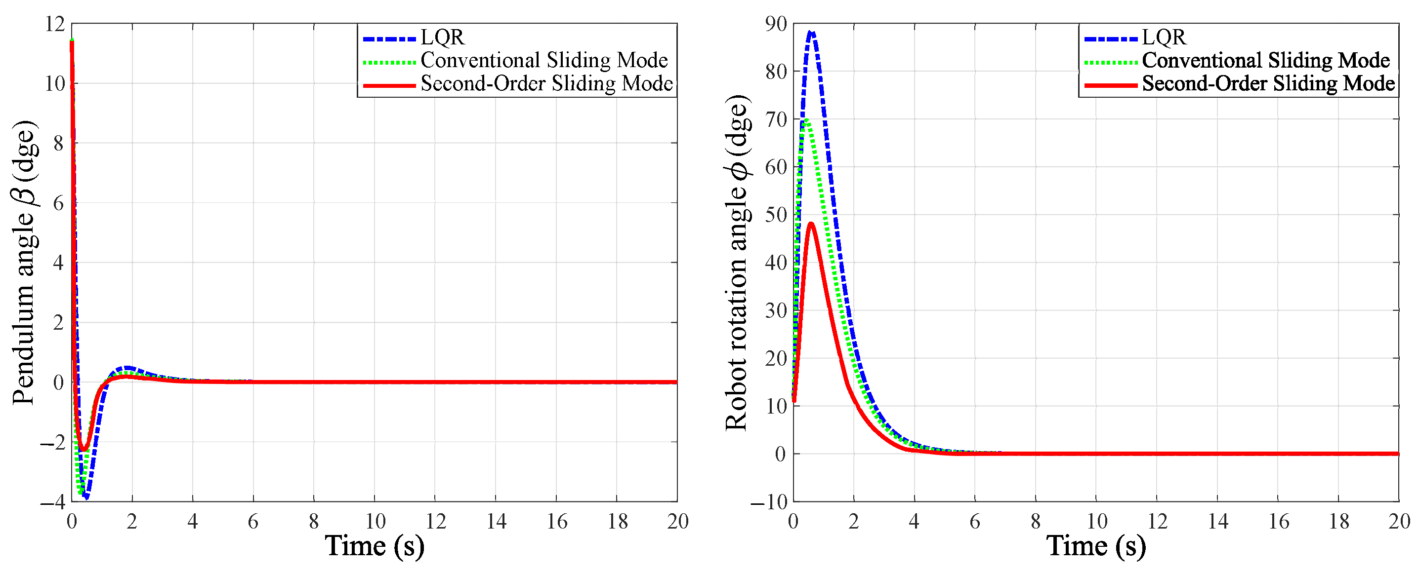
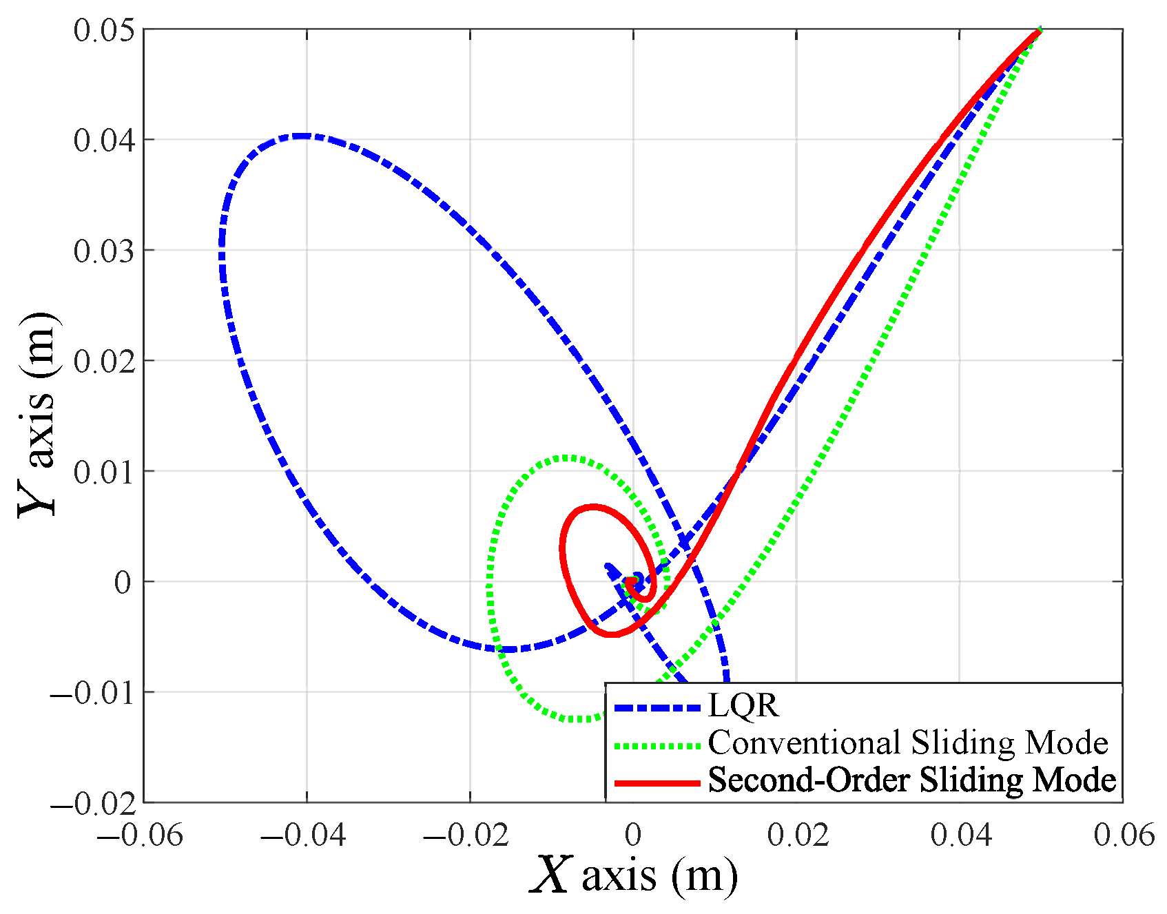
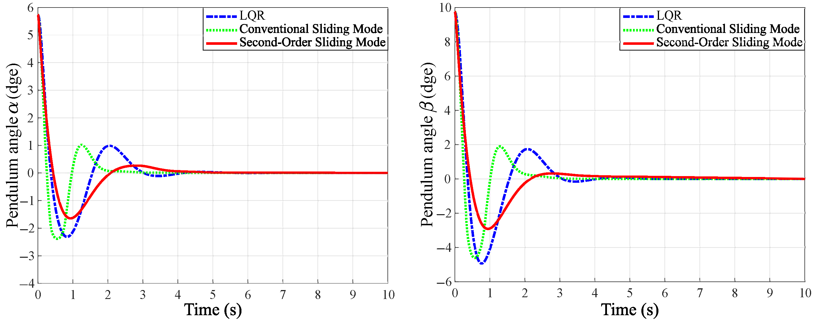
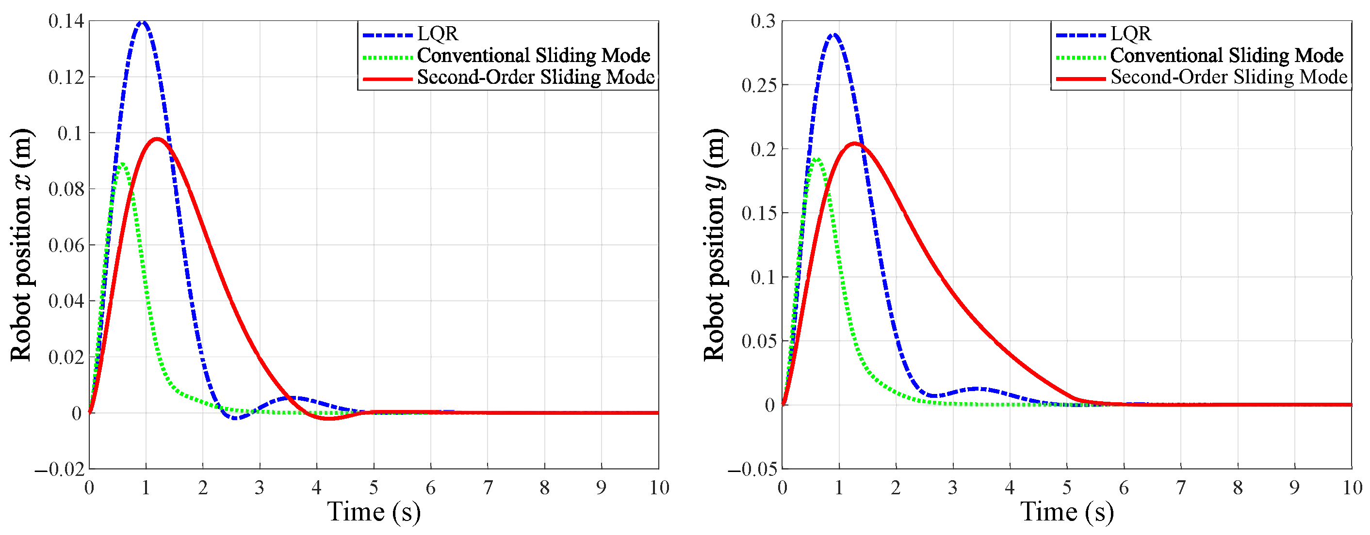
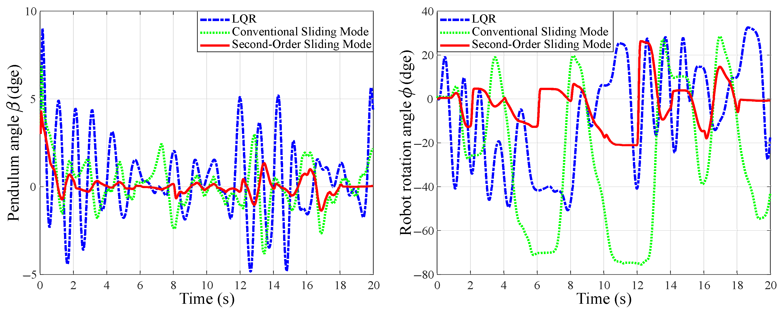
5.2. Simulation Results of Spherical Inverted Pendulum

For the spherical inverted pendulum system, the simulation results of the pendulum’s angular displacement response, the robot’s position response, the robot’s rotation angle response, and the robot’s trajectory are shown in Figure 11, Figure 12 and Figure 13, respectively. The simulation results show that the spherical inverted pendulum system is stabilized by all the designed control laws. Moreover, from Figure 11, the system with LQR controller and conventional sliding mode controller have more significant overshoots in the angular displacements of the pendulum. Figure 12 and Figure 13a show that the system with the LQR controller also has a significant position deviation of the robot. Figure 13b shows that the second-order sliding mode controller has less overshoot and faster convergence in the rotation angle of the robot. From the simulation results, it can be seen that the system with second-order sliding mode control has better performance in terms of less overshoots and faster convergence in the angular displacements of the pendulum and rotation angle of the robot. Table 2 summarizes the simulation results of the maximum deviations of the pendulum’s angles, the robot’s rotation angle, and the robot’s positions. Sinusoidal disturbances with a frequency of 10 rad/s are added to the control forces in the simulation to show the robustness of the sliding mode control schemes. Figure 14 and Figure 15 show that all three controllers can balance the rotary inverted pendulum even with the disturbances, but both sliding mode controllers have a less significant steady-state oscillation in the pendulum’s angular displacements and robot’s positions than the LQR controller. Figure 16 shows that the proposed second-order sliding mode controller allows an initial deviation of 30 of the pendulum from its upright position, whereas for the conventional sliding mode controller and LQR controller, the system is no longer stabilizable and the response becomes divergent.

5.3. Experimental Results of Rotary Inverted Pendulum

For the rotary inverted pendulum system, the experimental results are shown in Figure 17, Figure 18 and Figure 19. From the experimental results, the LQR controller, conventional sliding mode controller, and second-order sliding mode controller all can stabilize the rotary inverted pendulum system. In Figure 17, for second-order sliding mode control, in the steady-state the pendulum oscillates slightly within a range of ± 2 in the β angle, and the rotation angle of the robot oscillates within a range of 20 to + 30 in the angle of ϕ . For LQR control, in the steady-state the pendulum oscillates slightly within a range of ± 5 in the β angle, and the rotation angle of the robot oscillates within a range of 40 to + 30 in the angle of ϕ . For conventional sliding mode control, in the steady-state the pendulum oscillates slightly within a range of ± 3 in the β angle, and the rotation angle of the robot oscillates within a range of 75 to + 30 in the angle of ϕ . It show that second-order sliding mode control has better performance in terms of less steady-state variations in angular displacement of the pendulum and rotation angle of the robot. Figure 18 and Figure 19 show that the LQR-controlled system has apparent robot position deviation. Table 3 summarizes the experimental results of the steady-state oscillating range of the pendulum’s angle, the steady-state oscillating range of the robot’s rotation angle, and the maximum deviation of the robot’s positions.

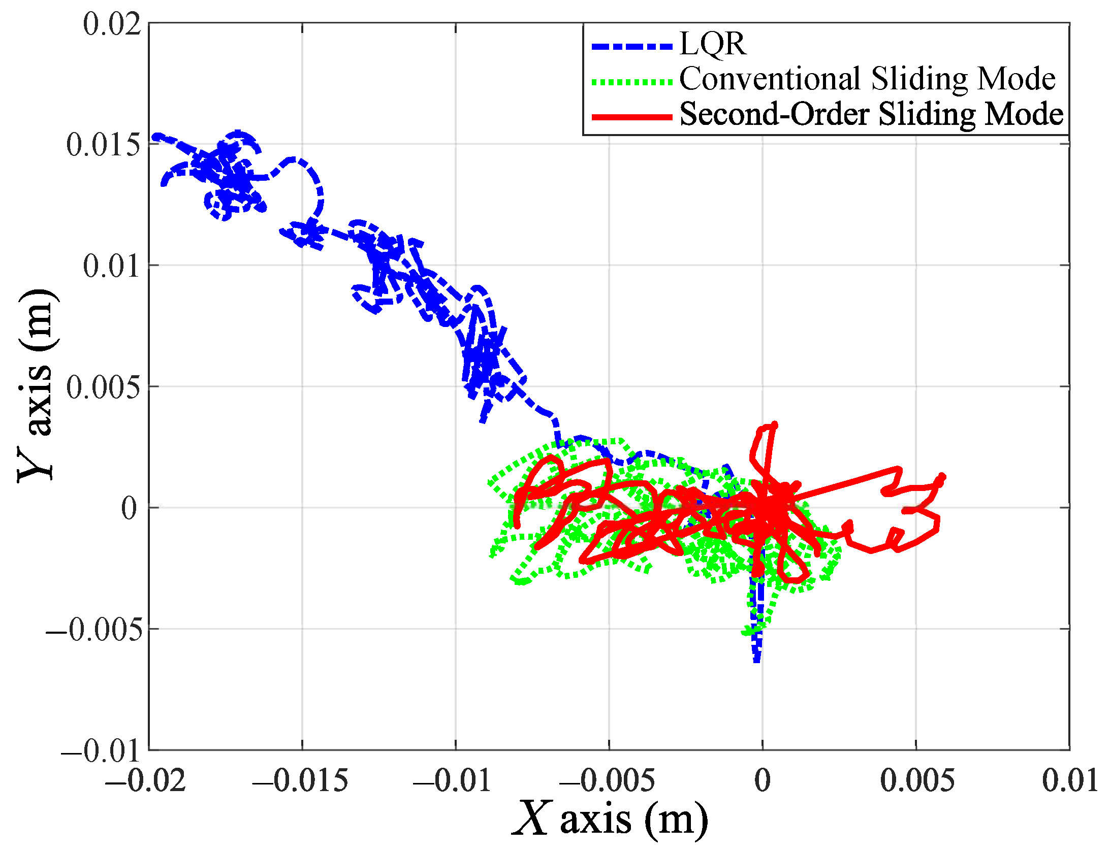
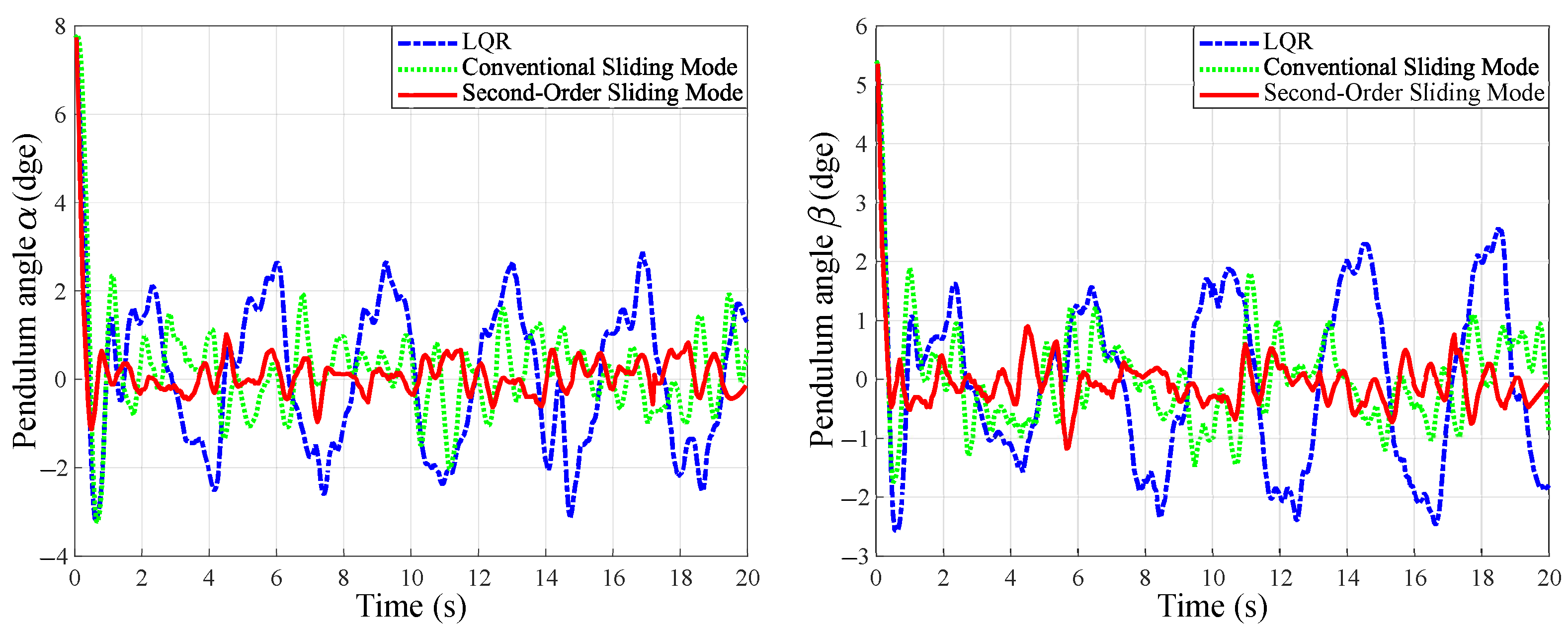
5.4. Experimental Results of Spherical Inverted Pendulum

For the spherical inverted pendulum system, the experimental results of the pendulum’s angular displacement response, the robot’s position response, the robot’s rotation angle response, and the robot’s trajectory are shown in Figure 20, Figure 21 and Figure 22, respectively. The experimental results show that the spherical inverted pendulum system can be stabilized by all the designed control laws. It can be seen from Figure 20 that for the second-order sliding mode control in the steady-state, the pendulum swings slightly on α in the range of ± 1 and on β in the range of ± 1 when the pendulum is in the upright position. For LQR control in the steady-state, the pendulum swings slightly on α in the range of ± 3 and on β in the range of ± 2 . 5 when the pendulum is in the upright position. For conventional sliding mode control in the steady-state, the pendulum swings slightly on α in the range of ± 2 and on β in the range of ± 2 when the pendulum is in the upright position. From Figure 21 and Figure 22a, LQR control has significant position deviation of the robot, and second-order sliding mode control has less position deviation of the robot. Figure 22b shows that the rotation angle ϕ of the robot has a slight variation around 0 in these control strategies, and second-order sliding mode control has fewer variations. Overall it shows that second-order sliding control gives better performance over LQR control and conventional sliding mode control. Table 4 summarizes the experimental results of the steady-state oscillating range of the pendulum’s angles, the steady-state oscillating range of robot’s rotation angle, and the maximum deviation of the robot’s positions.

6. Concluding Remarks

This paper used an omni-directional wheeled mobile robot to balance the configurable inverted pendulum system. The stabilizing control laws of the systems were designed, realized, and experimentally tested. The system’s mathematical models were derived for the control design. The controllers were designed based on the second-order sliding mode control. The results showed that the proposed control law guarantees the closed-loop system to be semi-globally asymptotically stable in the upper-half plane. The experimental setup was built, and the controllers were realized. The designed control system demonstrated to be effective in simulation and experimental results. In the simulation studies, for the rotary pendulum system without any uncertainty and disturbance, the second-order sliding mode control yields a smaller pendulum angle deviation, a smaller robot rotation angle deviation, and a smaller robot position deviation than other controllers. For the system with the sinusoidal matched disturbance, the simulation shows that the second-order sliding-mode controller also has a less significant steady-state oscillation in the pendulum’s angle and a less significant steady-state oscillation in the robot rotation angle than other controllers. Furthermore, only the second-order sliding mode controller can stabilize the system with an initial deviation of 40 of the pendulum from its upright position. For the spherical pendulum without any uncertainty and disturbance in the simulation studies, the second-order sliding mode control also yields smaller pendulum angle deviations, a smaller robot rotation angle, and a smaller robot position deviation than other controllers. For the system with the sinusoidal matched disturbance, the simulation shows that the second-order sliding mode controller also has a less significant steady-state oscillation in the pendulum’s angle and a less significant robot position oscillation than other controllers. Furthermore, only a second-order sliding mode controller can stabilize the system with an initial deviation of 30 of the pendulum from its upright position. It is shown in the experimental results that the second-order sliding mode control is more effective than the LQR control based on the linearized system model and the conventional sliding mode control of our previous work.

Author Contributions

Methodology, S.-T.K. and M.-T.H.; Software, S.-T.K.; Supervision, M.-T.H.; Validation, S.-T.K.; Writing—original draft, S.-T.K.; Writing—review & editing, S.-T.K. and M.-T.H. All authors have read and agreed to the published version of the manuscript.

Funding

This research received no external funding.

Institutional Review Board Statement

No applicable.

Informed Consent Statement

No applicable.

Data Availability Statement

Data collected through research presented in the paper are available on request from the corresponding author.

Conflicts of Interest

The authors declare no conflict of interest.

References

  1. Kajita, S.; Benallegue, M.; Cisneros, R.; Sakaguchi, T.; Nakaoka, S.; Morisawa, M.; Kaneko, K.; Kanehiro, F. Biped walking pattern generation based on spatially quantized dynamics. In Proceedings of the 2017 IEEE-RAS 17th International Conference on Humanoid Robotics (Humanoids), Birmingham, UK, 15–17 November 2017; IEEE: Piscataway, NJ, USA, 2017. [Google Scholar] [CrossRef]
  2. Babazadeh, R.; Khiabani, A.G.; Azmi, H. Optimal control of Segway personal transporter. In Proceedings of the 2016 4th International Conference on Control, Instrumentation, and Automation (ICCIA), Qazvin, Iran, 27–28 January 2016; IEEE: Piscataway, NJ, USA, 2016. [Google Scholar] [CrossRef]
  3. Han, S.I.; Lee, J.M. Balancing and Velocity Control of a Unicycle Robot Based on the Dynamic Model. IEEE Trans. Ind. Electron. 2015, 62, 405–413. [Google Scholar] [CrossRef]
  4. Bakarac, P.; Kaluz, M.; Cirka, L. Design and development of a low-cost inverted pendulum for control education. In Proceedings of the 2017 21st International Conference on Process Control (PC), Strbske Pleso, Slovakia, 6–9 June 2017; IEEE: Piscataway, NJ, USA, 2017. [Google Scholar] [CrossRef]
  5. Horibe, T.; Sakamoto, N. Swing up and stabilization of the Acrobot via nonlinear optimal control based on stable manifold method. IFAC-PapersOnLine 2016, 49, 374–379. [Google Scholar] [CrossRef]
  6. Vardulakis, A.; Wei, C. Balance Control of the Pendubot via the Polynomial Matrix Approach. In Proceedings of the 2018 5th International Conference on Control, Decision and Information Technologies (CoDIT), Thessaloniki, Greece, 10–13 April 2018; IEEE: Piscataway, NJ, USA, 2018. [Google Scholar] [CrossRef]
  7. Ahsan, M.; Khalid, M.U.; Kamal, O. Stabilization of an Inertia Wheel inverted Pendulum using Model based Predictive Control. In Proceedings of the 2017 14th International Bhurban Conference on Applied Sciences and Technology (IBCAST), Islamabad, Pakistan, 10–14 January 2017; IEEE: Piscataway, NJ, USA, 2017. [Google Scholar] [CrossRef]
  8. Ramos, J.; Kim, S. Dynamic Bilateral Teleoperation of the Cart-Pole: A Study Toward the Synchronization of Human Operator and Legged Robot. IEEE Robot. Autom. Lett. 2018, 3, 3293–3299. [Google Scholar] [CrossRef]
  9. Khatoon, S.; Chaturvedi, D.K.; Hasan, N.; Istiyaque, M. Optimal control of a double inverted pendulum by linearization technique. In Proceedings of the 2017 International Conference on Multimedia, Signal Processing and Communication Technologies (IMPACT), Aligarh, India, 24–26 November 2017; IEEE: Piscataway, NJ, USA, 2017. [Google Scholar] [CrossRef]
  10. Yaren, T.; Kizir, S. Stabilization Control of Triple Pendulum on a Cart. In Proceedings of the 2018 6th International Conference on Control Engineering and Information Technology (CEIT), Istanbul, Turkey, 25–27 October 2018; IEEE: Piscataway, NJ, USA, 2018. [Google Scholar] [CrossRef]
  11. Kao, S.T.; Ho, M.T. Tracking control of a spherical inverted pendulum with an omnidirectional mobile robot. In Proceedings of the 2017 International Conference on Advanced Robotics and Intelligent Systems (ARIS), Taipei, Taiwan, 6–8 September 2017; IEEE: Piscataway, NJ, USA, 2017. [Google Scholar] [CrossRef]
  12. Krafes, S.; Chalh, Z.; Saka, A. Vision-based control of a flying spherical inverted pendulum. In Proceedings of the 2018 4th International Conference on Optimization and Applications (ICOA), Mohammedia, Morocco, 26–27 April 2018; IEEE: Piscataway, NJ, USA, 2018. [Google Scholar] [CrossRef]
  13. Morishita, M.; Maeyama, S.; Nogami, Y.; Watanabe, K. Development of an Omnidirectional Cooperative Transportation System Using Two Mobile Robots with Two Independently Driven Wheels. In Proceedings of the 2018 IEEE International Conference on Systems, Man, and Cybernetics (SMC), Miyazaki, Japan, 7–10 October 2018; IEEE: Piscataway, NJ, USA, 2018. [Google Scholar] [CrossRef]
  14. Mamun, M.A.A.; Nasir, M.T.; Khayyat, A. Embedded System for Motion Control of an Omnidirectional Mobile Robot. IEEE Access 2018, 6, 6722–6739. [Google Scholar] [CrossRef]
  15. Kao, S.T.; Chiou, W.J.; Ho, M.T. Balancing of a spherical inverted pendulum with an omni-directional mobile robot. In Proceedings of the 2013 IEEE International Conference on Control Applications (CCA), Hyderabad, India, 28–30 August 2013; pp. 760–765. [Google Scholar] [CrossRef]
  16. Shtessel, Y.; Edwards, C.; Fridman, L.; Levant, A. Sliding Mode Control and Observation; Springer: New York, NY, USA, 2014. [Google Scholar] [CrossRef]
  17. Utkin, V.I. Sliding Modes in Control and Optimization; Springer: Berlin/Heidelberg, Germany, 1992. [Google Scholar] [CrossRef] [Green Version]
  18. Levant, A. Higher-order sliding modes, differentiation and output-feedback control. Int. J. Control 2003, 76, 924–941. [Google Scholar] [CrossRef]
  19. Bartolini, G.; Pisano, A.; Punta, E.; Usai, E. A survey of applications of second-order sliding mode control to mechanical systems. Int. J. Control 2003, 76, 875–892. [Google Scholar] [CrossRef]
  20. Kaplan, O.; Bodur, F. Second-order sliding mode controller design of buck converter with constant power load. Int. J. Control 2022, 1–17. [Google Scholar] [CrossRef]
  21. González-Hernández, I.; Salazar, S.; Lozano, R.; Ramírez-Ayala, O. Real-Time Improvement of a Trajectory-Tracking Control Based on Super-Twisting Algorithm for a Quadrotor Aircraft. Drones 2022, 6, 36. [Google Scholar] [CrossRef]
  22. Kao, S.T.; Ho, M.T. Second-Order Sliding Mode Control for Ball-Balancing System. In Proceedings of the 2018 IEEE Conference on Control Technology and Applications (CCTA), Copenhagen, Denmark, 21–24 August 2018; IEEE: Copenhagen, Denmark, 2018; pp. 1730–1735. [Google Scholar] [CrossRef]
  23. Shavalipou, A.; Ha, S.M.; Nopia, Z.M. Symbolic Parametric LQR Controller Design for an Active Vehicle Suspension System. J. Appl. Sci. 2015, 15, 1127–1132. [Google Scholar] [CrossRef] [Green Version]
  24. Ginsberg, J.H. Advanced Engineering Dynamics; Cambridge University Press: Cambridge, UK, 2012. [Google Scholar] [CrossRef]
  25. Utkin, V.; Guldner, J.; Shi, J. Sliding Mode Control in ElectroMechanical Systems; CRC Press: Baca Raton, FL, USA, 1999. [Google Scholar] [CrossRef]
  26. Levant, A. Robust exact differentiation via sliding mode technique. Automatica 1998, 34, 379–384. [Google Scholar] [CrossRef]
  27. Pérez-Ventura, U.; Fridman, L. Design of super-twisting control gains: A describing function based methodology. Automatica 2019, 99, 175–180. [Google Scholar] [CrossRef]
  28. Narendra, K.S. Frequency Domain Criteria for Absolute Stability; Academic Press: Cambridge, MA, USA, 1973. [Google Scholar]
  29. Gantmacher, F.R. Matrix Theory Vol. 1; American Mathematical Society: Providence, RI, USA, 1990. [Google Scholar]
  30. Khalil, H.K. Nonlinear Systems; Prentice Hall: Hoboken, NJ, USA, 2002. [Google Scholar]
  31. Fantoni, I.; Lozano, R. The Cart-Pole System; Springer: London, UK, 2002. [Google Scholar] [CrossRef]
Figure 1. Schematic overview of the proposed systems: (a) is a rotary inverted pendulum, and (b) is a spherical inverted pendulum.
Applsci 12 10307 g001
Figure 2. The omni-directional wheeled mobile robot from the top view.
Applsci 12 10307 g002
Figure 3. Rotary inverted pendulum.
Applsci 12 10307 g003
Figure 4. Spherical inverted pendulum.
Applsci 12 10307 g004
Figure 5. Experimental setup: (a) is a rotary inverted pendulum system, and (b) is a spherical inverted pendulum system.
Applsci 12 10307 g005
Figure 6. The simulation results compare the angle responses of the inverted pendulum on β and the robot on ϕ , respectively.
Applsci 12 10307 g006
Figure 7. The simulation results of the rotary inverted pendulum compare the robot’s position responses on the X-axis and Y-axis, respectively.
Applsci 12 10307 g007
Figure 8. The simulation results compare the robot’s trajectory in the X-Y plane.
Applsci 12 10307 g008
Figure 9. The simulation results with the disturbance compare the angle responses of the inverted pendulum on β and the robot on ϕ , respectively.
Applsci 12 10307 g009
Figure 10. The simulation results for the pendulum’s angle with the initial value of 40 compare the angle responses of the inverted pendulum on β .
Applsci 12 10307 g010
Figure 11. The simulation results compare the angle responses of the inverted pendulum on α and β , respectively.
Applsci 12 10307 g011
Figure 12. The simulation results of the spherical inverted pendulum compare the robot’s position responses on the X-axis and Y-axis, respectively.
Applsci 12 10307 g012
Figure 13. The simulation results compare (a) the robot’s trajectory in the X-Y plane and (b) the rotation angle responses of the robot.
Applsci 12 10307 g013
Figure 14. The simulation results with the disturbance compare the angle responses of the inverted pendulum on α and β , respectively.
Applsci 12 10307 g014
Figure 15. The simulation results with the disturbance compare the robot’s position responses on the X-axis and Y-axis, respectively.
Applsci 12 10307 g015
Figure 16. The simulation results for the pendulum’s angle with the initial value of 30 compare the angle responses of the inverted pendulum on α and β , respectively.
Applsci 12 10307 g016
Figure 17. The experimental results compare the angle responses of the inverted pendulum on β and the robot on ϕ , respectively.
Applsci 12 10307 g017
Figure 18. The experimental results of the rotary inverted pendulum compare the robot’s position responses on the X-axis and Y-axis, respectively.
Applsci 12 10307 g018
Figure 19. The experimental results compare the robot’s trajectory in the X-Y plane.
Applsci 12 10307 g019
Figure 20. The experimental results compare the angle responses of the inverted pendulum on α and β , respectively.
Applsci 12 10307 g020
Figure 21. The experimental results of the spherical inverted pendulum compare the robot’s position responses on the X-axis and Y-axis, respectively.
Applsci 12 10307 g021
Figure 22. The experimental results compare (a) the robot’s trajectory in the X-Y plane and (b) the rotation angle responses of the robot.
Applsci 12 10307 g022
Table 1. The simulation results of the maximum deviations of the pendulum’s angle, the robot’s rotation angle, and the robot’s positions.
ControllerMaximum Deviation of the Pendulum’s AngleMaximum Deviation of the Robot’s Rotation AngleMaximum Deviation of the Robot’s Positions
β ϕ x y
LQR 4 . 0 88 0.050 m0.040 m
Conventional SM 3 . 9 70 0.018 m0.011 m
Second-order SM 2 . 1 48 0.007 m0.007 m
Table 2. The simulation results of the maximum deviations of the pendulum’s angles, the robot’s rotation angle, and the maximum deviations of the robot’s positions.
ControllerMaximum Deviation of the Pendulum’s AnglesMaximum Deviation of the Robot’s Rotation AngleMaximum Deviation of the Robot’s Positions
α β ϕ x y
LQR 2 . 2 5 . 0 1 . 1 0.14 m0.29 m
Conventional SM 2 . 2 4 . 5 0 . 4 0.09 m0.19 m
Second-order SM 1 . 6 2 . 9 0 . 1 0.10 m0.20 m
Table 3. The experimental results of the steady-state oscillating range of the pendulum’s angle, the steady-state oscillating range of robot’s rotation angle, and the maximum deviation of the robot’s positions.
ControllerSteady-State Oscillating Range of the Pendulum’s AngleSteady-State Oscillating Range of Robot’s Rotation AngleMaximum Deviation of the Robot’s Positions
β ϕ x y
LQR ± 5 40 to + 30 0.020 m0.016 m
Conventional SM ± 3 75 to + 30 0.008 m0.005 m
Second-order SM ± 2 20 to + 30 0.007 m0.003 m
Table 4. The experimental results of the steady-state oscillating range of the pendulum’s angles, the steady-state oscillating range of robot’s rotation angle, and the maximum deviation of the robot’s positions.
ControllerSteady-State Oscillating Range of the Pendulum’s AnglesSteady-State Oscillating Range of Robot’s Rotation AngleMaximum Deviation of the Robot’s Positions
α β ϕ x y
LQR ± 3 ± 2 . 5 ± 0 . 65 0.020 m0.019 m
Conventional SM ± 2 ± 2 . 0 ± 0 . 48 0.015 m0.021 m
Second-order SM ± 1 ± 1 . 0 ± 0 . 30 0.009 m0.013 m
Publisher’s Note: MDPI stays neutral with regard to jurisdictional claims in published maps and institutional affiliations.

