Article

Probabilistic Risk Assessment of Soil Slope Stability Subjected to Water Drawdown by Finite Element Limit Analysis

1
College of Mechanics and Materials, Hohai University, Nanjing 211100, China
2
Department of Civil Engineering and Industrial Design, University of Liverpool, Liverpool L69 3BX, UK
*
Author to whom correspondence should be addressed.
Appl. Sci. 2022, 12(20), 10282; https://doi.org/10.3390/app122010282
Submission received: 5 September 2022 / Revised: 22 September 2022 / Accepted: 27 September 2022 / Published: 12 October 2022
(This article belongs to the Special Issue Slope Stability and Earth Retaining Structures)

Abstract

:
This study investigates the probabilistic stability of embankment slopes subjected to water level drawdown using the random field finite element method (RFEM) with strength reduction technology. The shear strength of soil properties was controlled by cohesion and internal friction angle for the slope shear failure. The cohesion and internal friction angle were modeled by a random field following the log-normal distribution. The factor of safety (FOS) for the embankment slope with random soil is calculated by strength reduction technology. During the numerical simulation, the limit analysis upper bound and lower bound method are applied to the finite element method, respectively, to obtain the upper bound and lower bound value of the FOS. Seepage action is also considered during the water drawdown by setting five different water levels (WLs). A total of 1000 Monte Carlo simulations are performed for each work condition, resulting in histograms of the FOSs. The results show that the FOSs obtained by the random field model are all lower than those by the deterministic method. Even if the FOSs obtained by the two methods are close, there still exists the possibility of slope failure. Compared to the deterministic results, the RFEM method is more reasonable for evaluating slope stability.

1. Introduction

In geotechnical engineering, embankment slope failure has always been an important issue within one of the most common failure modes. As one of the water-retaining structures, embankments play an important role in protecting the lives and properties further downstream during flood periods. The material of an embankment slope is always simplified as homogeneous, and the FOS is used to describe the failure mechanism in the conventional method. The limit equilibrium theory is used to evaluate slope stability in geotechnical engineering [1,2]. The shear strength parameters, e.g., cohesion and internal friction angle, are generally considered as deterministic parameters in the conventional method. Mahmood et al. [3] investigated the effects of rainfall intensity on the unsaturated slope. Ijaz et al. [4] studied the surficial stability of unsaturated expansive soil slope considering the hydro-mechanical effect. However, geotechnical material has obvious uncertainty and randomness as well as spatial correlation structure after long-term consolidation [5]. Phoon and Kulhawy [6] pointed out that there are three primary sources of geotechnical uncertainties: inherent soil, measurement errors and transformation uncertainties, and the vertical correlation length is less than the horizontal correlation length (lx). Many previous studies have shown that the strength parameters, e.g., cohesion and internal friction angle, of geomaterials follow Gaussian distributions or log-normal distributions [7,8]. So far, probabilistic analysis has been widely adopted in geotechnical engineering to describe the uncertainty of geomaterials [9,10,11,12,13,14]. The reliability theory was used to investigate the structure failure in which the uncertainty of materials can be considered. The point estimation method was used to calculate the reliability index with the advantage of time saving and simplicity [15,16,17]. The first-order second-moment method was also used to study the reliability of geotechnical engineering [18,19]. Cho [20] studied the reliability index of two-layered slope stability considering the spatial variability of soil. The limit state function was used to calculate the failure probability and reliability index of engineering structures; however, the limit state function of the complex structures sometimes cannot be obtained easily. One of the obvious shortcomings of reliability theory is that the spatial correlation structure of the soil cannot be considered.
In recent decades, more advanced probabilistic analysis methods have been developed to study the failure of soil structures caused by the uncertainty of geomaterials. Ahmed and Soubra [21] analyzed the two neighboring strip footings by considering the spatial randomness of the soil using subset simulation coupled with the random field model. Griffiths and Fenton [22] first studied steady-state seepage by combining random field theory and the finite element method (RFEM), and since then, a lot of work using RFEM has been conducted to study geotechnical engineering, including slope stability [23,24,25,26]. This excellent work has attracted increasing attention and has been used to study various uncertainties in geotechnics. Based on different study cases, seepage analyses were also conducted using RFEM to describe the spatial variation [27,28,29,30]. Wang et al. [31] studied the multi-stage slopes using the bivariate RFEM and concluded that although the FOS obtained from deterministic results was close to the mean value based on random field results, there was still a high risk of instability. Li D et al. [32] investigated reservoir slope failure considering the spatial variability of the soil properties and concluded that the spatial variability has a strong effect on the stability.
In this study, the influence of spatial variability of the soil strength parameters, cohesion and internal friction angle, on the slope stability of embankments is studied by RFEM coupling with seepage. The influences of lx and the coefficient of variation (COV) of shear strength on the probabilistic slope stability are highlighted. The FOS of the embankment subjected to slow drawdown is also studied. The numerical simulation method adopts finite element limit analysis.

2. Analysis Method of Seepage and Stability

2.1. Darcy Seepage

The steady-state flow through porous media can be described by the general Darcy law in two-dimensional space.
q x = k x h x d y
q y = k y h y d x
where q x , q y is the fluid velocity along the x and y directions, respectively, h = h * p s / γ w is the total head, h * is the position head, p s is the static water pressure, γ w is the water gravity, and k x and k y are saturated hydraulic conductivity along the horizontal direction and vertical direction. Considering the mass conservation equation and assuming k x = k y lead to the following classic steady-state seepage Laplace equation.
2 h x 2 + 2 h y 2 = 0

2.2. Equilibrium Equation and Strain-Displacement Relationships

The static equilibrium equations for an objective and the boundary conditions and strain–displacement relationship under the small deformation assumption are given by
{ T σ + b = 0           i n   V P T σ = α t                 o n   S σ u = u S                             o n S u ε = u
where T is the usual equilibrium operator, σ is the total stress tensor, b is the body force vector, which is usually the gravity vector, V is the configuration of interest, P is the projection matrix and α is a factor of load. t are the tractions applied on the surface, S is the boundary, ε is the strain tensor, u is the displacement vector, u S is specified boundary displacement vector and is the strain–displacement operator which is dual to the equilibrium operator.
In recent years, finite element limit analysis has become a popular method in geotechnical engineering [33,34,35,36,37,38], including lower bound limit analysis and upper bound limit analysis, which are different from the limit equilibrium method. The core question of limit analysis is to determine the maximum magnitude of the external load that can be sustained without the structure suffering collapse [36,39].
The scaled loads are applied to the slope during the analysis, and the above governing equations can be rewritten as an optimization problem of variation principle given by [37,39]:
min u max σ , α α + V σ T u ˙ d V V b T u ˙ d V S α t T u ˙ d S s .   t .                             F ( σ ) 0

2.3. Constitutive Relationship in Effective Stress Space

2.3.1. Effective Stress Principle

One of the most significant features for a porous soil-water structure is that the effective stresses cannot be ignored. Terzaghi’s effective stress principle is adopted in this paper to describe the stress state of porous soil material:
σ = σ ω p s
where σ are effective stresses, σ are total stresses, ω = ( 1 , 1 , 0 ) T responding to the plane–strain problem, and p s is the pore pressure due to the seepage. That is, only the static water pressure is considered without considering the excess pore pressure.

2.3.2. Rigid-Plastic Constitutive Relationship

The material behavior is assumed to be rigid-plastic, and the deformation at incipient damage is of a magnitude based on the small strain theory. This means that there is no deformation before the yield occurs. The constitutive relation using effective stress is given as follows:
{ F ( σ ) 0 ε ˙ p =   λ ˙ G / σ   λ ˙ F ( σ ) = 0         λ ˙ 0
where F represents the yield functions, ε ˙ p is the plasticity strain rate tensor, G is the plastic potential function and λ ˙ is the plastic multiplier.

2.4. Finite Element Limit Analysis with Strength Reduction Technology

2.4.1. Lower Bound Limit Analysis

Figure 1 shows a typical triangular element adopted in the lower bound limit analysis [33,38]. The stresses obey equilibrium and satisfy both the boundary condition and the yield function. The objective function corresponding to the governing equations considering the effective stresses in terms of the lower bound limit analysis is given as below:
Maximize     α Subject to     { T         ( σ + ω p s ) + b = 0         i n   V P T   ( σ + ω p s ) = α t + t s         o n   S F T     σ k + κ = 0                 s 0
where t s represents the seepage pressures. The yield function F ( σ ) 0 is replaced by a set of linear constrains f i T σ k i 0 ,   ( i = 1 n ) and then can be further rewritten as F T     σ k + κ = 0 , κ 0 , where F and k collects the contributions, f i and k i , respectively, and κ represents slack variables.

2.4.2. Upper Bound Limit Analysis

Figure 2 shows a typical triangular element adopted in the upper bound limit analysis [34,38]. Every node has two velocity components, and the element is associated with a vector of three unknown stresses. Velocity fields follow an associated flow rule and satisfy the boundary conditions. The objective function corresponding to the governing equations considering the effective stress in terms of the upper bound limit analysis is given as below:
Minimize   V k T λ ˙ d V V [ T   ( ω p s ) + b ] T u ˙ d V + S t s T u ˙ d S Subject to   { T u = F λ ˙         λ ˙ 0 V t T u ˙ d S = 1
In this paper, the yield criterion and plastic potential function G are given in terms of the Mohr–Coulomb relations based on the plane strain assumption [40,41],
( σ x x σ y y ) 2 + 4 τ x y 2 + ( σ x x + σ y y ) sin   φ 2 c cos   φ
G = ( σ x x σ y y ) 2 + 4 τ x y 2 + ( σ x x + σ y y ) sin   ψ
where c is the cohesion, φ is the internal friction angle, and ψ is the dilation angle with ψ = 0 implying incompressibility.
The optimization calculation process is solved employing the second-order cone programming method that has been embedded in the Optum G2 program [42], which is commercially available and facilitates the straightforward use of this finite element limit analysis and strength reduction technology.

2.4.3. Strength Reduction Technology

The two most common methods for slope stability analysis are the limit equilibrium method and the finite element strength reduction technology. Due to the clear concept of the limit equilibrium method, it has been widely used by engineers and researchers to assess slope stability. However, there are some shortcomings when using the limit equilibrium method, which gives different FOSs based on different assumptions. More comparisons between the limit equilibrium method and finite element strength reduction method can be found in Liu et al. [43].
The FOS of this embankment slope is calculated by the strength reduction method. Comparing with the limit equilibrium method, the strength reduction technology has the advantage that it does not need to assume the position of the shear failure surface in advance. The shear failure surface can be searched automatically during the process of strength reduction. In this method, to obtain the minimum strength reduction factor f s of the embankment slope, a series of f s values were set to determine the actual FOS until the slope failed. For simplicity, the Mohr–Coulomb yield model is used to describe the failure behavior. The strength reduction process in the Mohr–Coulomb model is shown in Figure 3 and follows the Formulas (11) and (12).
c = c / f s
  φ   = arctan ( tan φ / f s )
where   c and   φ are the strength parameters after reduction and f s is the strength reduction factor. The slope is stable if f s > 1 , in a critical state if f s = 1 and unstable if f s < 1 .

3. Random Field Generation

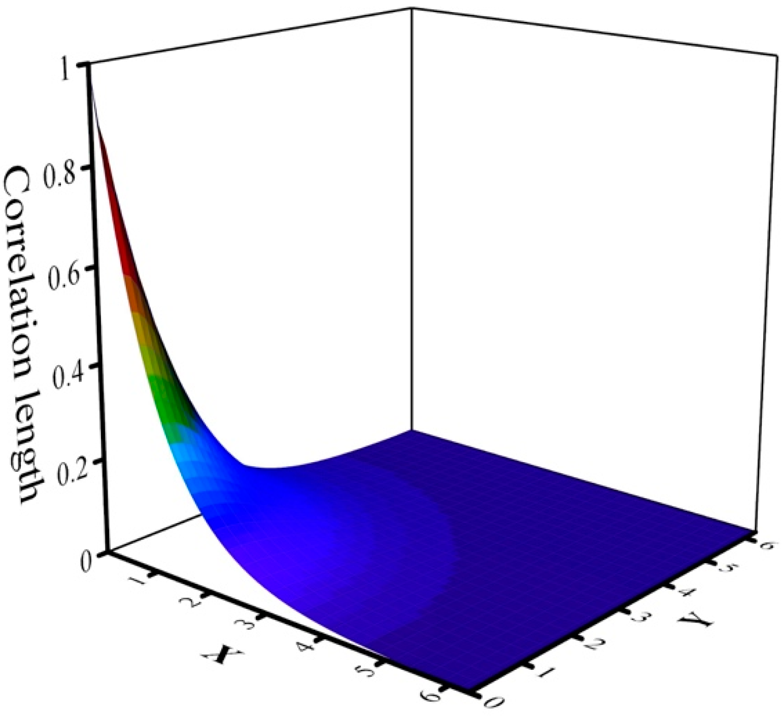
3.1. Spatial Correlation Model

The most common spatial correlation models of one-dimensional space are the exponential model, Gauss model, spherical model and second-order autoregressive model. The exponential model (also called Markovian decaying function) is used in this paper to describe the spatial correlation structure of the randomness of the soil. The formulas in one-dimensional and two-dimensional expressions are as follows:
ρ ( h ) = exp ( 2 d l )
ρ ( d x , d y ) = exp [ ( 2 d x l x ) 2 + ( 2 d y l y ) 2 ]
where ρ is the correlation coefficient of different positions, d is the separated distance in the random field, l is the correlation length, d x , d y are the separated distances along the horizontal direction and vertical direction, respectively, and l x , l y are the horizontal correlation length and vertical correlation length in two-dimensional space.
A plot of this exponential model in two-dimensional space is given in Figure 4, indicating the properties at two points separated by lx and ly.
Figure 4 shows that the soil properties will be almost the same if the distance between two points is very close. A large correlation length implies that the soil property is correlated over a large spatial extent, resulting in a smooth variation within the soil profile. On the other hand, a small correlation length indicates that the fluctuation of the soil property is serious.

3.2. Generation of Random Fields Using the Karhunen–Loeve Series Expansion Method

The spatial variability of random soils is represented by a random field model. Several common models have been developed and used to generate random fields such as the covariance matrix decomposition method [44,45,46], the local average subdivision method [9,47,48] and the Karhunen–Loeve (K-L) series expansion method [27,49,50,51]. This paper applies the following K-L series expansion method to generate the Gauss random field because of its efficiency and precision.
H ^ i ( x ) = μ X i + s X i H ^ i D ( x ) = μ X i + s X i j = 1 M λ j f j ( x ) χ j i
where H ^ i ( x ) is the desired random field considering the mean value μ X i and standard deviation s X i , i is the i-th random field, x is the spatial position, H ^ i D ( x ) is a standard Gaussian random field after discretizing the space, M is the number of series expansion terms of a random field, λ j and f j ( x ) are the j th eigenvalue and j th eigenfunction of spatial correlation model ρ , respectively, χ is a stochastic matrix of size M × N considering the autocorrelation of the random field, χ = ξ   L T , where ξ is a stochastic vector of size M × N in standard Gaussian space, and L is the lower triangular matrix obtained by the Cholesky decomposition of matrix ρ in standard Gaussian space, and its size is M × N .

3.3. Probability Distribution of Strength Parameters

The cohesion and internal friction angle are considered as random variables in this numerical model of slope stability for this test embankment.
Based on previous studies, the shear strength parameters, e.g., cohesion and internal friction angle in geotechnical engineering can be modeled as Gaussian distributions or log-normal distributions [5,31]. Since the shear strength parameters in geotechnical engineering are always positive, in this study, c and φ are assumed to be characterized statistically by a log-normal distribution defined by two mean values, μ c and μ φ , and two standard deviations s c and s φ , respectively. Once the mean and standard deviation are expressed in terms of the dimensionless COV, defined as COV = s / μ , the mean value and standard deviation of the underlying Gauss distribution of ln c and ln φ are given by [28,31,49],
s ln c = ln   ( 1 + COV c 2 )
μ ln c = ln   μ c 0.5 s c 2
and
s ln φ = ln   ( 1 + COV φ 2 )
μ ln φ = ln   μ φ 0.5 s φ 2

4. Results and Discussion

4.1. Monte Carlo Simulation

There are many stochastic methods for probabilistic slope analysis in previous studies, but the Monte Carlo simulation is still the most common technique. Even though a large amount of computing time is required to use this technology, the mathematical formulation of the Monte Carlo method is relatively simple.
During the process of probabilistic analysis, the finite element method with strength reduction technology is repeated enough times to reach a stable value. Figure 5 shows the convergence of the estimated mean value and standard deviation of FOS from 2000 Monte Carlo simulations for the test embankment slope. The result converges to a stable value when the number of Monte Carlo simulations reaches about 1000 from Figure 5. The 1000 random field will be generated during the 1000 Monte Carlo simulations; then, 1000 FOSs could be obtained based on the mean value, standard deviation and the spatial correlated structural of the strength parameters. The average of the 1000 FOSs will be used as the result to evaluate the stability. Indeed, there is still an error compared with the true solution; however, it is acceptable for geotechnical engineering. Therefore, all the results of FOS are obtained by performing Monte Carlo simulations 1000 times, for the balance of computing time and numerical error. These results are used to describe the probabilistic stability of the slope.

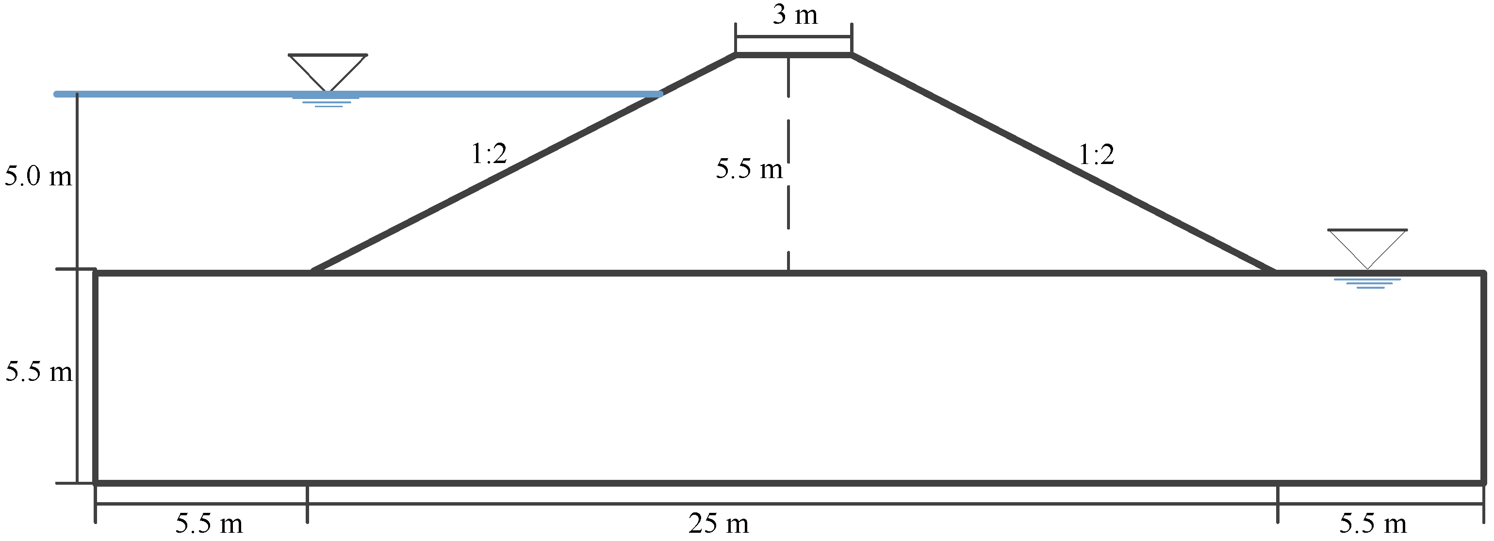
4.2. The Characters of a Test Embankment Slope

The instability of an embankment slope is a very complex physical process, which involves seepage, boundary conditions, pore water pressure, stress history of the soil and so on. Herein, the FOS of the embankment slope subjected to slow drawdown (implying that the excess pore water pressure is neglected) is studied considering the seepage and spatial variability of the soil.
The numerical modeling is conducted on a test embankment slope as shown in Figure 6. This embankment constructed on a 5.5 m thick soil foundation that is 5.5 m high, with upstream and downstream slopes of 2h:1v, and the water level (WL) in the river is 5 m above the foundation. To evaluate the stability of this embankment slope, the FOS is calculated by the finite element limit analysis with the strength reduction method mentioned in Section 2.4.
The soil properties are displayed in Table 1. The Young’s modulus E , Poisson ratio ν and hydraulic conductivity k s are assumed to be deterministic, as they have turned out to have little influence on the results of the slope stability analysis. Several previous studies [6,7] pointed out that ly is much smaller than lx in geotechnics, so that ly is fixed to 1 meter. The lx of the cohesion and internal friction angle is set at five different levels. In particular, the dilation angle is set to zero, corresponding to no volume change during the process of yielding.

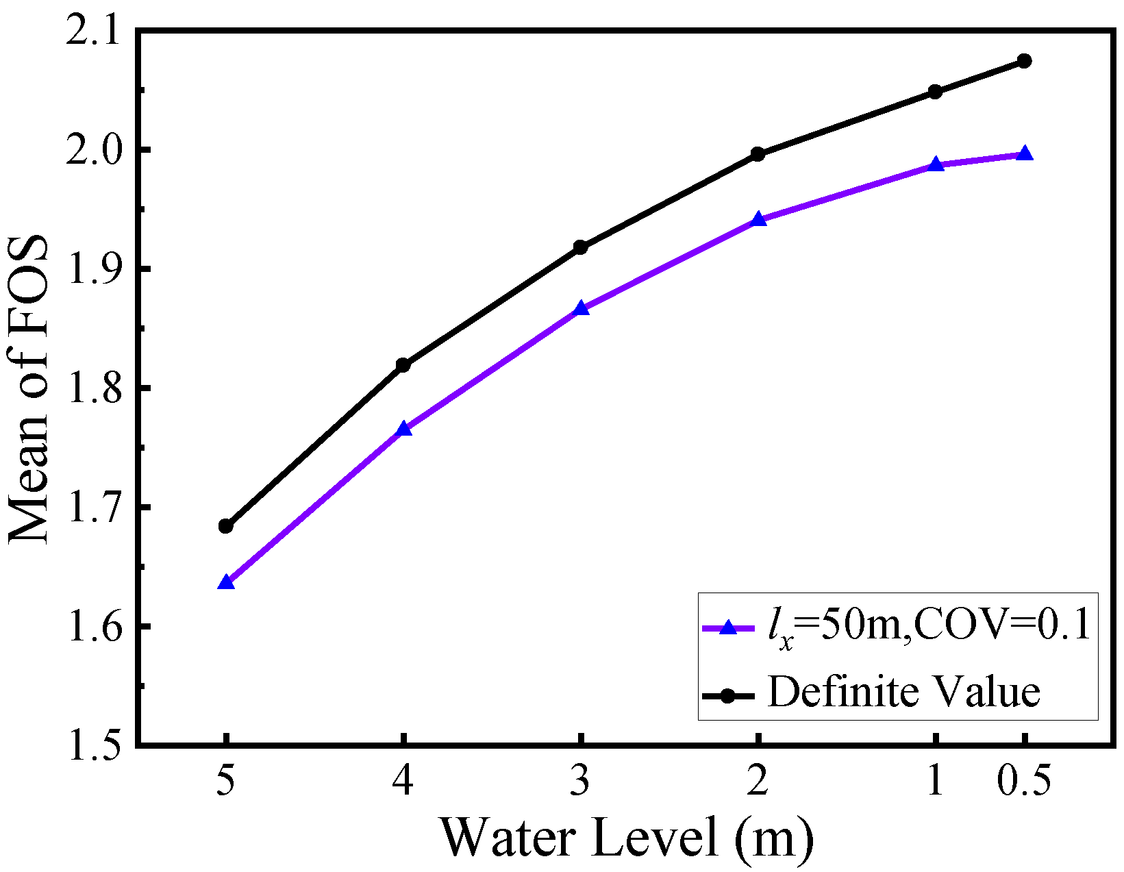
4.3. Deterministic Analysis Results

A series of deterministic analyses are carried out in OptumG2 before the probability analysis during the process of the slow drawdown of the WL. The finite element limit analysis with the mesh adaptivity technique is used for this numerical model. Figure 7 shows that the number of the adaptive finite elements in 2000 is suitable for obtaining stable FOSs.
Several different WLs are set to simulate the slow water drawdown, because the pore water pressure can completely dissipate during the process of water falling slowly. The FOSs of the embankment slope at six different WLs of 5 m, 4 m, 3 m, 2 m, 1 m, and 0.5 m are calculated to describe the slow water drawdown. As shown in Figure 8, the FOSs increase with the slow water drawdown. The reason is that it is assumed to be a steady-state seepage during the slow drawdown. The effective stress increases with the dissipation of pore water pressure, and the matric suction also increases during the slow drawdown. These two aspects will strengthen the stability of the embankment slope.
As mentioned in Section 2.4.3 of this paper, the upper and lower bound values of FOSs are calculated by strength reduction technology. The true solution then falls somewhere between the upper bound and lower bound values, and thus, the mean value of the upper and lower values is regarded as the true solution, as shown in Figure 8. The probabilistic results described in the following sections are also calculated using this method.

4.4. Analysis of Random Field Results

In this section, there are in total 150 random field analysis results obtained from five different lx and five different COVs under six different WLs. The detailed computational setup can be found in the Appendix A, and corresponding FOSs are displayed in Figure 9.
Furthermore, to compare with the deterministic results in Figure 8, during the slow water drawdown, one group of random field results with the parameter set, COV = 0.1, lx = 50 m, corresponding to six water levels are plotted as shown in Figure 10. It shows the variation of the statistical FOSs during the slow drawdown of the WL, during which the FOSs present a gradual upward trend with the decrease in the WL. Such a result comes from two reasons. The first one is that the effective stress of soil increases with the decrease in WL because the pore water pressure disappears. The other one is that the increase in mechanical bite force leads to the soil slope being more stable.
With the same WL, all FOSs obtained from the random field analysis are smaller than the results obtained from the deterministic analysis. In other words, the deterministic analysis method may sometimes overestimate the stability of the embankment slope, having potential risk. It implies that it is more reasonable to adopt the random field analysis, especially when the objective is the natural geomaterials. It is interesting to note that all the other results from the different parameter sets have a similar trend to Figure 10.

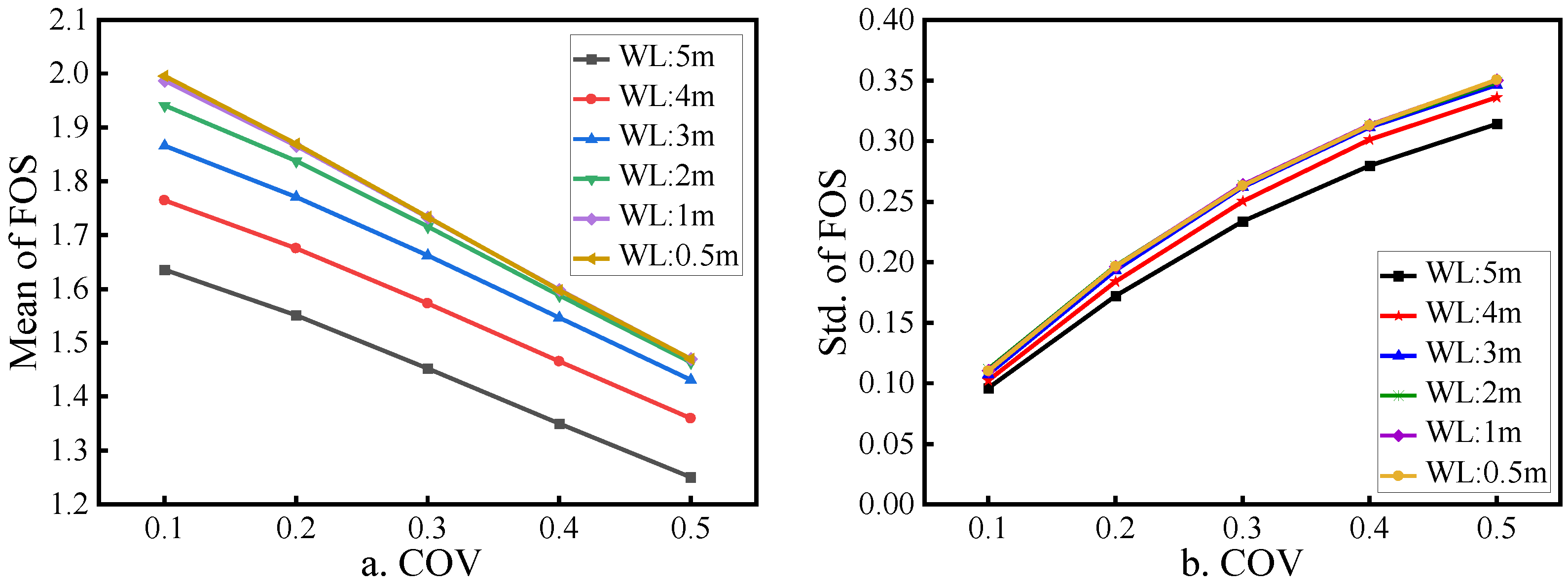
4.4.1. Effect of Different COV

Some literature studied that the shear strength parameters, cohesion and internal friction angle, in geotechnical materials varied from 0.1 to 0.5 [6]. The FOS is calculated, and the parametric study of the spatial variation of shear strength parameters is investigated during the slow water drawdown. All the results of the random field have similar properties with the histograms of the FOSs depicted in Figure 11, which correspond to the parameter set (lx = 50 m, WL = 5 m) versus five different COVs. For comparison, the same deterministic results were 1.684, as marked with an arrow in Figure 11. Figure 11 also shows that all the mean values in the five subfigures are lower than the deterministic value of 1.684. The differences between the mean value and deterministic value become larger with the increase in COV of shear strength. The statistical result from Figure 11 shows that although the FOS obtained from deterministic FOS is close to the mean value of that based on random field analysis, still nearly half of the FOSs are less than the deterministic value. The result from Figure 11e shows that there is a large difference between the mean value and the deterministic value, and the failure probability was about 23.3%. This result presents a high risk of landslides for the overall slope system, despite the mean value from the random field analysis and the deterministic value both being located at a relatively safe level. Figure 11 also shows that the range of FOSs increases with the increase in the COV, having similar properties to the previous study. The result also indicates that the random field method is a more reasonable method for assessing the stability of the geotechnical slope.
Figure 12 shows the contour of the shear dissipation energy at the last stage of the failure slope for this test embankment, in which the subfigures correspond to the subfigures in Figure 11. The shear strength of the soil set in this test embankment is strong because the FOS is relatively high, resulting in the failure of circular slip surface through the toe shown in Figure 12. The failure circular slip surface moved toward the bottom of the foundation with the COV of the shear strength becoming larger. In other words, the magnitude of the failure soil increased with the COV of the shear strength becoming larger.
Figure 13 shows that the mean FOS decreases as the COV increases. The reason is that when the COV becomes greater, the fluctuation of the uncertainty of the soil strength becomes more serious. It is more possible to take much weaker strength parameters, cohesion and internal friction angle, so that the FOS becomes lower. This is consistent with the real situation that there are strong and weak areas in an actual slope system. The failure of the embankment slope occurs easily in weak soil areas.

4.4.2. Effect of Different lx

Because of the long-term depositional process and load history, the spatial correlation structure of geomaterials should be considered as a basic property that cannot be ignored. In previous studies, the magnitude of the vertical correlation length ly which is from 1 to 2 m, is always lower than the horizontal correlation length lx, which is usually from 30 to 60 m [6]. In this paper, the ly is assumed to be 1 m as a fixed value, and the influence on the FOS of five different lx is mainly studied. Figure 14 shows five different random fields of cohesion generated by the K-L series expansion method. The obvious spatial correlation structure can be observed by the contours.
Figure 15 shows the variation of mean FOSs with lx for different COVs at the 5 m high water level. The mean FOSs slightly decrease with the increase in the lx for the range 1–50 m, and this is in good agreement with Zhu et al. [28]. The mean FOSs reach a minimum when the lx ranges from 30 to 50 m, because the width of the foundation of this test embankment in this paper is 36 m. The stability of this test model will almost not be influenced when the lx exceeds 50 m. Hence, the end part of the curve in Figure 11 tends to be horizontal. This is also consistent with real engineering, and the spatial correlation length is constant for a specific case, and the maximum length is no more than the outline. However, the standard deviation of FOS increases with the increase in lx. The increasing trend is obvious when the COV is high.

5. Conclusions

In this study, the finite element limit analysis was used to study the stability of embankment slopes subject to the slow water drawdown, considering the spatial variability of geomaterials. We assumed that the pore water pressure in the soil body has been dissipated during the slow drawdown. Hence, five different WLs were set to represent that the water level continues to drop.
The spatial variability of geomaterials is described by a random field model, which is determined by the mean, standard deviation and spatial correlation length of the shear strength cohesion and internal friction angle. Both the cohesion and internal friction angle are assumed to follow a log-normal distribution. The range of the COV is set from 0.1 to 0.5. The vertical correlation length is fixed at 1 m, and five different horizontal correlation lengths are set, namely 1 m, 30 m, 40 m, 50 m, and 500 m. All the mean values of FOS obtained from 1000 Monte Carlo simulations for different working conditions are lower than the corresponding deterministic analysis. The FOS increases with the decrease in the WL and decreases with the increase in COV. This is consistent with the actual situation that the shear failure surface is more likely to occur at the position where the soil strength is weaker. Although the mean value of FOS was greater than 1 for this test embankment, the probability of failure is still high, e.g., the probability of failure is 23.3% in Figure 11e.
The study shows that the probability of potential risk is high because the FOS obtained from the deterministic analysis is higher than the random field analysis result. Hence, it is more reasonable to evaluate the stability of an embankment slope using the probability framework rather than the deterministic analysis. Further work will focus on the influence of rapid water drawdown on slope stability as well as the random field action.

Author Contributions

Conceptualization, Q.Z.; Data curation, X.X.; Formal analysis, X.W.; Funding acquisition, Q.Z.; Methodology, X.X. and X.Z.; Software, X.Z.; Writing—original draft, X.W.; Writing—review & editing, X.G. All authors have read and agreed to the published version of the manuscript.

Funding

This research was funded by the National Natural Science Foundation of China (No. 12002118); the Fundamental Research Funds for the Central Universities (No. 2019B65814); the Research and Innovation Project for College Graduate of Jiangsu Province (No. SJKY19_0422); the National Key Research & Development Program of China (No. 2017YFC1502603).

Institutional Review Board Statement

This study does not require ethical approval.

Informed Consent Statement

Informed consent was obtained from all subjects involved in the study.

Data Availability Statement

The data presented in this study are available on request from the first author.

Acknowledgments

The author Xiaobing Wang also gratefully acknowledges the support from China Scholarship Council (No. 202006710049) and UK-Jiangsu 20+20 World Class University Consortium.

Conflicts of Interest

The authors declare no conflict of interest.

Abbreviations

b the body force vector
c the cohesion
c the cohesion after reduction
d the separated distance in random field
C O V coefficient of variation
E the elastic modulus
F the yield function
f s the factor of safety
f j ( x ) the jth eigenfunction
G the plastic potential function
H ^ ( x ) the desired random field
H ^ D ( x ) Gaussian random field
h the total head
h * the position head
k the hydraulic conductivity
l the correlation length
L the lower triangular matrix
M , N the number
p s the static water pressure
P the projection matrix
q x ,   q y the fluid velocity along the x and y directions
s standard deviation
S the boundary
t the tractions
t s the seepage pressure
u the displacement vector
u s the specified boundary displacement
V the configuration of interest
α the factor of load
γ d , γ sat the dry and saturate weight of soil
γ w the water gravity
ε the strain tensor
ε ˙ p the plasticity strain rate tensor
λ ˙ the plastic multiplier
λ j the jth eigenvalue
μ mean value
ξ the stochastic vector
ρ the correlation coefficient
ρ the matrix of correlation coefficient
σ the total stress tensor
σ the effective stresses
τ shear stress
ν the Poisson ratio
φ the internal friction angle
  φ   the internal friction angle after reduction
χ the stochastic matrix
ψ the dilation angle
κ the slack variables
the strain-displacement operator
T the equilibrium operator

Appendix A. The FOSs Obtained from Random Field Analysis

Table A1 shows all the random field analysis results. Each FOS in Table A1 is obtained from the mean value of 1000 Monte Carlo simulations upper bound limit analysis and 1000 Monte Carlo simulations lower bound limit analysis, respectively.
Table A1. The result of FOSs of random field.
COVWL/mHorizontal Correlation Length
1 m30 m40 m50 m500 m
0.151.6521.6351.6331.6361.636
41.7821.7651.7621.7651.765
31.8821.8651.8631.8661.866
21.9581.9401.9381.9411.941
12.0061.9841.9851.9871.996
0.52.0141.9911.9951.9962.012
0.251.5861.5491.5461.5511.551
41.7111.6741.6711.6761.676
31.8071.7701.7671.7711.772
21.8771.8351.8341.8381.843
11.9081.8601.8651.8661.890
0.51.9121.8641.8701.8701.903
0.351.5041.4501.4481.4521.451
41.6231.5701.5681.5731.572
31.7141.6591.6581.6621.663
21.7741.7061.7121.7161.729
11.7921.7241.7311.7331.768
0.51.7951.7251.7341.7341.778
0.451.4141.3481.3461.3501.350
41.5271.4641.4621.4661.466
31.6111.5451.5431.5471.551
21.6591.5821.5851.5881.610
11.6711.5881.5971.5991.644
0.51.6721.5871.5981.5981.651
0.551.3211.2481.2471.2501.252
41.4271.3591.3581.3601.364
31.5041.4271.4281.4311.442
21.5411.4541.4601.4641.495
11.5471.4571.4681.4701.523
0.51.5481.4541.4681.4701.528

References

  1. Bishop, A.W. The use of the slip circle in the stability analysis of slopes. Geotechnique 1955, 5, 7–17. [Google Scholar] [CrossRef]
  2. Duncan, J.M.; Wright, S.G. The accuracy of equilibrium methods of slope stability analysis. Eng. Geol. 1980, 16, 5–17. [Google Scholar] [CrossRef]
  3. Mahmood, K.; Kim, J.M.; Ashraf, M. The effect of soil type on matric suction and stability of unsaturated slope under uniform rainfall. KSCE J. Civ. Eng. 2016, 20, 1294–1299. [Google Scholar] [CrossRef]
  4. Ijaz, N.; Ye, W.; Rehman, Z.U.; Dai, F.; Ijaz, Z. Numerical study on stability of lignosulphonate-based stabilized surficial layer of unsaturated expansive soil slope considering hydro-mechanical effect. Transp. Geotech. 2022, 32, 100697. [Google Scholar] [CrossRef]
  5. Elkateb, T.; Chalaturnyk, R.; Robertson, P.K. An overview of soil heterogeneity: Quantification and implications on geotechnical field problems. Can. Geotech. J. 2003, 40, 1–15. [Google Scholar] [CrossRef]
  6. Phoon, K.K.; Kulhawy, F.H. Characterization of geotechnical variability. Can. Geotech. J. 1999, 36, 612–624. [Google Scholar] [CrossRef]
  7. Baecher, G.B.; Christian, J.T. Reliability and Statistics in Geotechnical Engineering; John Wiley & Sons Ltd: ChiChester, UK, 2003. [Google Scholar]
  8. Srivastava, A.; Babu, G.L.S.; Haldar, S. Influence of spatial variability of permeability property on steady state seepage flow and slope stability analysis. Eng. Geol. 2010, 110, 93–101. [Google Scholar] [CrossRef]
  9. Li, J.H.; Zhou, Y.; Zhang, L.L.; Tian, Y.; Cassidy, M. Random finite element method for spudcan foundations in spatially variable soils. Eng. Geol. 2016, 205, 146–155. [Google Scholar] [CrossRef]
  10. Cassidy, M.J.; Uzielli, M.; Tian, Y. Probabilistic combined loading failure envelopes of a strip footing on spatial variable soil. Comput. Geotech. 2013, 49, 191–205. [Google Scholar] [CrossRef]
  11. Li, D.Q.; Yang, Z.Y.; Cao, Z.J.; Au, S.-K.; Phoon, K.-K. System reliability analysis of slope stability using generalized Subset Simulation. Appl. Math. Model. 2017, 46, 650–664. [Google Scholar] [CrossRef]
  12. Tang, C.; Phoon, K.K.; Zhang, L.; Li, D.-Q. Model uncertainty predicting the bearing capacity of sand overlying clay. Int. J. Geomech. 2017, 17, 04017015. [Google Scholar] [CrossRef]
  13. Xiao, T.; Li, D.Q.; Cao, Z.J.; Tang, X.-S. Full probabilistic design of slopes in spatially variable soils using simplified reliability analysis method. Georisk 2017, 11, 146–159. [Google Scholar] [CrossRef]
  14. Nefeslioglu, H.A.; Gokceoglu, C. Probabilistic risk assessment in medium scale for rainfall-induced earthflows: Catakli Catchment Area (Cayeli, Rize, Turkey). Math. Probl. Eng. 2011, 2011. [Google Scholar] [CrossRef] [Green Version]
  15. Rosenblueth, E. Point estimates for probability moments. Proc. Natl. Acad. Sci. USA 1975, 72, 3812–3814. [Google Scholar] [CrossRef] [PubMed] [Green Version]
  16. Connor Langford, J.; Diederichs, M.S. Reliability based approach to tunnel lining design using a modified point estimated method. Int. J. Rock Mech. Min. Sci. 2013, 60, 263–276. [Google Scholar] [CrossRef]
  17. Chen, Z.; Du, J.; Yan, J.; Sun, P.; Li, K.; Li, Y. Point estimation method: Validation, efficiency improvement, and application to embankment slope stability reliability analysis. Eng. Geol. 2019, 263, 105232. [Google Scholar] [CrossRef]
  18. Lanzafame, R.; Sitar, N. Reliability analysis of the influence of seepage on levee stability. Environ. Geotech. 2019, 6, 284–293. [Google Scholar] [CrossRef]
  19. Jia, J.; Wang, S.; Zheng, C.; Chen, Z.; Wang, Y. FOSM-based shear reliability analysis of GSGR dams using strength theory. Comput. Geotech. 2018, 97, 52–61. [Google Scholar] [CrossRef]
  20. Cho, S.E. Effects of spatial variability of soil properties on slope stability. Eng. Geol. 2007, 92, 97–109. [Google Scholar] [CrossRef]
  21. Ahmed, A.; Soubra, A.H. Probabilistic analysis at the serviceability limit state of two neighboring strip footings resting on a spatially random soil. Struct. Saf. 2014, 49, 2–9. [Google Scholar] [CrossRef]
  22. Fenton, G.A.; Griffiths, D.V. Statistics of block conductivity through a simple bounded stochastic medium. Water Resour. Res. 1993, 29, 1825–1830. [Google Scholar] [CrossRef] [Green Version]
  23. Griffiths, D.V.; Fenton, G.A. Probabilistic slope stability analysis by finite element. J. Geotech. Geoenviron. Eng. 2004, 130, 507–518. [Google Scholar] [CrossRef] [Green Version]
  24. Griffiths, D.V.; Huang, J.; Fenton, G.A. Influence of spatial variability on slope reliability using 2-D random fields. J. Geotech. Geoenviron. Eng. 2009, 135, 1367–1378. [Google Scholar] [CrossRef] [Green Version]
  25. Huang, J.; Griffiths, D.V.; Fenton, G.A. System reliability of slope by RFEM. Soils Found. 2010, 50, 343–353. [Google Scholar] [CrossRef] [Green Version]
  26. Griffiths, D.V.; Huang, J.; Fenton, G.A. Probabilistic infinite slope analysis. Comput. Geotech. 2011, 38, 577–584. [Google Scholar] [CrossRef]
  27. Cho, S.E. Probabilistic analysis of seepage that considers the spatial variability of permeability for an embankment on soil foundation. Eng. Geol. 2012, 133–134, 30–39. [Google Scholar] [CrossRef]
  28. Zhu, H.; Zhang, L.M.; Zhang, L.L.; Zhou, C.B. Two-dimensional probabilistic infiltration analysis with a spatial varying permeability function. Comput. Geotech. 2013, 48, 249–259. [Google Scholar] [CrossRef]
  29. Tan, X.; Wang, X.; Khoshnevisan, S.; Hou, X.; Zha, F. Seepage analysis of earth dams considering spatial variability of hydraulic parameters. Eng. Geol. 2017, 228, 260–269. [Google Scholar] [CrossRef]
  30. Mouyeaux, A.; Carvajal, C.; Bressolette, P.; Peyras, L.; Breul, P.; Bacconnet, C. Probabilistic analysis of pore water pressures of an earth dam using a random finite element approach based on field data. Eng. Geol. 2019, 259, 105190. [Google Scholar] [CrossRef]
  31. Wang, M.Y.; Liu, Y.; Ding, Y.N.; Yi, B.-L. Probabilistic stability analyses of multi-stage soil slopes by bivariate random fields and finite element methods. Comput. Geotech. 2020, 122, 103529. [Google Scholar] [CrossRef]
  32. Li, D.; Li, L.; Cheng, Y.; Hu, J.; Lu, S.; Li, C.; Meng, K. Reservoir slope reliability analysis under water level drawdown considering spatial variability and degradation of soil properties. Comput. Geotech. 2022, 151, 104947. [Google Scholar] [CrossRef]
  33. Sloan, S.W. Lower bound limit analysis using finite elements and linear programming. Int. J. Numer. Anal. Methods Geomech. 1988, 12, 61–77. [Google Scholar] [CrossRef]
  34. Sloan, S.W. Upper bound limit analysis using finite elements and linear programming. Int. J. Numer. Anal. Methods Geomech. 1989, 13, 263–282. [Google Scholar] [CrossRef]
  35. Huang, J.; Lyamin, A.V.; Griffiths, D.V.; Krabbenhoft, K.; Sloan, S. Quantitative risk assessment of landslide by limit analysis and random fields. Comput. Geotech. 2013, 53, 60–67. [Google Scholar] [CrossRef]
  36. Krabbenhoft, K.; Lyamin, A.V. Strength reduction finite-element limit analysis. Géotech. Lett. 2015, 5, 250–253. [Google Scholar] [CrossRef]
  37. Chen, Z.H.; Lei, J.; Huang, J.H.; Cheng, X.H.; Zhang, Z.C. Finite element limit analysis of slope stability considering spatial variability of soil strengths. Chin. J. Geotech. Eng. 2018, 40, 985–993. [Google Scholar]
  38. Qian, Z.G.; Li, A.J.; Chen, W.C.; Lyamin, A.; Jiang, J. An artificial neural network approach to inhomogeneous soil slope stability predictions based on limit analysis methods. Soils Found. 2019, 59, 556–569. [Google Scholar] [CrossRef]
  39. Krabbenhoft, K.; Lyamin, A.; Krabbenhoft, J. OptumG2: Theory, Optum Computational Engineering, Version 2016; Optum Computational Engineering: Copenhagen, Denmark, 2018. [Google Scholar]
  40. Makrodimopoulos, A.; Martin, C. Limit analysis using large-scale SOCP optimization. In Proceedings of the 13th ACME conference: University of Sheffield, Sheffield, UK, 21–22 March 2005. [Google Scholar]
  41. Zhang, X.; Krabbenhoft, K.; Pedroso, D.M.; Lyamin, A.; Sheng, D.; da Silva, M.V.; Wang, D. Particle finite element analysis of large deformation and granular flow. Comput. Geotech. 2013, 53, 133–142. [Google Scholar] [CrossRef]
  42. Krabbenhoft, K. OptumG2; OptumCE Optum Computational Engineering: Copenhagen, Denmark, 2020; Available online: www.optumce.com (accessed on 1 September 2020).
  43. Liu, S.Y.; Shao, L.T.; Li, H.J. Slope stability analysis using the limit equilibrium method and two finite element methods. Comput. Geotech. 2015, 63, 291–298. [Google Scholar] [CrossRef]
  44. Green, D.K.E.; Douglas, K.; Mostyn, G. The simulation of discretization of random fields for probabilistic finite element analysis of soils using meshes of arbitrary triangular elements. Comput. Geotech. 2015, 68, 91–108. [Google Scholar] [CrossRef]
  45. Jiang, S.H.; Huang, J.S. Efficient slope reliability analysis at low-probability levels in spatially variable soils. Comput. Geotech. 2016, 75, 18–27. [Google Scholar] [CrossRef]
  46. Halder, K.; Chakraborty, D. Probabilistic bearing capacity of strip footing on reinforced anisotropic soil slope. Geomech. Eng. 2020, 23, 15–30. [Google Scholar] [CrossRef]
  47. Fenton, G.A.; Vanmarcke, E.H. Simulation of random fields via local average subdivision. J. Eng. Mech. 1990, 116, 1733–1749. [Google Scholar] [CrossRef] [Green Version]
  48. Frimpong, S.; Achireko, P.K. Conditional LAS stochastic simulation of regionalized variables in random fields. Comput. Geosci. 1998, 2, 37–45. [Google Scholar] [CrossRef]
  49. Shi, L.S.; Yang, J.Z.; Chen, F.L.; Zhou, F.C. Research on application of Karhunen-Loeve expansion to simulating anisotropic random field of soil property. Rock Soil Mech. 2007, 28, 2303–2308. [Google Scholar]
  50. Johari, A.; Sabzi, A. Reliability analysis of foundation settlement by stochastic response surface and random finite-element method. Sci. Iran. Trans. A Civ. Eng. 2017, 24, 2741–2751. [Google Scholar] [CrossRef]
  51. Tan, X.H.; Dong, X.L.; Fei, S.Z.; Gong, W.P.; Xiu, L.T.; Hou, X.L.; Ma, H.C. Reliability analysis method based on KL expansion and its application. Chin. J. Geotech. Eng. 2020, 42, 808–816. [Google Scholar]
Figure 1. The lower bound element.
Applsci 12 10282 g001
Figure 2. The upper bound element.
Applsci 12 10282 g002
Figure 3. The process of strength reduction for Mohr–Coulomb constitutive.
Applsci 12 10282 g003
Figure 4. The spatial correlation model in two-dimensional space (X: dx/lx; Y: dy/ly).
Applsci 12 10282 g004
Figure 5. Convergence of FOS using Monte Carlo simulation ((a) The Mean of FOS for 2000 Monte Carlo simulations; (b) The Std. of FOS for 2000 Monte Carlo simulations).
Applsci 12 10282 g005
Figure 6. Plane computational model of a test embankment.
Applsci 12 10282 g006
Figure 7. The choice of element number.
Applsci 12 10282 g007
Figure 8. The results of deterministic analysis.
Applsci 12 10282 g008
Figure 9. The result of FOSs from random field analysis.
Applsci 12 10282 g009
Figure 10. The FOS vs. different WLs for definite and random field analysis.
Applsci 12 10282 g010
Figure 11. Histogram of the FOSs obtained from 1000 realizations for the set (WL = 5 m, lx = 50 m): (a) COV = 0.1; (b) COV = 0.2; (c) COV = 0.3; (d) COV = 0.4; (e) COV = 0.5.
Applsci 12 10282 g011
Figure 12. The contours of shear dissipation energy based on lx = 50 m, WL = 5 m: (a) COV = 0.1; (b) COV = 0.2; (c) COV = 0.3; (d) COV = 0.4; (e) COV = 0.5.
Applsci 12 10282 g012
Figure 13. FOSs vs. COV of shear strength for different WLs (lx = 50 m) ((a) The Mean of FOS for six different WLs; (b) The Std. of FOS for six different WLs).
Applsci 12 10282 g013
Figure 14. Typical realizations of the random field of cohesion ( μ c = 15 kPa ,       σ c = 5 kPa ) for different lx ((a) lx = 1 m, (b) lx = 30 m, (c) lx = 40 m, (d) lx = 50 m, (e) lx = 500 m).
Applsci 12 10282 g014
Figure 15. FOS vs. lx for different COVs (WL = 5 m) ((a) The Mean of FOS for five different COVs; (b) The Std. of FOS for five different COVs).
Applsci 12 10282 g015
Table 1. Statistical properties of soil parameters.
ParameterMeanCoefficient of VariationHorizontal Correlation Length
c (kPa)150.1, 0.2, 0.3, 0.4, 0.51 m, 30 m, 40 m, 50 m, 500 m
φ   ( ° ) 200.1, 0.2, 0.3, 0.4, 0.51 m, 30 m, 40 m, 50 m, 500 m
E (MPa)40--
ν 0.3--
γ d   ( kN / m 3 )18--
γ sat   ( kN / m 3 )20--
ks (m/s)2 × 10−6--
Publisher’s Note: MDPI stays neutral with regard to jurisdictional claims in published maps and institutional affiliations.

