Article

Crouch Gait Analysis and Visualization Based on Gait Forward and Inverse Kinematics

by
Juan-Carlos Gonzalez-Islas
1,2,
Omar-Arturo Dominguez-Ramirez
1,*,
Omar Lopez-Ortega
1,
Jonatan Peña-Ramirez
3,
Jesus-Patricio Ordaz-Oliver
1 and
Francisco Marroquin-Gutierrez
4
1
Basic Sciences and Engineering Institute, Autonomous University of the State of Hidalgo, Hidalgo 42184, Mexico
2
Electromechanical Area, Technological University of Tulancingo, Hidalgo 43642, Mexico
3
Department of Systems and Control Engineering, School of Engineering, Tokyo Institute of Technology, Tokyo 152-8552, Japan
4
Consejo Nacional de Ciencia y Tecnologia CONACYT, Mexico City 03940, Mexico
*
Author to whom correspondence should be addressed.
Appl. Sci. 2022, 12(20), 10197; https://doi.org/10.3390/app122010197
Submission received: 13 September 2022 / Revised: 1 October 2022 / Accepted: 7 October 2022 / Published: 11 October 2022
(This article belongs to the Special Issue Biomechanics and Human Motion Analysis)

Abstract

:
Crouch gait is one of the most common gait abnormalities; it is usually caused by cerebral palsy. There are few works related to the modeling of crouch gait kinematics, crouch gait analysis, and visualization in both the workspace and joint space. In this work, we present a quaternion-based method to solve the forward kinematics of the position of the lower limbs during walking. For this purpose, we propose a modified eight-DoF human skeletal model. Using this model, we present a geometric method to calculate the gait inverse kinematics. Both methods are applied for gait analysis over normal, mild, and severe crouch gaits, respectively. A metric-based comparison of workspace and joint space for the three gaits for a gait cycle is conducted. In addition, gait visualization is performed using Autodesk Maya for the three anatomical planes. The obtained results allow us to determine the capabilities of the proposed methods to assess the performance of crouch gaits, using a normal pattern as a reference. Both forward and inverse kinematic methods could ultimately be applied in rehabilitation settings for the diagnosis and treatment of diseases derived from crouch gaits or other types of gait abnormalities.

1. Introduction

Human gait analysis (GA) is the systematic study of human walking [1]. Recently, instrumentation and computing technologies used to measure, process, and analyze body kinetics and kinematics have improved the efficiency of this assessment tool [2]. In clinical settings, gait analysis through kinetics and kinematics has been used to assess the effects of hip arthroplasty [3], stroke [4,5], osteoarthritis [6], Achilles tendinopathy [7], rheumatoid arthritis (RA) [8], inversion sprains [9], and Parkinson’s disease [10,11], among others. Human motion estimation sensing is a challenging issue for gait analysis. For example, in [12], an inertial wearable is used to estimate model-based inverse kinematics. In the same sense, other studies have used Magnetic Resonance Imaging (MRI) [13] and motion capture marker-based systems [14,15] to collect gait data in patients with cerebral palsy [13].
Crouch gait (CG) is one of the most common gait abnormalities, and is observed in people with cerebral palsy [16]; it is mainly characterized by excessive flexion of the hip, knee, and ankle [17,18,19]. In addition, crouch gait is distinguished in persons with hemiplegia after ischemic stroke [20]. CG causes joint pain [21] and arthritis [22], and is less efficient than a normal gait pattern [23]. Most of the works in the literature define a crouch gait only based on the knee position. Furthermore, kinematic parameters are well-defined when objective values of knee flexion are provided. However, few papers have considered these data and both lower limbs during the analysis [24], and consider the pathological gait patterns only in the sagittal plane. Other anatomical planes which could allow a crouch gait to be determined [18], such as the frontal and transverse planes, have not been considered.
Gait kinematics is the study of the mechanical movements of the musculoskeletal system during walking without considering the forces and moments that originate it [1]. The two types of kinematic problems are classed as forward and inverse kinematics. Forward kinematics is the calculation of the end point of a linked structure from the known position of the joint parameters and segment lengths.
On the other hand, inverse kinematics (IK) is the calculation of the joint parameters from the known position of the endpoint and segment lengths [25]. In robotics, inverse kinematics is used to determine the robot’s capability, efficiency, and accuracy. For this purpose, analytical and numerical approaches have been developed to solve this complex problem. Analytical methods include closed-form and algebraic elimination-based algorithms [26], while numerical algorithms such as Newton–Raphson [27], Jacobian transpose [28], and damped least squares [29] converge to a single solution for IK. In [14], an inverse kinematics method for lower limb kinematics over the sagittal plane using Groebner Basis theory is proposed. For robotic manipulators, these methods fail with complex joint geometries or can produce run-time errors. In addition, quaternions have been used to perform orientations and rotations of objects in 3D space [30] in areas such as computer graphics, multirotor tracking, control approaches, and the kinematics and dynamics of rigid bodies [31]. The most widely used methods in robot kinematics are homogeneous transformation and Denavit–Hartenberg (DH). However, the free representation and gimbal lock avoidance of quaternions have led to their use being optimal for this purpose [32].
The conventional gait model (CGM) [33] is very useful in clinical gait laboratories. In direct kinematics (DK) methods, CGM is used to calculate joint kinematics. Meanwhile, for inverse kinematics (IK), musculoskeletal modeling approaches to obtain joint angles are used. It is recommended that the same anatomical model be used for kinematic and musculoskeletal analysis to ensure consistency between both spaces [13]. Therefore, many studies have analyzed the kinematics and kinetics of ankles and knees, specifically in the sagittal plane [14,15,34,35,36,37,38,39]. This allows for a local analysis, however, for better assessment of abnormal gaits such as crouch gait, the other planes are necessary.
These issues make it necessary for crouch gait analysis to define kinematic gait patterns over the three anatomical planes in both the joint space and in the workspace. In addition, gait kinematics research focuses on building body models to explain the functioning of the body system and provide solutions to improve the methods for GA. Acquiring and analyzing kinematic and kinetic data of the body segments and joints of interest is a common procedure [40]. Tired and repetitive routines as well as lack of feedback on performance and improvement during rehabilitation very often lead the patient to discontinue the therapy [41]. In these cases, visualization [42] and exergaming (exercise + game) [43,44,45] platforms may improve the results of the rehabilitation process.
In this work, we propose a quaternions-based method to solve the forward kinematics of the position of the lower limbs during walking. We use an eight Degrees of Freedom (DoF) reduced gait model. In addition, we present an approach to solving the inverse kinematics for the same eight-DoF model and the visualization on the three anatomical planes of performance in both the workspace and the joint space. In this paper, forward and inverse kinematics analysis based on workspace and joint space metrics and visualization is carried out over the crouch gait. However, these methods could be extended for other abnormal gaits. This paper is organized as follows. Section 2 introduces the mathematics of forward and inverse kinematics modeling. Section 3 presents the main results. Section 4 provides a discussion, highlighting potential clinical applications. Finally, conclusions and possible future works are presented in Section 5.

2. Materials and Methods

An overview of the work presented in this paper is shown in Figure 1. First, the quaternion-based method used to calculate the forward kinematics of position is developed. To validate this method, the joint angles of the normal, mild crouch, and severe crouch gaits of the well-known 2392- O p e n S i m model are taken as input. Then, a visualization and analysis using fourth-dimensional (4D) plots (x, y, z and % gait cycle) and metrics in Cartesian space is developed. After that, the inverse kinematics algorithm is presented; to assess the approach, in this work we consider the Cartesian coordinates from the previous step as the inputs during this stage. However, Cartesian coordinates can be obtained from a motion marker-based system as well, which includes the image acquisition stage and processing units (see Figure 1). The performance in this space is assessed using joint angle metrics and 3D gait visualization in the three anatomical planes. A detailed description of the framework is presented next.

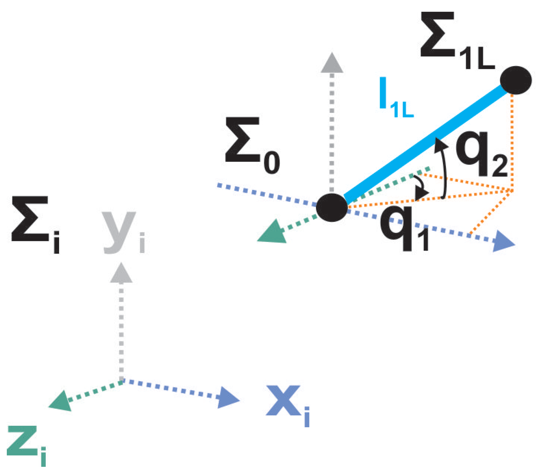
2.1. Gait Forward Kinematics

The gait kinematics analysis proposed in this work uses a robotics approach considering an eight-DoF simplified version of the conventional gait model [33] presented in Figure 2. First, the correspondences between the anatomical reference planes and three fundamental directions [2] with the 3D Cartesian space of the model (see Figure 2) are (anterior, x + ; superior, y + ; right, z + ) and (sagittal, X Y ; frontal, Y Z ; transverse, X Z ), respectively. The eight-DoF model features both the left and right lower limbs as eight rigid-body segments: the right pelvis ( l 1 R ), right femur ( l 2 R ), right tibia ( l 3 R ), right foot ( l 4 R ), left pelvis ( l 1 L ), left femur ( l 2 L ), left tibia ( l 3 L ), and left foot ( l 4 L ). In this work, the eight movements and their corresponding angles and rotation axis are: pelvic rotation ( q 1 , y 0 ), lateral pelvic list ( q 2 , x 0 ), right hip flexoextension ( q 3 R , z 1 R ), right knee flexoextension ( q 4 R , z 2 R ), right ankle dorsi/plantar flexion ( q 5 R , z 3 R ), left hip flexoextension ( q 3 L , z 1 L ), left knee flexoextension ( q 4 L , z 2 L ), and left ankle dorsi/plantar flexion ( q 5 L , z 3 L ). This approach could be extended to model the pelvic tilt movement as well as other joint movements. In this paper, we do not consider the surface constraints on gait kinematics.

2.1.1. Quaternions Algebra for Rotations

A quaternion can be expressed into the H four-dimensional space as H : = R + R i + R j + R k , where i = ( 1 , 0 , 0 ) , j = ( 0 , 1 , 0 ) and k = ( 0 , 0 , 1 ) are called the principal imaginaries and obey Hamilton’s rules, i.e., i 2 = j 2 = k 2 = i j k = 1 . Multiplication of these imaginaries resembles a cross-product i j = k , j k = i , k i = j , j i = k , k j = i , i k = j . A quaternion Q = r + x i + y j + z k consists of a real part a = r and a purely imaginary part v = x i + y j + z k . Quaternions with a zero real part are called pure quaternions. They can be written as Q = a + v and decomposed into Q = a + b u , which resembles a complex number, where u = [ x , y , z ] T / b = x v i + y v j + z v k is a unit three-vector and u = 1 . Q ¯ = Q 1 = a b u is known as the conjugate quaternion [30].
A rotation of an angle q about an axis u can be represented as the following unit quaternion:
Q = cos q 2 + u sin q 2 ,
for which the unit conjugate quaternion is
Q ¯ = cos q 2 u sin q 2 ,
Thus, the rotation to an arbitrary vector (pure quaternion) v R 3 is provided by the quaternion multiplication
R ( Q ) v = Q v Q ¯ .

2.1.2. Gait Forward Kinematics Using Quaternions Algebra

Gait forward kinematics of position allow the calculation of the position of the reference joints of the lower limbs in the workspace. To this end, the use of quaternions makes it possible to recursively calculate the Cartesian coordinates of these positions without the problems associated with the use of conventional methods when the number of degrees of freedom increases.
A quaternionic representation can be used for solving the forward kinematics of the position of the joint references. The home position of the frames of each reference can be represented as follows: pelvic Σ 0 = 0 + 0 i + 0 j + 0 k (global frame), right hip Σ 1 R = 0 + 0 i + 0 j + L 1 R k , right knee Σ 2 R = 0 + 0 i L 2 R j + 0 k , right ankle Σ 3 R = 0 + 0 i L 3 R j + 0 k , right toe Σ 4 R = 0 + L 4 R i 0 j + 0 k , left hip Σ 1 L = 0 + 0 i + 0 j L 1 L k , left knee Σ 2 L = 0 + 0 i L 2 L j + 0 k , left ankle Σ 3 L = 0 + 0 i L 3 L j + 0 k , and left toe Σ 4 L = 0 + L 4 L i 0 j + 0 k . We assume that the offset of the position of the pelvis frame in the ( y a x i s ) due to anthropometric values and gait abnormalities as a given, that is, Σ 0 is the global frame to model any gait using the eight-DoF kinematic chain. Now, it is possible to define each quaternion of rotation Q i regarding its respective angle q i , provided by
Q 1 = cos q 1 2 + sin q 1 2 j ,
Q 2 = cos q 2 2 + sin q 2 2 i ,
Q 3 R = cos q 3 R 2 + sin q 3 R 2 k ,
Q 4 R = cos q 4 R 2 + sin q 4 R 2 k ,
Q 5 R = cos q 5 R 2 + sin q 5 R 2 k ,
Q 3 L = cos q 3 L 2 + sin q 3 L 2 k ,
Q 4 L = cos q 4 L 2 + sin q 4 L 2 k ,
Q 5 L = cos q 5 L 2 + sin q 5 L 2 k .
Therefore, recursively, by using (3) the serial Cartesian coordinates of each joint reference after rotations for both lower limbs can be obtained using the following equations:
R ( Q ) Σ 1 R = Q 1 Q 2 Σ 1 R Q 2 ¯ Q 1 ¯ ,
R ( Q ) Σ 2 R = Q 1 Q 2 Σ 1 R Q 2 ¯ Q 1 ¯ + Q 1 Q 2 Q 3 R Σ 2 R Q 3 R ¯ Q 2 ¯ Q 1 ¯ ,
R ( Q ) Σ 3 R = Q 1 Q 2 Σ 1 R Q 2 ¯ Q 1 ¯ + Q 1 Q 2 Q 3 R Σ 2 R Q 3 R ¯ Q 2 ¯ Q 1 ¯ + Q 1 Q 2 Q 3 R Q 4 R Σ 3 R Q 4 R ¯ Q 3 R ¯ Q 2 ¯ Q 1 ¯ ,
R ( Q ) Σ 4 R = Q 1 Q 2 Σ 1 R Q 2 ¯ Q 1 ¯ + Q 1 Q 2 Q 3 R Σ 2 R Q 3 R ¯ Q 2 ¯ Q 1 ¯ + Q 1 Q 2 Q 3 R Q 4 R Σ 3 R Q 4 R ¯ Q 3 R ¯ Q 2 ¯ Q 1 ¯ + Q 1 Q 2 Q 3 R Q 4 R Q 5 R Σ 4 R Q 5 R ¯ Q 4 R ¯ Q 3 R ¯ Q 2 ¯ Q 1 ¯ ,
R ( Q ) Σ 1 L = Q 1 Q 2 Σ 1 L Q 2 ¯ Q 1 ¯ ,
R ( Q ) Σ 2 L = Q 1 Q 2 Σ 1 L Q 2 ¯ Q 1 ¯ + Q 1 Q 2 Q 3 L Σ 2 L Q 3 L ¯ Q 2 ¯ Q 1 ¯ ,
R ( Q ) Σ 3 L = Q 1 Q 2 Σ 1 L Q 2 ¯ Q 1 ¯ + Q 1 Q 2 Q 3 L Σ 2 L Q 3 L ¯ Q 2 ¯ Q 1 ¯ + Q 1 Q 2 Q 3 L Q 4 L Σ 3 L Q 4 L ¯ Q 3 L ¯ Q 2 ¯ Q 1 L ¯ ,
R ( Q ) Σ 4 L = Q 1 Q 2 Σ 1 L Q 2 ¯ Q 1 ¯ + Q 1 Q 2 Q 3 L Σ 2 L Q 3 L ¯ Q 2 ¯ Q 1 ¯ + Q 1 Q 2 Q 3 R Q 4 L Σ 3 L Q 4 L ¯ Q 3 L ¯ Q 2 ¯ Q 1 ¯ + Q 1 Q 2 Q 3 L Q 4 L Q 5 L Σ 4 L Q 5 L ¯ Q 4 L ¯ Q 3 L ¯ Q 2 ¯ Q 1 ¯ .

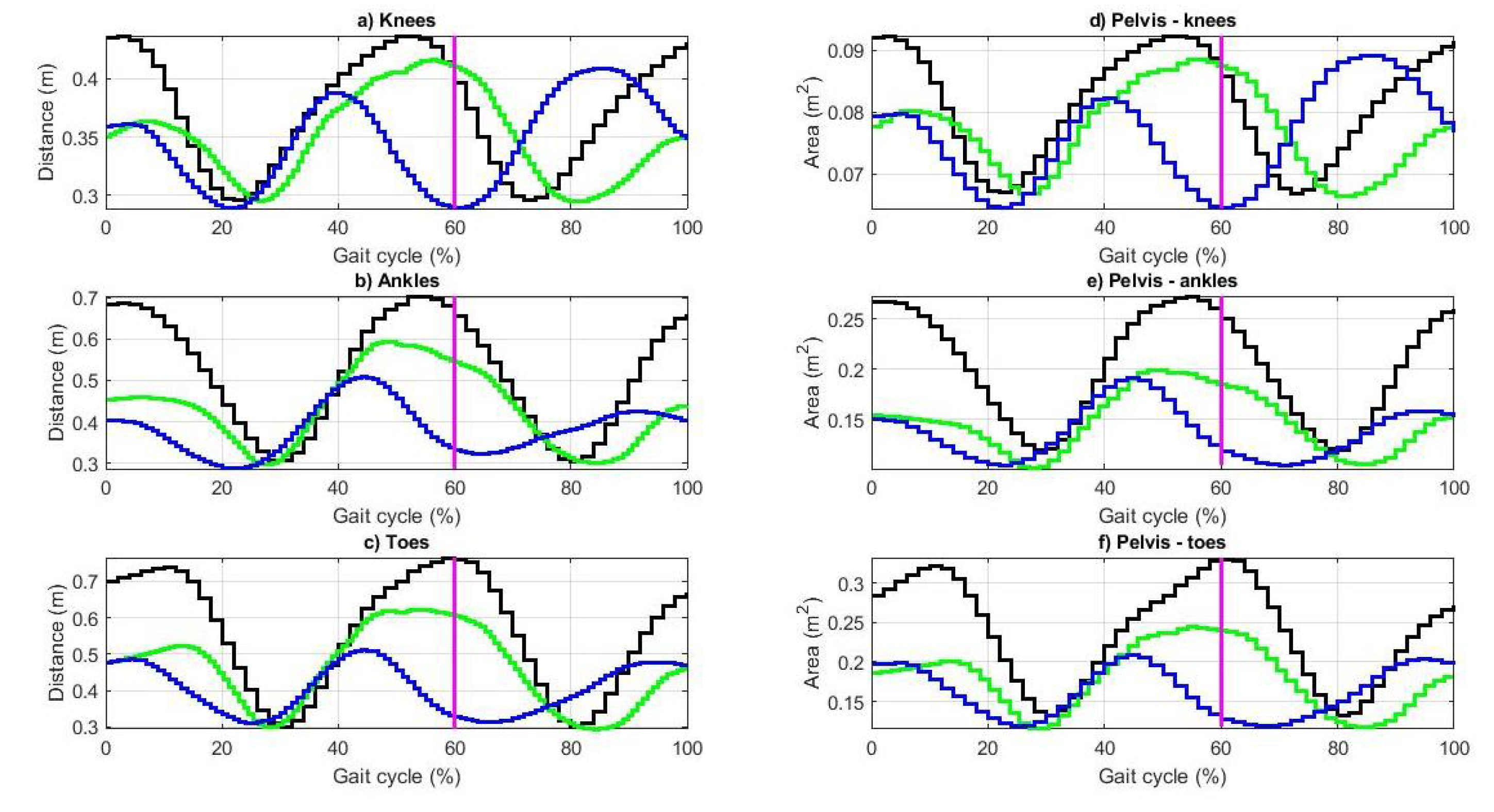
2.1.3. Parameters of Workspace for Gait Analysis

Gait analysis based on kinematics and kinetic modeling is widely used in clinical settings. However, full gait analysis is time-consuming and expensive [46]. While most of the systems used for measuring spatio-temporal gait parameters provide useful information, many of these only allow for local analysis. For this reason, in this work we propose non-common metrics on the gait space for global assessment. In robotics, as well as other disciplines, the Euclidean distance is the most common metric used in the Cartesian space to assess performance. However, it has not been used for gait analysis approaches. The Euclidean distance between the corresponding right and left joint reference frames (knees, ankles, and toes) of the lower limbs during walking can be calculated as
d Σ 2 R Σ 2 L 2 = m = 1 3 ( p m Σ 2 R p m Σ 2 L ) ,
d Σ 3 R Σ 3 L 2 = m = 1 3 ( p m Σ 3 R p m Σ 3 L ) ,
d Σ 4 R Σ 4 L 2 = m = 1 3 ( p m Σ 4 R p m Σ 4 L ) .
for the knees, ankles, and toes, respectively. Here, p m 1 Σ i , p m 2 Σ i , and p m 3 Σ i are the x, y, and z Cartesian coordinates of each joint reference. In the same way, in robotics the workspace is important in order to determine the facilities and operative needs. If we consider the gait workspace for each pair of joints as the area between the pelvic frame Σ 0 and both the right and left frame joint references (Figure 3), it is possible to establish this area as an objective metric. The Cartesian position in the workspace of the joint frame references (knees, ankles, and toes) of both lower limbs change depending on whether the gait is normal or abnormal (mild or severe crouch gaits). The area of the triangle formed by both references and the global frame can be used as a performance metric. That is, the degree of abnormality with respect to the normal gait pattern is seen in the decrease in the value of the area. These three areas allow a global analysis for each of these, or as a whole, globally for the entire kinematic chain. This approach can be very useful in either the diagnosis or the rehabilitation stage. The triangular areas during each gait phase are provided by
A P K = 1 2 Σ 2 R × Σ 2 L
for the knees, where ( Σ 0 ) is the origin of the frame vectors,
A P A = 1 2 Σ 3 R × Σ 3 L
for the ankles, and
A P T = 1 2 Σ 4 R × Σ 4 L
for the toes.
Generally, as mentioned in the previous section, gait analysis is carried out in the joint space, and when analysis is developed, only in the Cartesian space. This implies that a local analysis is performed for each of the lower limbs. In this work, we aim to propose statistical metrics such as the RMS value of the triangular areas in order to obtain a global evaluation of the performance of the eight-DoF kinematic chain based on metrics during a gait cycle. If the percentage of the gait cycle when each phase and event is evaluated, any of the metrics proposed in the Cartesian space are useful for comparing gaits in different stages. The Root Mean Square (RMS) value for each signal of the triangular areas is calculated as
A R M S = 1 M n = 1 N A T 2
where M is the total number of samples taken during the gait cycle and A T are the areas calculated in Equations (23)–(25). In the same sense, to obtain a global gait assessment, we concentrate the total area through the centroid of each triplet of triangles as well as a global centroid of these three triangles using the computational method of averaging Cartesian coordinates.

2.2. Gait Inverse Kinematics

Using the same skeletal model as for forward kinematics (Figure 2) [13], we calculate the gait inverse kinematics to obtain the joint coordinates q i , where i = 1 , 2 , ( 3 , 4 , 5 ) R , ( 3 , 4 , 5 ) L . We assume that the joint Cartesian coordinates concerning the global fixed frame Σ 0 are given. In addition, the lengths of the rigid-body segments l i are given. These coordinates could be obtained using a motion capture system with rigid markers in the joint references [14,47].
Initially, from Figure 4, the right hip is used as a reference and the rotation q 1 and list q 2 angles of the pelvis using Cartesian coordinates to perform spherical transformation, calculated as follows:
q 1 = a t a n 2 ( Σ 1 R x , Σ 1 R z ) ,
q 2 = sin 1 Σ 1 R y Σ 1 R x 2 + Σ 1 R y 2 + Σ 1 R z 2 .
In the same way, both q 1 and q 2 angles can be obtained from Figure 5.
Then, as the Cartesian coordinates for the hips, knees, ankles, and toes are given with respect the global fixed frame Σ 0 , an inverse homogeneous transformation of coordinates is required. Now, the knees, ankles and, toes are referred to the Σ 1 R frame in the sagittal plane, as shown in Figure 6. In this way, q 3 R , q 4 R , and q 5 R can be obtained locally as follows.
Let
R x = 1 0 0 0 c 2 s 2 0 s 2 c 2
R y = c 1 0 s 1 0 1 0 s 1 0 c 1
The above are the rotation matrices over the x and y axis, respectively, where c = c o s ( ) and s = s i n ( ) . In this work, the rotation over the z axis is not considered, as it is not used in forward kinematics. However, the model could be extended to consider the pelvic tilt movement. The local coordinates of the knee, the ankle, and the toe with respect to Σ 1 R are
Σ 2 R = Σ 2 r x Σ 2 r y Σ 2 r z = ( R y R x ) T Σ 1 R x Σ 1 R y Σ 1 R z + ( R y R x ) T Σ 2 R x Σ 2 R y Σ 2 R z
Σ 3 R = Σ 3 r x Σ 3 r y Σ 3 r z = ( R y R x ) T Σ 1 R x Σ 1 R y Σ 1 R z + ( R y R x ) T Σ 3 R x Σ 3 R y Σ 3 R z
Σ 4 R = Σ 4 r x Σ 4 r y Σ 4 r z = ( R y R x ) T Σ 1 R x Σ 1 R y Σ 1 R z + ( R y R x ) T Σ 4 R x Σ 4 R y Σ 4 R z
Then, from Figure 6, using the cosine law over the triangle with vertices Σ 1 R , Σ 2 R , and Σ 3 R , the flexoextension angle of the right knee is
q 4 R = π + ρ
where
ρ R = cos 1 Σ 2 r x 2 + Σ 2 r y 2 l 1 R 2 l 2 R 2 2 l 1 R l 2 R .
Meanwhile, the flexoextension angle of the right hip q 3 R is provided by
q 3 R = a t a n 2 ( Σ 3 r x , Σ 3 r y ) + ζ R
where
ζ R = sin 1 l 3 R sin ( ρ R ) Σ 3 r x 2 + Σ 3 r y 2
Similarly, in the same way over the triangle with vertices Σ 2 r , Σ 3 r , and Σ 4 r , the right ankle dorsi/plantar flexion angle q 5 R can be obtained from
q 5 R = π 2 o R
where
o R = cos 1 ( Σ 4 r x Σ 2 r x ) 2 + ( Σ 4 r y Σ 2 r y ) 2 l 3 R 2 l 4 R 2 2 l 3 R l 4 R .
Finally, to calculate the joint angles of the hip, knee, and ankle of the left lower limb we use Figure 7 and a similar process to that described above. The position configurations of the kinematic chain in Figure 6 and Figure 7 are given arbitrarily.

Parameters on Joint Space for Gait Analysis

Most of the systems used for gait data acquisition measure spatiotemporal parameters such as speed, cadence, cycle time, step length, and stride length [46]. However, most of these parameters do not provide enough information on the kinematic aspect. Joint angles during the gait cycle can be considered as a mathematical function, therefore, they can be analyzed in both the frequency and time domain, or alternatively by using methods from information theory. Statistical features of the joint functions, such as the mean ( q ¯ ) , standard deviation ( q S T D ) , root mean square ( q R M S ) , and shape factor ( q S F ) , are calculated from
q ¯ = i = 1 M q i ,
q S T D = i = 1 N ( q i q i ¯ ) 2 M 1 ,
q R M S = 1 M i = 1 N | q i | 2 ,
q S F = q R M S 1 M i = 1 N | q i | .
where, q i is the joint function and M is its length.

2.3. Virtual Gait Visualization

Visual feedback during gait analysis and rehabilitation is currently very important, and its effectiveness is improving. For this reason, in this work we have developed a framework for gait 3D visualization using Maya Autodesk, which is shown in Figure 8.
The starting point of the visualization framework is the creation or modeling of the 3D-CAD human skeleton model. In this work, we use an open-access skeletal model [48]. As access and orientation of the model are required as well, the referred orientation can be carried out based on the model shown in Figure 2. The data input of the keyframes control is the joint angles obtained on the inverse kinematic method, which are stored as the joint angles dataset. However, due to the data features and need for access in an automatic way through scripting, a data editing and scripting process is required. Subsequently, the 3D gait animation for gait visualization is programmed through a timeline that contains the number of samples of each gait. The timeline of the gait animation is controlled by the keyframes. Finally, a visual comparison between the three gaits over the three anatomical planes is carried out in order to compare the seven events for each plane and each gear a manual selection of the snapshot corresponding to each percentage of the cycle, taking as reference the seven events of the gait cycle. The seven events with the respective elapsed percentage of the gait cycle are initial contact (IC, 0%), opposite toe off (OTO, 12%), heel rise (HR, 30%), opposite initial contact (OIC, 40%), and toe off (TO, 60%), belonging the stance phase, while the feet adjacent (FA, 75%), tibia vertical (TV, 85%), and initial contact (IC, 100%) are associated with the stance phase [2]. The right lower limb (blue feet) is the reference for the beginning and the end of the gait cycle.

3. Results

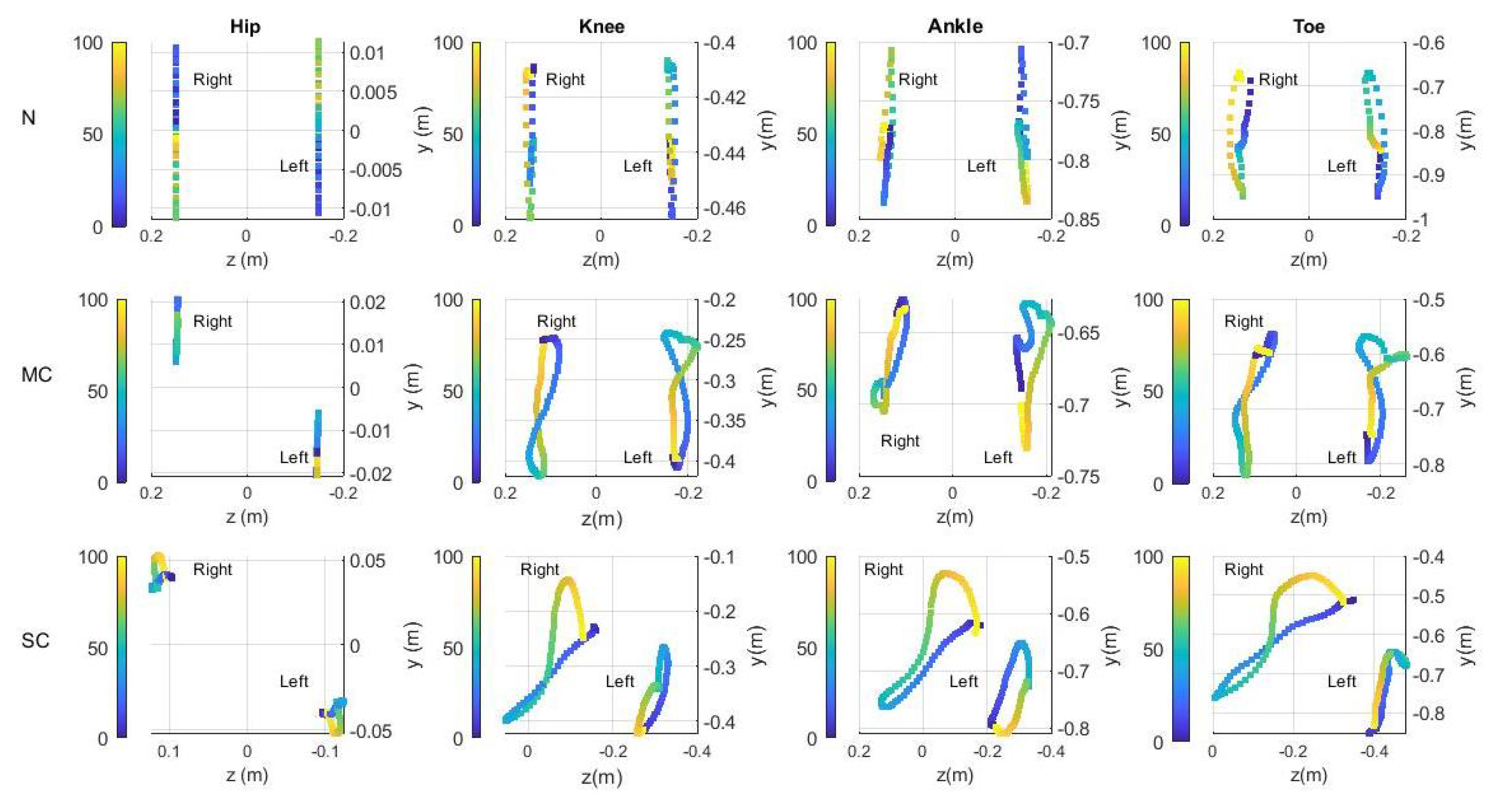
3.1. Gait Analysis on the Workspace

A visualization of the Cartesian coordinates of the reference frames of the model described in Section 2.1.2 are shown in Figure 9. The coordinates have been calculated using the joint angles of the dataset of the 2392- O p e n S i m model [49] as input in Equations (12)–(19). This model is well-known and widely used in biomechanical modeling settings; the experimental design used to obtain the gait data is presented in [50]. The number of samples ( M ) of the normal, mild crouch, and severe crouch gait signals are ( 51 ) , ( 119 ) , and Af ( 101 ) , respectively. These are the values used in this work to present the results using the gait cycle (%) as the reference. While the length of the eight rigid-body segments l 1 R , l 2 R , l 3 R , l 4 R , l 1 L , l 2 L , l 3 L , and l 4 L was adopted from [51], in this work, we aim at numerical validation for the proposed methods for forward and inverse kinematics using the widely used gait data. For this reason, we use only a single trial for each gait (normal, mild crouch, and severe crouch). However, it is possible to take difference gait trials as input.
The 4D plot shows a sagittal view of the right and left frame reference coordinates for gaits during a gait cycle: normal (N) in rows 1 and 2, mild crouch (MC) in rows 3 and 4, and severe crouch (SC) in rows 5 and 6 (Figure 9). In this work, we considered the global frame Σ 0 to be fixed, that is, gait analysis is similarly assumed on a treadmill. The color bar on the left side of the plots is related to the percentage of the elapsed gait cycle, and corresponds with one sample of the cycle in the plots.
In Figure 9, two main comparative approaches in the sagittal plane are shown. The comparison between lower limbs and the comparison of abnormal gaits were both performed by taking the normal gait pattern as the reference. In a normal gait, there is a correspondence between the coordinates of the right and left references; the difference is a phase shift of half a cycle from one to the other. For mild and severe crouch gaits, the same relationship as in the pattern does not occur. This allows for the establishment of the degree of severity between lower limbs. The same figure presents the workspace performance of the normal gait as the pattern. The pattern can be used to compare abnormal gaits based on both the joint workspace range and the shape factor. As mentioned in Section 1, most gait analysis works have reported only on the sagittal plane, because the analysis is focused on the hip, knee, and ankle joints. However, certain abnormalities related to pelvic movements, as well as global analysis, cannot be performed in the sagittal plane alone. For this reason, in this work we have extended the analysis to frontal plane (Figure 10) and transverse plane (Figure 11).
In the same way as the sagittal plane, the frontal plane allows us to visualize and compare the gait workspace performance between both lower limbs and different types of gaits together with the influence of the pelvic list, which is related to one of the lower limbs (in this case, the right one).
In Figure 12, the Euclidean distances between the frame references (knees, ankles, and toes) of both left and right limbs are shown. Equations (20)–(22) were used to calculate each sample of the gait cycle of each gait (N, MC, and SC).
The ranges of the Euclidian distance in a normal gait are 0.29 m d Σ 2 R Σ 2 L 0.43 m, 0.30 m d Σ 3 R Σ 3 L 0.68 m, and 0.29 m d Σ 4 R Σ 4 L 0.76 m for knees, ankles, and toes, respectively. Furthermore, Figure 12 shows the values of the triangular areas between the pelvis (base frame) and the joint reference frames (knees, ankles, and toes) (Section 2.1.3) of each gait trial, calculated by applying Equations (23)–(25). For the three triangles (Figure 3), the area for normal gait for each gait sample is greater than the areas in crouch gaits. For the three triangles in a normal gait, the ranges of the areas are 0.066 m 2 A P K 0.092 m 2 , 0.118 m 2 A P A 0.271 m 2 , and 0.113 m 2 A P T 0.332 m 2 . The maximum values of the areas in normal and mild crouch gait occur in the initial contact and the opposite contact events, while a severe crouch gait does not occur in the same events. This could be useful for relating the problem to the stage of the gait cycle. Table 1 presents a summary of the arithmetic mean, standard deviation, and root mean square level for both the distance and area metrics.
In Table 1, the value that best reflects the difference between the gaits for the six metric values is the arithmetic mean, closely followed by the RMS value, with the less significant for this purpose being the standard deviation. In a gait data analytics approach, it is possible to choose the most useful metric during the feature selection stage. In addition, all the results presented in this work are based only on one gait cycle, which is enough for the analysis, as the gait cycle can be considered a quasiperiodic signal. Although the assessment of the Euclidean distances and triangular areas are useful only for local analysis, the centroid of each of the areas and the total centroid used to obtain a metric of the location of the geometric center of the kinematic chain are useful in performing a global analysis. In Figure 13, frontal and transverse views of the global centroid for the three triangles of the normal gait adn mild and severe crouch gaits are shown. The plots in the same figure establish the range of workspace of a normal gait that can be used to assess abnormal gaits.

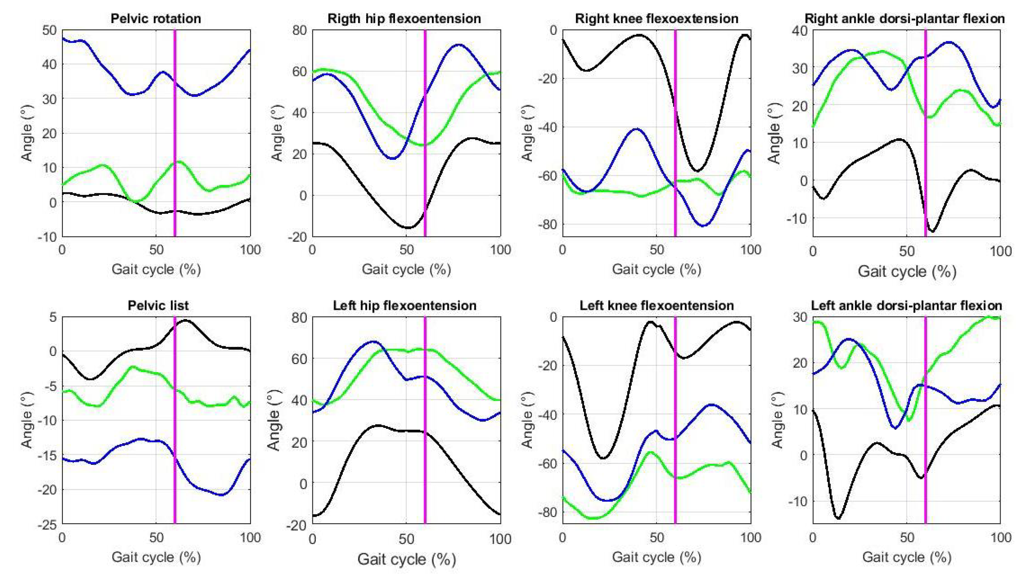
3.2. Gait Analysis on the Joint Space

Using the Cartesian coordinates calculated for each gait sample of normal gait and mild and severe crouch gaits with the proposed forward kinematics method (see Figure 1) as input in Equations (4)–(19), the joint angles of the eight degrees of freedom were calculated. However, Cartesian coordinates could be obtained from a Motion Capture (MoCap) system as well. Figure 14 shows the joint angle signals for the movements of pelvic rotation, pelvic list, hip and knee flexoextension, and ankle dorsi/plantar flexion of both the left and right lower limbs. For the normal gait, considering the right lower limb as the reference [2], the joint angles of the left lower limb are out of phase by half a cycle
Table 2 shows the minimum (Min) and maximum (Max) values of the range of motion (ROM) for each joint angle (Figure 14). From these values, the ROM of the normal gait is established as the gait pattern of reference. Then, gait analysis in the joint space is supported systematically and numerically by this pattern to determine abnormal gaits such as crouch gaits.
To objectively compare the normal gait and mild and severe crouch gaits in the anatomical space, statistical metrics were calculated. The arithmetic mean q ¯ , standard deviation q S T D , root mean square ( q R M S ) , and shape factor ( q S F ) values of the joint angles are shown in Table 3.
Table 3 provides quantitative information on the gait performance over the anatomical space, which can be used for local and global analysis. Considering the arithmetic mean as the metric for analysis, the statistically significant difference between the three gaits is established, which allows abnormal behaviors regarding the gait pattern to be classified and the degree of abnormality to be determined. In addition, in a normal gait, the arithmetic mean of the joint angles of both lower limbs are equal, qw the difference between the two is only offset by half a cycle. However, mild and severe crouch gaits are not the same. From the mean values, it is observed that the lower limbs do not have similar performance between them with respect to the gait pattern. Thus, it is possible to determine the degree of abnormality for each lower limb with respect to both each other and the overall pattern.
The standard deviation for the pelvis rotation angle q 1 is greater in severe crouch gait than in normal and mild crouch gaits. In both crouch gaits, the q S T D value of hip flexoextension is higher in the right joint than in the left one, which indicates a greater abnormality in the left hip. In both knee flexoextension and ankle dorsi/plantar flexion, the abnormalities occur in both joints, being more severe in mild crouch gaits. Regarding the RMS value in Table 3, both q 1 and q 2 have higher values for mild and severe crouch gaits than the gait pattern.
Although the arithmetic mean, standard deviation, and RMS level allow for the establishment of objective metrics to assess abnormal gaits regarding gait patterns, the signal shape factor is a novel metric for gait analysis based on the waveform of the joint angle signals. Table 3 shows no statistical difference for the SF values over the full cycle. However, it could be used locally in different phases of the gait cycle. It is necessary to focus both locally and globally on the other metrics. The data provided in Table 1, Table 2 and Table 3 describe accurate information for gait analysis. However, these are for a single gait signal, which allows manual data analysis. GA for multiple gaits involves high temporary, computationally, and specialty costs, which can lead to errors and requires subjective assessment by a specialist. Therefore, for automatic analysis for multidimensional, multi-variable, and large gait data, an approach based on machine learning can be used.

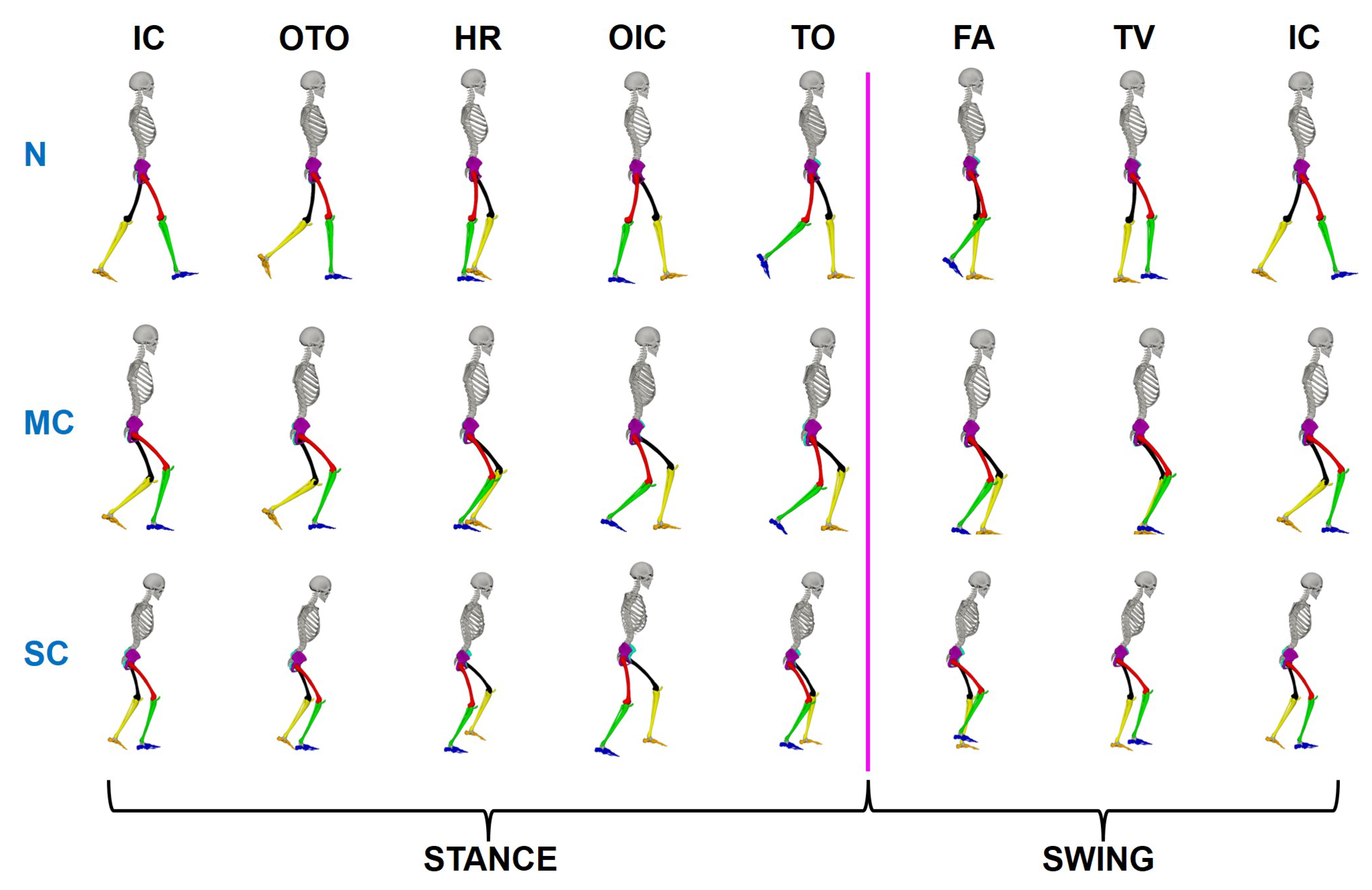
3.3. Virtual Gait Visualization

After the joint angles have been calculated using the inverse kinematics method proposed in this work, the angles are used as input for the 3D gait animation unit of the research framework presented in Section 2.3. Figure 15, Figure 16 and Figure 17 show a comparison of the stance and swing phases (seven events) of a gait cycle for normal, mild, and severe crouch gaits. Figure 15 shows a sagittal view of three gait performances, where excessive hip and knee flexoextension and ankle dorsi/plantar flexion is evident in crouch gaits. However, in order to obtain a global analysis the frontal and transverse planes views are useful, and are presented in Figure 16 and Figure 17, respectively.

4. Discussion

Gait analysis is commonly developed in the anatomical space, and the works presented in the workspace have generally been developed in the sagittal plane [14,15,34,35,36,37,38,39]. However, the information available in the frontal and transverse planes, mainly as regards pelvic movements, is very useful. Our findings allow for the determination that assessments in the Cartesian frontal and transverse planes are significant in determining gait abnormalities related to pelvic movements. In this sense, it is possible to develop an assessment for each of the lower limbs or for both together. In addition, the instrumentation advantages of acquiring and analyzing gait data in the gait space can reduce the need for invasive approaches and improve non-invasive ones.
The gait inverse kinematic method for gait analysis and visualization to solve the inverse kinematics of the eight-DoF lower limb model is useful for obtaining the joint angle references from the Cartesian coordinates. This approach could be used for vision-based system perception. The reduction in the calculation, computational complexity, and instrumentation required for data acquisition in the workspace is another advantage. The comparison between mild and severe crouch gaits using the normal gait as a reference is carried out in the anatomical space, achieving closer results than in workspace analysis. Gait analysis can be improved using metrics such as the arithmetic mean, standard deviation, RMS value, and shape factor to quantify and assess joint performance during walking. However, the manual data analysis developed in this work is commonly performed by a specialist, and represents high temporal and economic costs. This approach leads to bias and assessment errors, making necessary the application of artificial intelligence tools.
Visualization for abnormal crouched gaits using the normal gait pattern in the three anatomical planes as a reference provides a powerful bio-feedback tool. In an exergaming approach, gait visualization based on animation tools increases the success of the rehabilitation process for both the patient and the specialist. The versatility and performance of virtual environment modeling related to exergaming can be used to represent the user through an avatar and virtually modify the terrain context. The impact on a patient’s emotions through kinesthetic perception during rehabilitation represents a useful stimulus during rehabilitation tasks. In addition, the advantages of developing a visualization framework in Autodesk Maya make it possible to visualize in real-time any patient that is not already in the database, automatically adjusting to the subject’s anthropometry.

5. Conclusions

This paper presents a gait forward and inverse kinematics framework for modeling gait during walking for analysis and visualization purposes. Both methods are used to model an eight-DoF kinematic chain representing the lower limbs during the gait cycle. In addition, gait workspace and gait anatomical space analysis allows for establishing the normal gait ranges as the pattern to assess gait using objective metrics. We present an extended assessment for mild and severe crouch gaits in both the workspace and the anatomical space using statistical metrics, with the normal gait used as a reference. Depending on whether the aim of the analysis is diagnostic or rehabilitation assessment, any of these metrics could be used to classify gaits. The advantages of the proposed forward kinematics method using quaternions algebra is that is it scalable and useful for modeling kinematic chains, increasing the degrees of freedom, and avoiding gimbal lock and mathematical complexity. Reduction in mathematical and computational complexity as well as in the instrumentation required for data acquisition in the workspace is one of the main advantages of the approach for gait inverse kinematics presented here.
A graphical comparison using the gait visualization framework for the seven events of the gait cycle for normal, mild, and severe crouch gaits was carried out. This is an important aspect for improving interpretation by specialists as well as the motivation of patients. The advantages of modeling and visualization following the approach proposed in this work as a future perspective offers an alternative approach to the development of a comprehensive exergaming rehabilitation platform. In addition, both virtual gait visualization feedback in real time for any patient and the anthropometry of the subject can be adjusted automatically.
In future work, we intend to develop a three-DoF experimental platform to emulate and assess the gait cycle for different gaits in the sagittal plane. In addition, we plan to acquire the Cartesian coordinates for the eight degrees of freedom with a MoCap system for investigating real patients. Ultimately, we intend to develop a gait recognition framework based on the biomechanical modeling and metrics established in this paper.

Author Contributions

Conceptualization, J.-C.G.-I. and O.-A.D.-R.; methodology, J.-C.G.-I., O.-A.D.-R. and O.L.-O.; software, J.-C.G.-I. and O.-A.D.-R.; validation, O.-A.D.-R., O.L.-O. and J.-P.O.-O.; formal analysis, J.P.-R. and F.M.-G.; investigation, O.-A.D.-R.; resources, O.-A.D.-R.; data curation, J.-C.G.-I.; writing—original draft preparation, J.-C.G.-I. and O.-A.D.-R.; writing—review and editing, J.P.-R., J.-P.O.-O. and F.M.-G.; visualization, J.-C.G.-I., O.-A.D.-R. and O.L.-O. All authors have read and agreed to the published version of the manuscript.

Funding

This research received no external funding.

Institutional Review Board Statement

Not applicable.

Informed Consent Statement

Not applicable.

Data Availability Statement

Data available on request.

Acknowledgments

The first author is grateful to CONACyT for granting the scholarship with application number: 2022-000002-01NACF-07659. The second author thanks to the research direction of the Autonomous University of the State of Hidalgo.

Conflicts of Interest

The authors declare no conflict of interest.

References

  1. Stergiou, N. Biomechanics and Gait Analysis; Academic Press: Cambridge, MA, USA, 2020. [Google Scholar]
  2. Whittle, M.W. Gait Analysis: An Introduction; Butterworth-Heinemann: Oxford, UK, 2014. [Google Scholar]
  3. Beaulieu, M.L.; Lamontagne, M.; Beaulé, P.E. Lower limb biomechanics during gait do not return to normal following total hip arthroplasty. Gait Posture 2010, 32, 269–273. [Google Scholar] [CrossRef]
  4. Ogihara, H.; Tsushima, E.; Kamo, T.; Sato, T.; Matsushima, A.; Niioka, Y.; Asahi, R.; Azami, M. Kinematic gait asymmetry assessment using joint angle data in patients with chronic stroke—A normalized cross-correlation approach. Gait Posture 2020, 80, 168–173. [Google Scholar] [CrossRef]
  5. Smith, M.C.; Stinear, J.; Stinear, C.M. The effects of unilateral step training and conventional treadmill training on gait asymmetry in patients with chronic stroke. Gait Posture 2021, 87, 156–162. [Google Scholar] [CrossRef]
  6. Kobsar, D.; Barden, J.M.; Clermont, C.; Wilson, J.; Ferber, R. Sex differences in the regularity and symmetry of gait in older adults with and without knee osteoarthritis. Gait Posture 2022, 95, e192–e197. [Google Scholar] [CrossRef]
  7. Munteanu, S.; Barton, C. Lower limb biomechanics during running in individuals with Achilles tendinopathy: A systematic review. J. Sci. Med. Sport 2010, 13, e74–e75. [Google Scholar] [CrossRef]
  8. Yamada, M.; Aoyama, T.; Mori, S.; Nishiguchi, S.; Okamoto, K.; Ito, T.; Muto, S.; Ishihara, T.; Yoshitomi, H.; Ito, H. Objective assessment of abnormal gait in patients with rheumatoid arthritis using a smartphone. Rheumatol. Int. 2012, 32, 3869–3874. [Google Scholar] [CrossRef]
  9. Chinn, L.; Dicharry, J.; Hart, J.M.; Saliba, S.; Wilder, R.; Hertel, J. Gait kinematics after taping in participants with chronic ankle instability. J. Athl. Train. 2014, 49, 322–330. [Google Scholar] [CrossRef] [Green Version]
  10. Saad, A.; Zaarour, I.; Guerin, F.; Bejjani, P.; Ayache, M.; Lefebvre, D. Detection of freezing of gait for Parkinson’s disease patients with multi-sensor device and Gaussian neural networks. Int. J. Mach. Learn. Cybern. 2017, 8, 941–954. [Google Scholar] [CrossRef]
  11. Xu, H.; Li, X.; Shi, Y.; An, L.; Taylor, D.; Christman, M.; Morse, J.; Merryweather, A. Hospital bed height influences biomechanics during bed egress: A comparative controlled study of patients with Parkinson disease. J. Biomech. 2021, 115, 110116. [Google Scholar] [CrossRef]
  12. Ramadoss, P.; Rapetti, L.; Tirupachuri, Y.; Grieco, R.; Milani, G.; Valli, E.; Dafarra, S.; Traversaro, S.; Pucci, D. Whole-Body Human Kinematics Estimation using Dynamical Inverse Kinematics and Contact-Aided Lie Group Kalman Filter. arXiv 2022, arXiv:2205.07835. [Google Scholar]
  13. Kainz, H.; Modenese, L.; Lloyd, D.; Maine, S.; Walsh, H.; Carty, C. Joint kinematic calculation based on clinical direct kinematic versus inverse kinematic gait models. J. Biomech. 2016, 49, 1658–1669. [Google Scholar] [CrossRef]
  14. Barki, A.; Kendricks, K.; Tuttle, R.F.; Bunker, D.J.; Borel, C.C. Extraction of human gait signatures: An inverse kinematic approach using Groebner basis theory applied to gait cycle analysis. In Proceedings of the Active and Passive Signatures IV; SPIE: Bellingham, WA, USA, 2013; Volume 8734, pp. 138–151. [Google Scholar]
  15. Parent, A.; Pouliot-Laforte, A.; Dal Maso, F.; Cherni, Y.; Marois, P.; Ballaz, L. Muscle fatigue during a short walking exercise in children with cerebral palsy who walk in a crouch gait. Gait Posture 2019, 72, 22–27. [Google Scholar] [CrossRef]
  16. Dussault-Picard, C.; Mohammadyari, S.; Arvisais, D.; Robert, M.; Dixon, P. Gait adaptations of individuals with cerebral palsy on irregular surfaces: A Scoping Review. Gait Posture 2022, 96, 35–46. [Google Scholar] [CrossRef]
  17. Rethlefsen, S.A.; Blumstein, G.; Kay, R.M.; Dorey, F.; Wren, T.A. Prevalence of specific gait abnormalities in children with cerebral palsy revisited: Influence of age, prior surgery, and Gross Motor Function Classification System level. Dev. Med. Child Neurol. 2017, 59, 79–88. [Google Scholar] [CrossRef]
  18. Cho, S.; Lee, K.D.; Park, H.S. A Mobile Cable-Tensioning Platform to Improve Crouch Gait in Children With Cerebral Palsy. IEEE Trans. Neural Syst. Rehabil. Eng. 2022, 30, 1092–1102. [Google Scholar] [CrossRef]
  19. Lerner, Z.F.; Damiano, D.L.; Park, H.S.; Gravunder, A.J.; Bulea, T.C. A robotic exoskeleton for treatment of crouch gait in children with cerebral palsy: Design and initial application. IEEE Trans. Neural Syst. Rehabil. Eng. 2016, 25, 650–659. [Google Scholar] [CrossRef]
  20. Adil, S.; Al Jumaily, A.; Anam, K. AW-ELM-based Crouch Gait recognition after ischemic stroke. In Proceedings of the 2016 5th International Conference on Electronic Devices, Systems and Applications (ICEDSA), Ras Al Khaimah, United Arab Emirates, 6–8 December 2016; IEEE: Piscataway, NJ, USA, 2016; pp. 1–4. [Google Scholar]
  21. Jahnsen, R.; Villien, L.; Aamodt, G.; Stanghelle, J.; Holm, I. Musculoskeletal pain in adults with cerebral palsy compared with the general population. J. Rehabil. Med. 2004, 36, 78–84. [Google Scholar] [CrossRef] [Green Version]
  22. Opheim, A.; Jahnsen, R.; Olsson, E.; Stanghelle, J.K. Walking function, pain, and fatigue in adults with cerebral palsy: A 7-year follow-up study. Dev. Med. Child Neurol. 2009, 51, 381–388. [Google Scholar] [CrossRef]
  23. Rose, J.; Gamble, J.G.; Burgos, A.; Medeiros, J.; Haskell, W.L. Energy expenditure index of walking for normal children and for children with cerebral palsy. Dev. Med. Child Neurol. 1990, 32, 333–340. [Google Scholar] [CrossRef]
  24. O’Sullivan, R.; Marron, A.; Brady, K. Crouch gait or flexed-knee gait in cerebral palsy: Is there a difference? A systematic review. Gait Posture 2020, 82, 153–160. [Google Scholar] [CrossRef]
  25. Spong, M.W.; Vidyasagar, M. Robot Dynamics and Control; John Wiley & Sons: Hoboken, NJ, USA, 2008. [Google Scholar]
  26. Ho, T.; Kang, C.G.; Lee, S. Efficient closed-form solution of inverse kinematics for a specific six-DOF arm. Int. J. Control. Autom. Syst. 2012, 10, 567–573. [Google Scholar] [CrossRef]
  27. Kucuk, S.; Bingul, Z. Inverse kinematics solutions for industrial robot manipulators with offset wrists. Appl. Math. Model. 2014, 38, 1983–1999. [Google Scholar] [CrossRef]
  28. Dulęba, I.; Opałka, M. A comparison of Jacobian-based methods of inverse kinematics for serial robot manipulators. Int. J. Appl. Math. Comput. Sci. 2013, 23, 373–382. [Google Scholar] [CrossRef] [Green Version]
  29. Di Vito, D.; Natale, C.; Antonelli, G. A comparison of damped least squares algorithms for inverse kinematics of robot manipulators. IFAC-PapersOnLine 2017, 50, 6869–6874. [Google Scholar] [CrossRef]
  30. Hamilton, W. First Motive for naming the Quotient of two Vectors a Quaternion. Elem. Quaternions 1866, 110–113. [Google Scholar]
  31. Cohen, A.; Shoham, M. Hyper Dual Quaternions representation of rigid bodies kinematics. Mech. Mach. Theory 2020, 150, 103861. [Google Scholar] [CrossRef]
  32. Özgür, E.; Mezouar, Y. Kinematic modeling and control of a robot arm using unit dual quaternions. Robot. Auton. Syst. 2016, 77, 66–73. [Google Scholar] [CrossRef]
  33. Baker, R.; Leboeuf, F.; Reay, J.; Sangeux, M. The conventional gait model-success and limitations. Handb. Hum. Motion 2018, 489–508. [Google Scholar]
  34. Lin, C.J.; Guo, L.Y.; Su, F.C.; Chou, Y.L.; Cherng, R.J. Common abnormal kinetic patterns of the knee in gait in spastic diplegia of cerebral palsy. Gait Posture 2000, 11, 224–232. [Google Scholar] [CrossRef]
  35. Rodda, J.; Graham, H.K.; Nattrass, G.; Galea, M.P.; Baker, R.; Wolfe, R. Correction of severe crouch gait in patients with spastic diplegia with use of multilevel orthopaedic surgery. JBJS 2006, 88, 2653–2664. [Google Scholar] [CrossRef]
  36. Steele, K.M.; Seth, A.; Hicks, J.L.; Schwartz, M.S.; Delp, S.L. Muscle contributions to support and progression during single-limb stance in crouch gait. J. Biomech. 2010, 43, 2099–2105. [Google Scholar] [CrossRef] [Green Version]
  37. Hu, X.; Soh, G.S. A study on estimation of planar gait kinematics using minimal inertial measurement units and inverse kinematics. In Proceedings of the 2014 36th Annual International Conference of the IEEE Engineering in Medicine and Biology Society, Chicago, IL, USA, 26–30 August 2014; IEEE: Piscataway, NJ, USA, 2014; pp. 6911–6914. [Google Scholar]
  38. Roy, G.; Mukherjee, S.; Das, T.; Bhaumik, S. Single Support Phase Gait Kinematics and Kinetics for a Humanoid Lower Limb Exoskeleton. In Proceedings of the 2020 IEEE Region 10 Symposium (TENSYMP), Dhaka, Bangladesh, 5–7 June 2020; IEEE: Piscataway, NJ, USA, 2020; pp. 138–141. [Google Scholar]
  39. Catelli, D.S.; Cotter, B.; Lamontagne, M.; Grammatopoulos, G. Spine, Pelvis and Hip Kinematics—Characterizing the Axial Plane in Healthy and Osteoarthritic Hips. Appl. Sci. 2021, 11, 9921. [Google Scholar] [CrossRef]
  40. Surer, E.; Kose, A. Methods and technologies for gait analysis. In Computer Analysis of Human Behavior; Springer: Berlin/Heidelberg, Germany, 2011; pp. 105–123. [Google Scholar]
  41. Bethi, S.R. Exergames for telerehabilitation. arXiv 2020, arXiv:2006.10110. [Google Scholar]
  42. Thikey, H.; van Wjick, F.; Grealy, M.; Rowe, P. A need for meaningful visual feedback of lower extremity function after stroke. In Proceedings of the 2011 5th International Conference on Pervasive Computing Technologies for Healthcare (PervasiveHealth) and Workshops, Dublin, Ireland, 23–26 May 2011; IEEE: Piscataway, NJ, USA, 2011; pp. 379–383. [Google Scholar]
  43. Uzor, S.; Baillie, L. Recov-R: Evaluation of a home-based tailored exergame system to reduce fall risk in seniors. ACM Trans. Comput.-Hum. Interact. (TOCHI) 2019, 26, 1–38. [Google Scholar] [CrossRef]
  44. Pacheco, T.B.F.; de Medeiros, C.S.P.; de Oliveira, V.H.B.; Vieira, E.R.; De Cavalcanti, F. Effectiveness of exergames for improving mobility and balance in older adults: A systematic review and meta-analysis. Syst. Rev. 2020, 9, 1–14. [Google Scholar] [CrossRef]
  45. Cardenas, A.; Warner, D.; Switzer, L.; Graham, T.N.; Cimolino, G.; Fehlings, D. Inpatient Exergames for Children with Cerebral Palsy following Lower Extremity Orthopedic Surgery: A Feasibility Study. Dev. Neurorehabilit. 2021, 24, 230–236. [Google Scholar] [CrossRef]
  46. Veilleux, L.N.; Raison, M.; Rauch, F.; Robert, M.; Ballaz, L. Agreement of spatio-temporal gait parameters between a vertical ground reaction force decomposition algorithm and a motion capture system. Gait Posture 2016, 43, 257–264. [Google Scholar] [CrossRef]
  47. Filtjens, B.; Ginis, P.; Nieuwboer, A.; Slaets, P.; Vanrumste, B. Automated freezing of gait assessment with marker-based motion capture and multi-stage spatial-temporal graph convolutional neural networks. J. Neuroeng. Rehabil. 2022, 19, 1–14. [Google Scholar] [CrossRef]
  48. Gumroad. Skeleton Maya Rig, 2022. Available online: https://truongcgartist.gumroad.com/l/bdbxF (accessed on 30 May 2022).
  49. Seth, A.; Hicks, J.L.; Uchida, T.K.; Habib, A.; Dembia, C.L.; Dunne, J.J.; Ong, C.F.; DeMers, M.S.; Rajagopal, A.; Millard, M.; et al. OpenSim: Simulating musculoskeletal dynamics and neuromuscular control to study human and animal movement. PLoS Comput. Biol. 2018, 14, e1006223. [Google Scholar] [CrossRef] [Green Version]
  50. John, C.T.; Seth, A.; Schwartz, M.H.; Delp, S.L. Contributions of muscles to mediolateral ground reaction force over a range of walking speeds. J. Biomech. 2012, 45, 2438–2443. [Google Scholar] [CrossRef] [Green Version]
  51. Tadano, S.; Takeda, R.; Miyagawa, H. Three dimensional gait analysis using wearable acceleration and gyro sensors based on quaternion calculations. Sensors 2013, 13, 9321–9343. [Google Scholar] [CrossRef] [PubMed]
Figure 1. Research framework for gait forward and inverse kinematics analysis and visualization.
Applsci 12 10197 g001
Figure 2. Eight-DoF open kinematic chain used to model the lower limbs during gait.
Applsci 12 10197 g002
Figure 3. Representation for calculating triangle gait workspace areas between pelvis and joint references: (a) pelvis–knees, (b) pelvis–ankles and (c) pelvis–toes.
Applsci 12 10197 g003
Figure 4. Right hip reference used to obtain the rotation and list angles of the pelvis.
Applsci 12 10197 g004
Figure 5. Left hip reference used to obtain the rotation and list angles of the pelvis.
Applsci 12 10197 g005
Figure 6. Right hip–knee–ankle–toe kinematic chain used to obtain q 3 R , q 4 R , and q 5 R .
Applsci 12 10197 g006
Figure 7. Left hip–knee–ankle–toe kinematic chain used to obtain q 3 L , q 4 L and q 5 L .
Applsci 12 10197 g007
Figure 8. 3D virtual gait visualization framework.
Applsci 12 10197 g008
Figure 9. Sagittal plane view of the Cartesian coordinates of hip, knee, ankle, and toe of both right and left lower limbs during a gait cycle. For normal gait (N), rows 1 and 2; for mild crouch gait (MC), rows 3 and 4; and for severe crouch gait (SC), rows 5 and 6. Columns 1, 2, 3, and 4 plot the hip, knee, ankle, and toe, respectively.
Applsci 12 10197 g009
Figure 10. Frontal plane view of the Cartesian coordinates of hip, knee, ankle, and toe of both right and left lower limbs during a gait cycle. For normal gait (N), row 1; for mild crouch gait (MC), row 2; and for severe crouch gait (SC), row 3. Columns 1, 2, 3, and 4 are used to plot the hip, knee, ankle, and toe, respectively.
Applsci 12 10197 g010
Figure 11. Transverse plane view of the Cartesian coordinates of hip, knee, ankle, and toe of both right and left lower limbs during a gait cycle. For normal gait (N), row 1; for mild crouch gait (MC), row 2; and for severe crouch gait (SC), row 3. Columns 1, 2, 3, and 4 are used to plot hip, knee, ankle, and toe, respectively.
Applsci 12 10197 g011
Figure 12. Euclidian distances between reference frames of both lower limbs (a) knees, (b) ankles, and (c) toes. Triangular areas between pelvis (base frame) and joint references of both lower limbs (d) knees, (e) ankles, and (f) toes for normal gait (black), mild crouch gait (green), and severe crouch gait (blue) during a gait cycle. The magenta vertical line represents the end of the stance phase.
Applsci 12 10197 g012
Figure 13. Sagittal, frontal, and transverse views of the global centroids of the triangles between joint references for a cycle of normal, mild crouch, and severe crouch gait cycles.
Applsci 12 10197 g013
Figure 14. Joint angles for pelvic rotation ( q 1 ), pelvic list ( q 2 ), hip flexoextension ( q 3 ), knee flexoextension ( q 4 ), and ankle dorsi/plantar flexion of the lower limbs for normal gait (black), mild crouch gait (green), and severe crouch gait (blue). The vertical line (magenta) represents the end of the stance phase.
Applsci 12 10197 g014
Figure 15. Sagittal plane view of the 3D gait animation of normal gait (N), mild crouch gait (MC), and severe crouch gait (SC) in the seven events of the two phases of the gait cycle. The magenta vertical line represents the end of the stance phase.
Applsci 12 10197 g015
Figure 16. Frontal plane view of the 3D gait animation of normal (N), mild crouch (MC), and severe crouch (SC) gaits in the seven events of the two phases of the gait cycle. The magenta vertical line represents the end of the stance phase.
Applsci 12 10197 g016
Figure 17. Lower transverse view of the 3D gait animation of normal gait (N), mild crouch gait (MC), and severe crouch gait (SC) in the seven events of the gait cycle.
Applsci 12 10197 g017
Table 1. Statistical measures for Euclidean distances and triangular areas of joint reference frames: Arithmetic Mean (MEAN), Standard Deviation (STD), and Root Mean Square value (RMS) for normal (N), mild crouch (MC), and severe crouch (SC) gaits.
Normal (N)Mild Crouch (MC)Severe Crouch (SC)
METRICMEANSTDRMSMEANSTDRMSMEANSTDRMS
d Σ 2 R Σ 2 L (m)0.3730.0490.3760.3500.0380.3520.3460.0380.348
d Σ 3 R Σ 3 L (m)0.5200.1380.5380.4320.0920.4410.3810.0580.386
d Σ 4 R Σ 4 L (m)0.5630.1570.5840.4590.1070.4710.4050.0660.410
A P K (m 2 )0.0810.0080.080.0770.0070.0770.0760.0070.076
A P A (m 2 )0.2030.0530.2090.1470.0300.1500.1360.0250.138
A P T (m 2 )0.2390.0650.2480.1780.0410.1830.1610.0310.164
Table 2. Range of motion (ROM) of the joint angles of each movement of the eight-DoF inverse kinematic model based on Figure 14.
Normal (N)Mild Crouch (MC)Severe Crouch (SC)
JA Min ( o ) Max ( o ) Min ( o ) Max ( o ) Min ( o ) Max ( o )
q 1 −3.5762.5600.02011.61730.7847.611
q 2 −4.0974.413−8.047−2.270−20.783−12.690
q 3 R −15.92127.41823.99260.63317.48872.673
q 3 L −15.89727.41937.45564.15329.94267.872
q 4 R −58.234−2.270−68.687−58.242−80.684−40.947
q 4 L −58.207−2.271−82.737−55.463−75.453−36.203
q 5 R −13.78510.74113.79834.15119.18736.610
q 5 L −13.91910.7497.34529.9215.69225.056
Table 3. Arithmetic mean q ¯ , standard deviation q S T D , root mean square level ( q R M S ) , and shape factor ( q S F ) values for gait analysis in the anatomical space considering Figure 14.
Normal (N)Mild Crouch (MC)Severe Crouch (SC)
JA q ¯ ( o ) q STD ( o ) q RMS ( o ) q SF ( o ) q ¯ ( o ) q STD ( o ) q RMS ( o ) q SF ( o ) q ¯ ( o ) q STD ( o ) q RMS ( o ) q SF ( o )
q 1 −0.652.292.351.106.273.177.021.1237.105.3337.471.01
q 2 0.222.332.311.29−5.971.886.251.04−16.202.6516.411.01
q 3 R 9.7115.6818.311.1244.4213.4246.391.0448.5316.9751.391.06
q 3 L 9.7115.6618.291.1252.959.9153.871.0247.1612.1748.691.03
q 4 R −19.9818.3126.981.35−64.852.7964.911.00−60.7111.2261.731.02
q 4 L −19.9818.3026.971.35−68.328.4868.841.01−54.0612.7655.531.02
q 5 R 1.156.396.421.2524.666.5125.490.3929.814.8230.191.01
q 5 L 1.126.426.461.2521.536.2022.401.0415.295.2016.141.05
Publisher’s Note: MDPI stays neutral with regard to jurisdictional claims in published maps and institutional affiliations.

