Article

IoT-Ready Temperature Probe for Smart Monitoring of Forest Roads

1
Research Centre, University of Zilina, Univerzitna 8215/1, 010 26 Zilina, Slovakia
2
Faculty of Materials Science and Technology, Slovak University of Technology, Jana Bottu 2781/25, 917 24 Trnava, Slovakia
3
TNtech, s.r.o., Lucna 1014/9, 014 01 Bytča, Slovakia
4
Faculty of Organization and Informatics, University of Zagreb, Pavlinska 2, 42000 Varazdin, Croatia
*
Authors to whom correspondence should be addressed.
Appl. Sci. 2022, 12(2), 743; https://doi.org/10.3390/app12020743
Submission received: 8 December 2021 / Revised: 5 January 2022 / Accepted: 9 January 2022 / Published: 12 January 2022
(This article belongs to the Special Issue Sustainable Agriculture and Advances of Remote Sensing)

Abstract

:
Currently, we are experiencing an ever-increasing demand for high-quality transportation in the distinctive natural environment of forest roads, which can be characterized by significant weather changes. The need for more effective management of the forest roads environment, a more direct, rapid response to fire interventions and, finally, the endeavor to expand recreational use of the woods in the growth of tourism are among the key factors. A thorough collection of diagnostic activities conducted on a regular basis, as well as a dataset of long-term monitored attributes of chosen sections, are the foundations of successful road infrastructure management. Our main contribution to this problem is the design of a probe for measuring the temperature profile for utilization in stand-alone systems or as a part of an IoT solution. We have addressed the design of the mechanical and electrical parts with emphasis on the accuracy of the sensor layout in the probe. Based on this design, we developed a simulation model, and compared the simulation results with the experimental results. An experimental installation was carried out which, based on measurements to date, confirmed the proposed probe meets the requirements of practice and will be deployed in a forest road environment.

1. Introduction

Forest roads are often considered a marginal point of interest within a country’s road infrastructure and a considerable number of academic articles are devoted to general transportation routes [1,2]. This fact is not wrong and does not need to be contradicted in the means of value for money. These allegations are based in particular on the volume and nature of the traffic that these roads must bear for a reasonable time period. Currently, there is, on the other hand, an ever-growing demand for high-quality mobility in this specific natural environment, which can be characterized by extreme fluctuations of weather conditions. The list of main reasons includes the requirement for more efficient management of the forest roads environment, a more straightforward, quick approach to fire interventions [3] and the final reason is in the effort for broader recreational utilization of the forests in the development of tourism. The conclusions of some studies are also interesting, such as [4], which points to the direct relationship between the quality of forest infrastructure and the economic value that can be obtained from forests. Not only for these reasons, but the authorities responsible are considerably concerned with ideas of implementing specific management procedures with a long-lasting effect into the process of forest road management. These procedures and systems based on them follow approaches applied within the generally available road networks. The basis of such applied instruments for effective management of road infrastructure, is a comprehensive set of diagnostic tasks regularly performed and a dataset of long-term monitored properties of selected sections [5,6]. The previously mentioned represents the simple starting point for the decision making on early construction interventions in the roads, either through a general routine maintenance, repairs, or reconstruction. At the same time, the information obtained by monitoring existing roads helps us to create new and improve existing standards associated with the comprehensive renewal and construction of new roads, taking into account the geospatial optimization of their situation and application of the innovative material composition as referred to in [7,8]. Within the concept of comprehensive monitoring and diagnostics, several measures need to be put in place. It is mainly a matter of regular data collection application of selected data from the forest road network, such as road bearing capacity, transverse and longitudinal unevenness and roughness. Measurements must be suitably accompanied by a network of stationary meteorological measuring stations at predefined road sections. Accomplishing this task will provide the required inputs for the correct evaluation of the collected data on the condition of the structure and the road surface. Such stations include special sensors evaluating the temperature profile of roads in both the vertical and horizontal directions, soil sensors installed in the immediate vicinity of the road, frost sensors, road pollution sensors and various additional meteorological sensors for use on the road network [9,10]. The data collected using these stations in combination with selected characteristics of the road condition obtained by diagnostics, might bring new results in the form of defining specific dependencies present within the specific road construction in the forest environment. As an application example, we can mention, e.g., determining the relationship between the bearing capacity of the subsoil and the climatic conditions in the forest environment, or determining the relationship between the influence of extreme climatic thermal effects on the road surface roughness. Their aim is, among other issues, to improve existing and conduct new degradation functions related to the life cycle of roads and to determine their residual life. For purposes related to comprehensive diagnostics and monitoring, it is required to design specially modified meteorological sets directly adapted to the tasks associated with the monitoring of forest roads. Several commercial products from reputable manufacturers are available on the market, most of which are intended for precisely defined uses. In our case, we decided to design our own solution that will be suitable for use in a forest environment. However, the proposed device can be used in other areas beyond the originally intended use. A suitable example us smart city solutions [11] and industrial automation solutions [12]. In this article, we focused our efforts on the first part of the joint work, which is the design and implementation of an IoT ready temperature probe for measuring the vertical temperature profile of the soil. Vertical heat transfer in the soil is an indicator of important properties of the soil and thus it is possible to indirectly observe physical events, such as heat transfer transferred by groundwater as an indicator of surface water at different depths [13]. From the hydrology point of view, it is possible to monitor the movement of water and the renewal of the water source through the rain. By creating a vertical temperature soil profile, it is also possible to monitor external atmospheric influences and other interventions in the environment, respectively. In addition to our area of interest in forest roads, it is possible to extend usage to other areas, e.g., agriculture, where the information on heat transfer and form of irrigation in the vertical direction is of significant value [14]. It is interesting to monitor temperature in the depth of plant roots, as plant roots are known to be stimulated to grow in warmer environments [15]. Monitoring of temperature profiles is commonly used, while several solutions of analog and digital temperature sensors are available. In [16], the authors address the issue of monitoring the temperature of the vertical and horizontal profile of the road surface using low-cost temperature sensors DS18B20 [17,18]. The purpose of monitoring the temperature profile [10] and logging the measured data was to investigate the freezing effect on the degradation of the road body in cold areas. The distribution of the measuring points of the vertical profile probe ranged from 30 mm to 4 m. They monitored one cycle of freezing and thawing of the subsoil and the effect of the change in atmospheric temperature on the individual monitored layers. In the article by Liu et al. [19], the authors monitored changes in soil temperature by application using LM35 temperature sensors, which needed to be calibrated for measurement purposes, due to the minor differences in the characteristics of individual sensors. The authors investigated the effect of using a paper cover film on the change and delay of the soil temperature at a depth of 100 mm depending on the change in outdoor temperature for agricultural purposes. However, in [9,13], the authors do not present the design of probes for measuring soil temperature, they only present and interpret the results of measurements. In [20], Izquierdo et al. focus on measuring the vertical temperature profile of a water column through changes in physical properties such as the wavelength of electromagnetic radiation, reflection, and filtering of individual components of the light spectrum due to changes in other physical quantities. Presented technologies consist of optical fibers, FBG sensors (fiber Bragg grating) and an interrogator. Changes in the physical properties of specific light components due to changes in temperature are evaluated and based on changes in the characteristics of the monitored spectrum components, they also allow the determination of the ambient temperature after calibration of the device. This technology is unsuitable for temperature monitoring purposes in an environment other than water due to mechanical vulnerability. The problem with deploying IoT devices in a forest environment is powering them without direct connection to the electricity grid. This represents a serious issue and can be solved utilizing locally available renewable energy sources. Wind energy and solar energy are mainly used [21]. Due to these facts, it is necessary to pay increased attention to the overall energy requirements of the installed equipment [22].
Based on the review of available technologies and our previous experience [23] with 1-wire networks, we decided to base the proposed temperature probe on DS18B20 sensors. Such sensors have a wide variety of utilization in temperature measurements [24,25]. This solution enables unambiguous identification of sensors and thus identification of their position in the probe. The probe is intended for implementation in the area of forest roads for measuring vertical temperature profile of subsoil either as a stand-alone IoT device or in connection with other IoT devices with low energy consumption requirements. Such a design allows utilization in several other areas of interest for monitoring both indoor [26] and outdoor [27] temperature profiles. Its construction allows simple integration into existing devices with 1-wire protocol support. Probe, as such, represents a tiny but essential part of the weather monitoring system for forest roads whose outputs enter into the road management system, as already mentioned above.

2. Materials and Methods

The task of designing a measuring probe for measuring the vertical temperature profile of soil is a set of specific conditions for mechanical and electrical design. Our research team has already designed and implemented meteorological measurement sets as part of previous studies [28,29]. This real expertise makes proposing our temperature probe design easier. DBAR is the name of our unique temperature probe design for monitoring the vertical temperature profile of the subsoil. The following components must be present in the sensor, according to our design:
  • study housing for use in severe settings with mechanical, chemical, and environmental stress;
  • sensor elements at predetermined distances;
  • internal wiring with minimized influence on measurements;
  • connecting cabling with minimal impact on measurements; and
  • hermetically sealed mechanical elements.
In this chapter, we will present the process of development of individual components and final prototypes based on them.

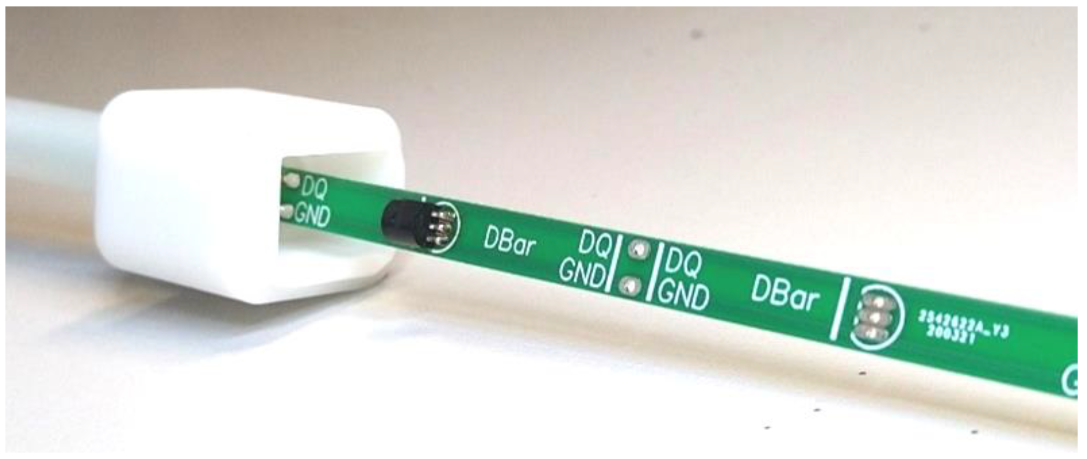
2.1. Probe Electrical Design

Our design utilizes 1-wire technology, which allows connecting multiple temperature sensors on a single twisted pair cable under certain conditions. The basis of 1-wire technology is a serial protocol using a data line and a ground reference for communication. Additional wire for device power is optional. The 1-wire master initiates and controls communication with one or more 1-wire slave devices on the 1-wire bus. Each 1-wire slave device has a unique, unchangeable, factory-programmed 64-bit identification number that serves as the device address on the 1-wire bus. The 8-bit family code, as a subset of the 64-bit ID, identifies the type and functionality of the device. Most 1-wire devices allow obtaining power for their own operation from the 1-wire bus, which is referred to as a parasitic power mode. In this case, the device does not need a third wire and just a single wire is shared for both communication and power to the device. 1-wire is widely supported by many IoT devices [30,31,32], which was another reason for our choice of sensor type DS18B20. Furthermore, in the case of a custom solution, the implementation of 1-wire protocol on a selected microcontroller is trivial. The sensors are available in packages with the dimensions of common transistors (TO-92) and IC (TSOC, TDFN, SOT23). We decided to use the variant in the TO-92 package, as it is more economically advantageous and allows easier work in laboratory conditions and the connection of sensors will use parasitic connection, as depicted in Figure 1.

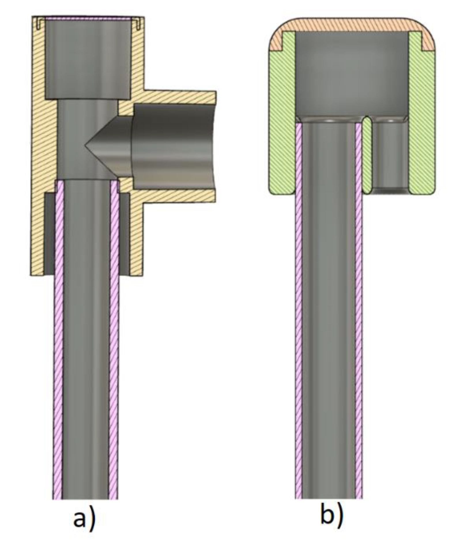
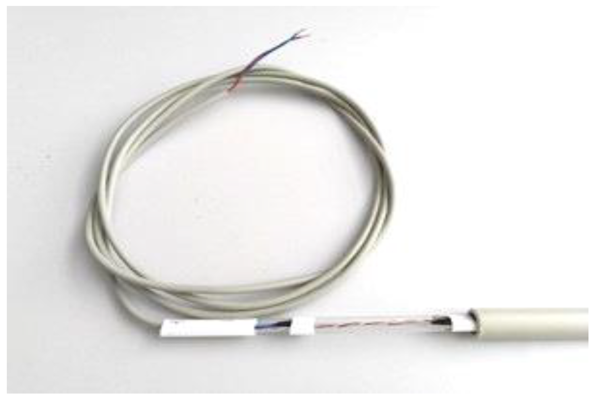
2.2. Probe Mechanical Design

For the probe mechanical parts, it is necessary to choose a material that will protect the sensory element from environmental influences, both mechanical and chemical, and others depending on the type of environment. Furthermore, concerning the parameters influencing the heat transfer through the casing, two material alternatives were chosen:
  • polypropylene as a thermoplastic polymer, which is one of the commonly used plastics in many areas of industry. It is suitable for our intended use as a probe housing due to its temperature, mechanical, and chemical resistance. A range of pipes of various diameters is available for use in plumbing installations. Various fittings are also available and the principle of joining them is with the use of a plastic welding machine,
  • polyethylene is a commonly used thermoplastic polymer. It is characterized by high resistance to acids, alkalis, and some other chemicals. It is suitable as a probe housing for measuring the temperature profile, also due to its temperature resistance. Fittings and accessories are mostly available, joining is realized by thermal fusion or by using an appropriate adhesive.
Considering the availability of materials, we decided to produce two experimental prototypes marked according to the material used as PPR for polypropylene and HDPE for polyethylene. PPR alternative—commonly available PPR components used for the implementation of plumbing installations were used to produce the probe cover. A series with a dimension of 20 mm was chosen for the housing.
Figure 2 shows a cross-section of the proposed probes interconnection pieces. We used commonly available tubing and couplings for PPR material, and we used custom made couplings for HDPE material.

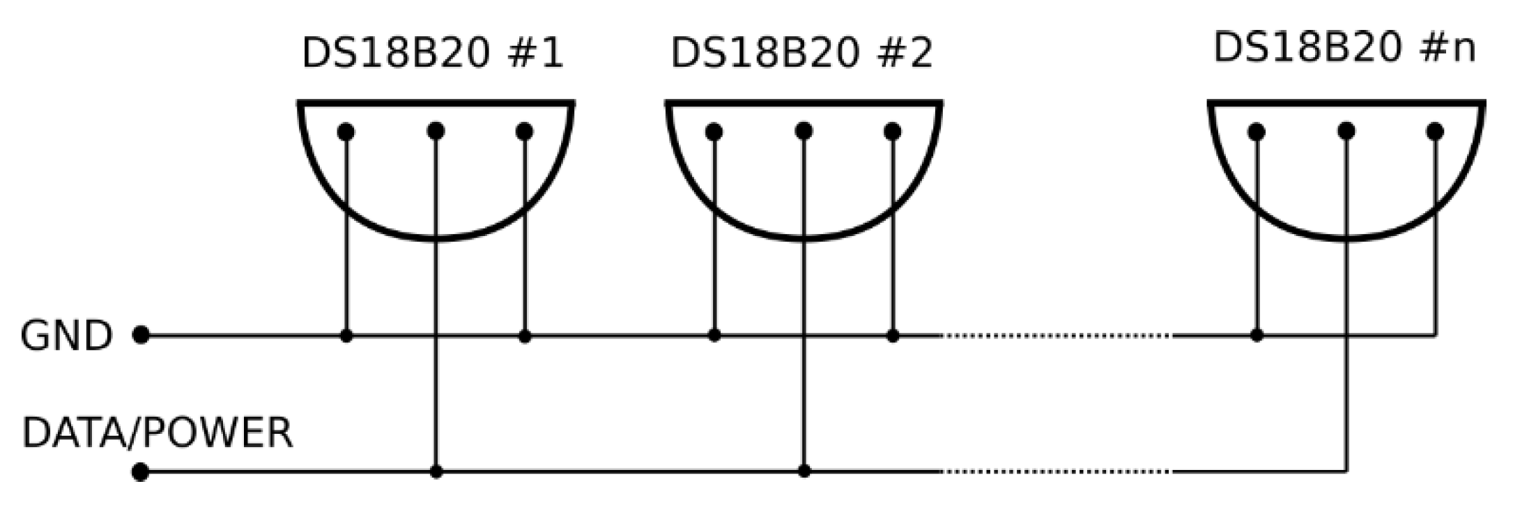
2.3. Probe Internal Connection Proposal

The basic requirement is that the sensors in the probe are placed so that they are mounted at distances precisely defined for temperature profile measurements. To achieve this goal, it is necessary to consider the need to connect the sensors to a common bus, which is physically implemented as a twisted pair cable.
Identification of individual sensors in the probe is ensured using their unique identification numbers. Connecting the sensors directly to the cable is the simplest method of implementing a temperature probe. The problem is the way to achieve the required distances between the sensors. In this case, it is necessary to add some reserve on the cable to realize bending and insulation of joints. The sensors must be attached to an auxiliary profile inserted into the housing, as shown in Figure 3.
Although this method is simple, it did not work entirely as expected. It was too laborious, and the precise placement of the sensors could not be easily ensured. Due to this fact, we proposed a method of implementing a temperature probe by connecting sensors utilizing printed circuit boards. The printed circuit boards were designed with a 50 mm grid and a module length of 250 mm in Figure 4. This modular system makes it possible to create a probe of the required length according to the immediate needs. In practice, we expect probes with lengths between 1 m and 1.5 m.
Custom dimensions of the probe can be achieved by a simple technique of cutting the PCB profile at the selected location as can be seen in Figure 5. With this method, no installation on the auxiliary profile or cable reserve is required, as the implementation only contains connecting cables to the last PCB module. The grid of 50 mm is suitable for purposes of our probe but can be modified in the future if different probe parameters are required.
When using 1-wire technology, the required cabling is reduced only to a simple twisted pair cable with copper cores. The 2 × 0.8 mm2 cable was chosen, which is commonly available in several versions for installations in both indoor and outdoor environments. An alternative is also available for placement directly in the ground or building structures (concrete, mortar, etc.). After connecting the sensors and preparing the wiring for connection to the measuring board, such a system is inserted into the prepared probe housing. Many sealing compounds are available in the market for the sealing of electronic components. For the purposes of this device, a two-component polyurethane sealant Elantron PU 310/PH 27 [33] with a recommended operating temperature of a maximum of 100 °C was chosen.

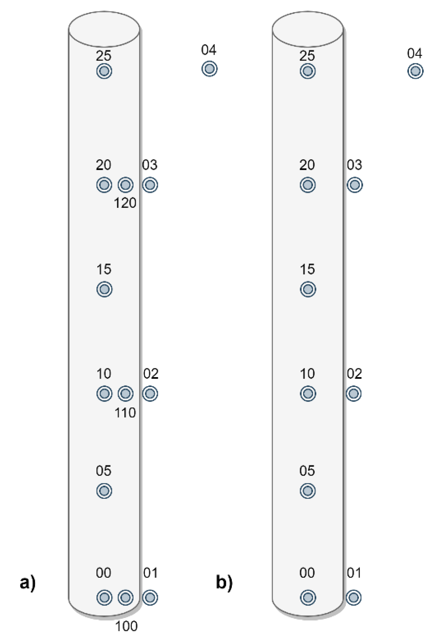
2.4. Individual Sensors Position Identification

In addition to the commonly used 64-bit sensor ID, we decided to use 2 free bytes of the non-volatile memory of the DS18B20 sensor. These are utilized to set the upper and lower limits for alarms that are used in temperature-critical applications shown in Table 1. In our design, they carry information about the position of the individual sensor in the probe, with the designation “0” for the sensor located at the bottom of the probe.
Stored value is in format: value = UBH UBL. The stored value has width of 16 bits, and the meaning of this value is position of the temperature sensor in the temperature probe.

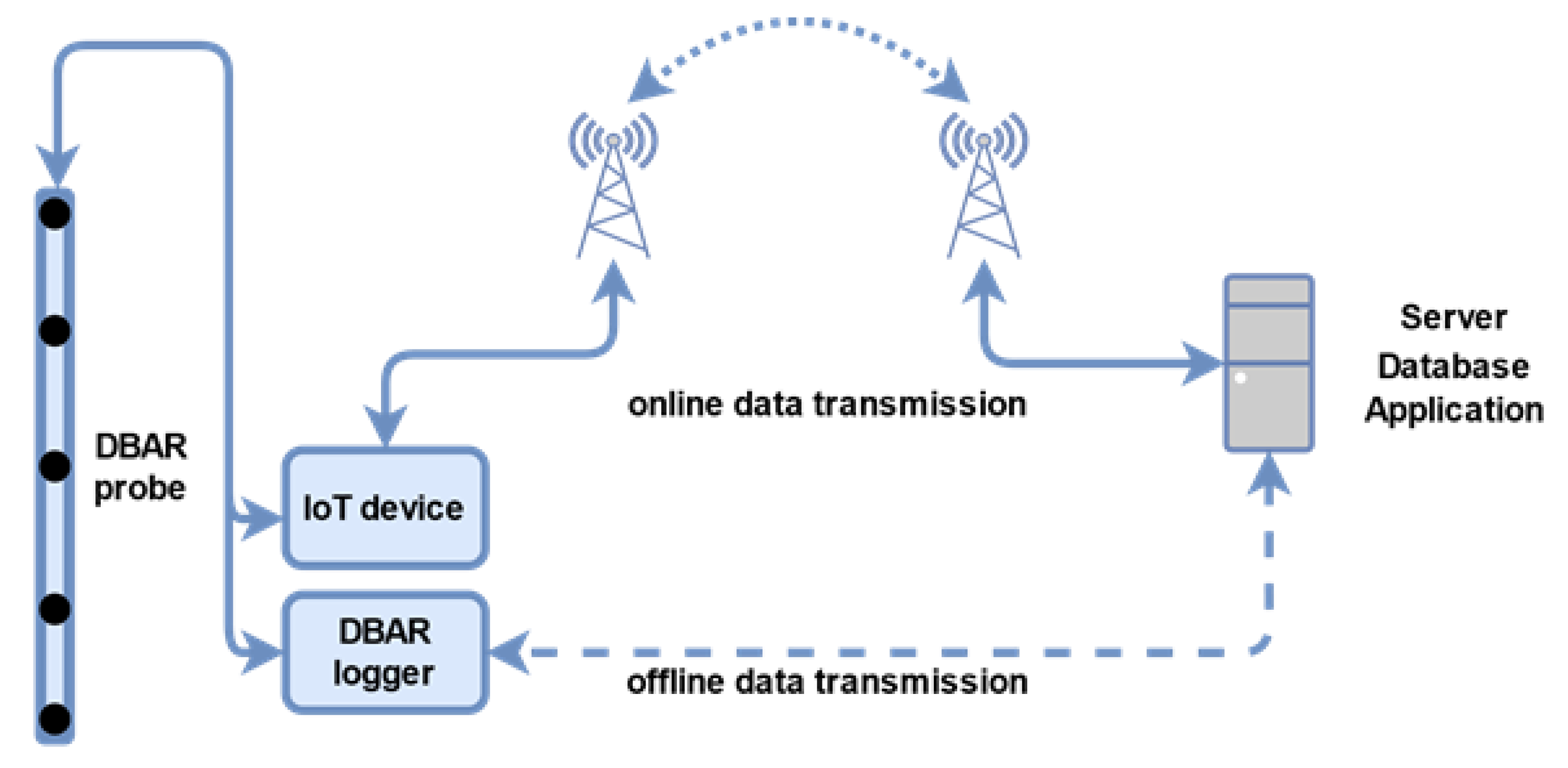
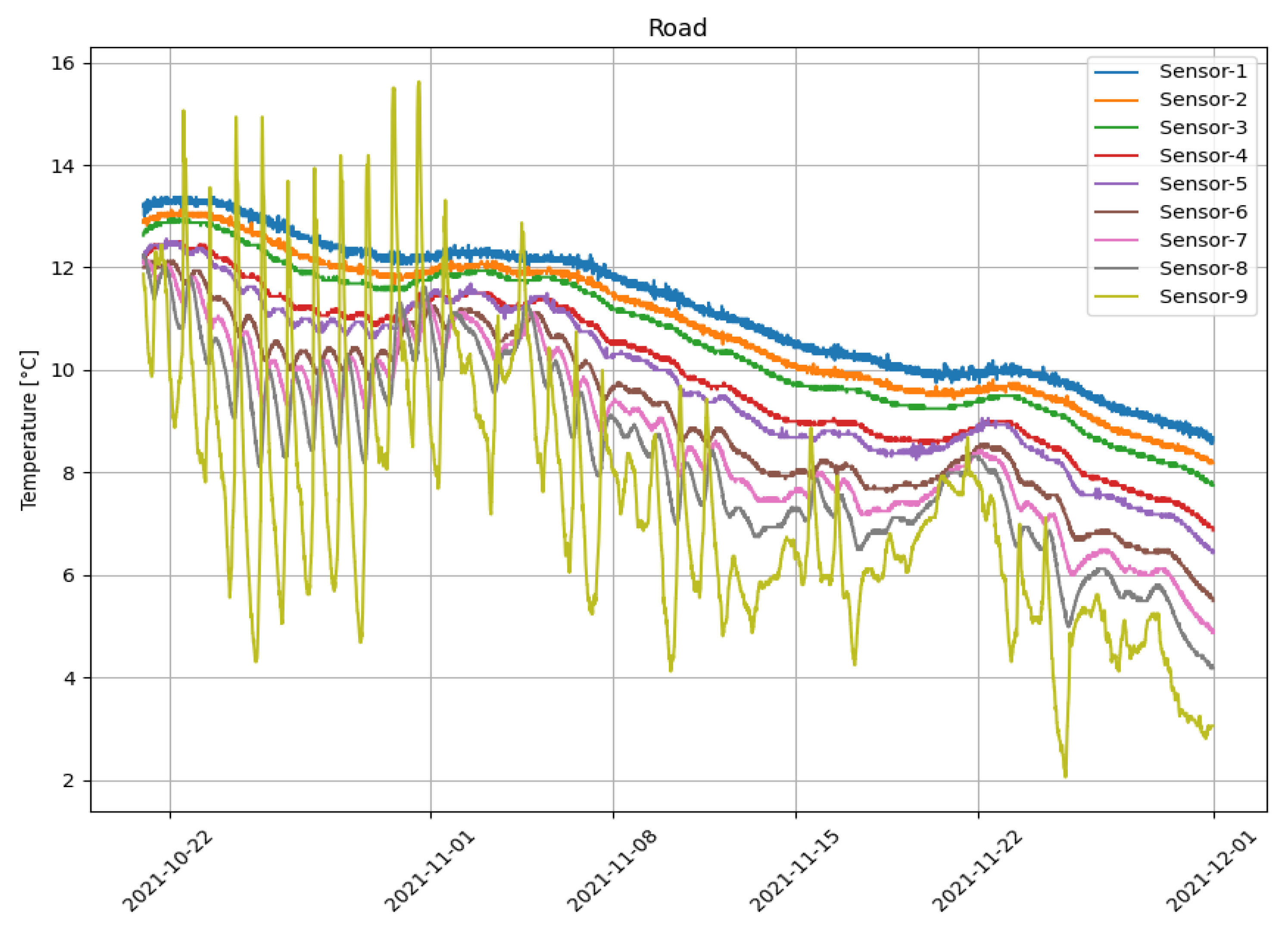
2.5. Probe System Architecture and Design for Forest Road Measurements

The probe design for measuring the vertical temperature profile of the subsoil considers the two primary applications shown in the block diagram in Figure 6. The first method is the connection of the probe to the IoT device or to the measurement control panel, which enables the online transfer of measurement data to a server solution, where the data is processed and prepared for user evaluation. The second method is collecting data into a local standalone logger, while the transfer of data to the server solution is provided by downloading data from the logger and then uploading them to the database. This solution is designed for long-term measurements, where it is not required to transmit the measured data frequently, rather it is vital to download them at specified interval as a batch.

3. Simulation Model and Experimental Measurement Proposal
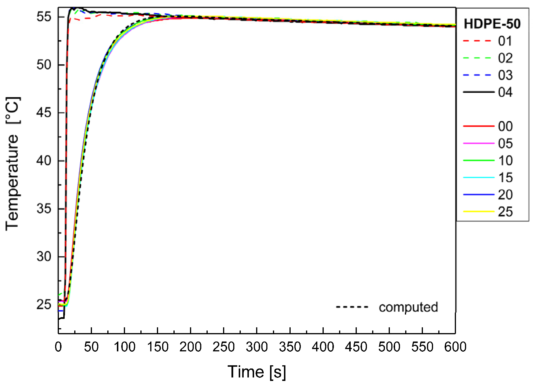
For numerical simulation of the heat transfer from the environment and experimental verification of obtained results, two experimental probes were proposed. Both probes are 250 mm long and the sensors are placed on the printed circuit boards with a 50 mm distance. The experimental probes in Figure 7 differ in the applied housing material, dimensions and the number of sensors used for proposed experiments. The decision regarding the housing material was made based on its availability on the market considering mainly its environmental resistance. Considering this, PPR and HDPE plastic materials were selected. These plastic materials offer high abrasion and corrosion resistance to soil chemicals. Both materials are also suitable in terms of operating temperature, as the experimental setup is supposed to be installed in the forest, not in a laboratory environment. Another reason is the appropriate thickness of the available plastic tubes. This property affects the heat transfer from the environment to probes attached inside the housing.
In case of probe 1 (PPR probe in Figure 7a), the probe housing is a polypropylene plastic tube with a diameter of 20 mm and a wall thickness of 3.2 mm. Sensors marked 100, 110, 120 are placed in the body of the probe with an offset of 4.5 mm from the printed circuit board, with a location corresponding to the thermometers 00, 10, 20. Sensors marked 01, 02, 03 are placed on the body of the probe with the location corresponding to the thermometers 00, 10, 20. The sensor marked 04 is, as in the case of probe 1, an auxiliary thermometer for measuring the ambient temperature.
The base construction of the probe 2 (HDPE probe in Figure 7b) uses thermoplastic polymer (HDPE material) as a tube housing material with a diameter of 10 mm and a wall thickness of 1 mm. Sensors DS18B20 marked 00, 05, 10, 15, 20, 25 are in the body of the probe with a polyurethane sealant. Sensors marked 01, 02, 03 are placed on the body surface of the probe with the location corresponding to the thermometers 00, 10, 20. The sensor marked 04 is an auxiliary sensor for measuring the ambient temperature.
There are sensors inside the tube, as we have already mentioned. These probes are encapsulated using two components consisting of a resin and curing agent. PUR sealant is used to isolate electric components from the surrounding environment to prevent damage caused by water, air humidity. Equally important, dissipation factor using PUR sealant is acceptable.
The proposed experiments covered two basic types of measurements:
(A)
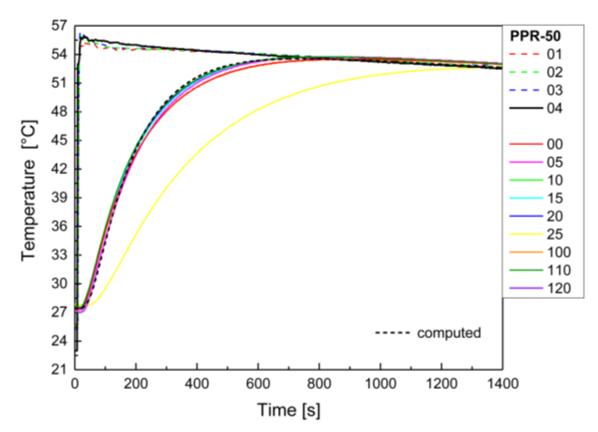
Measurement in a water bath to verify the measurement procedure during a step temperature change.
  • The measurement starts at ambient temperature.
  • The probe is immersed in a water bath at a temperature approximately 55 °C (domestic hot water).
  • The measurement is completed after approaching the temperatures measured by sensors 00, 05, 10, 15, 20, 25 and the auxiliary thermometer 04.
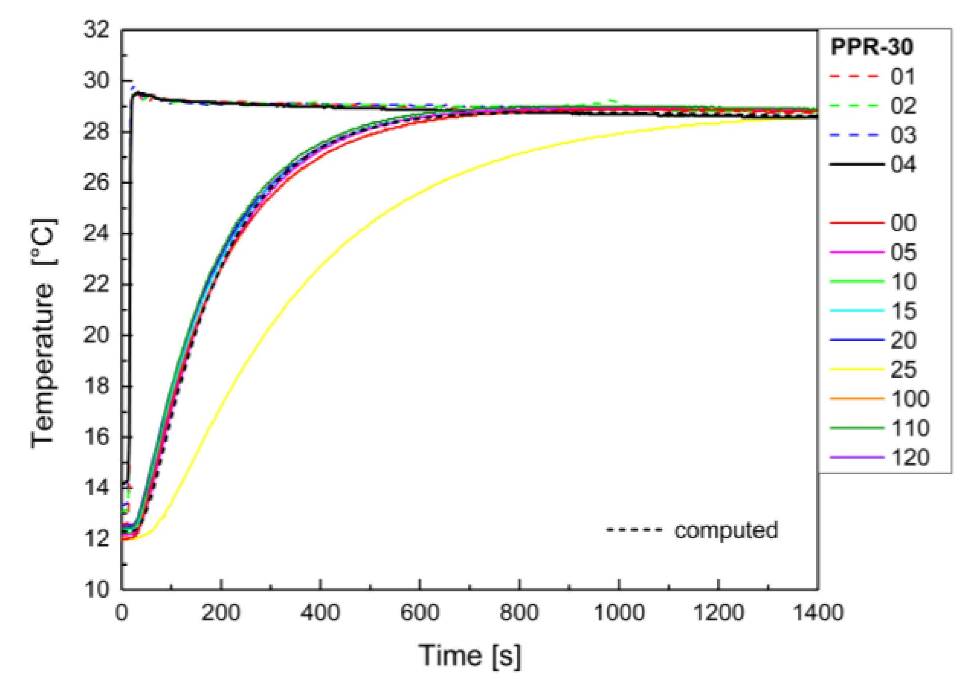
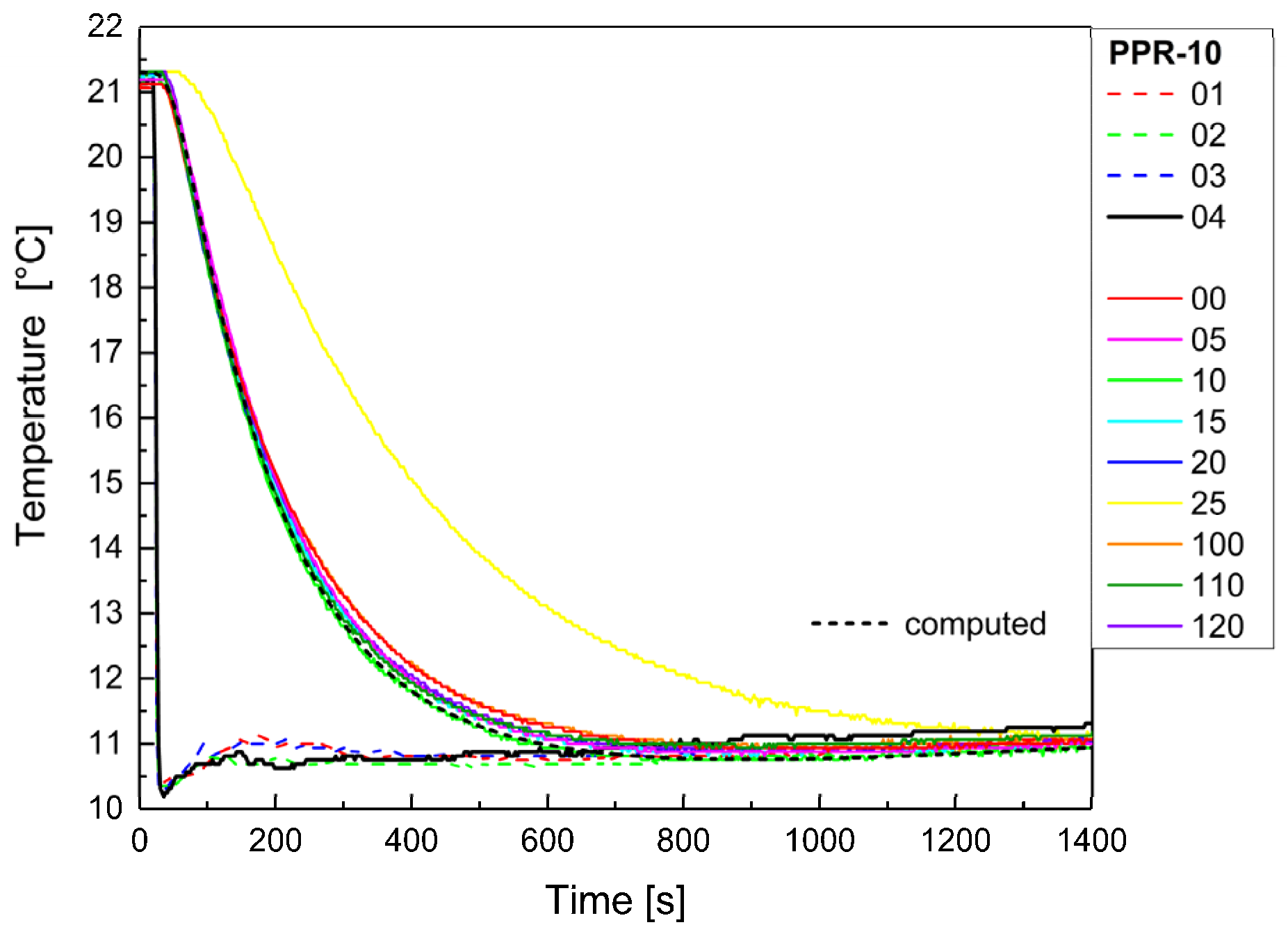
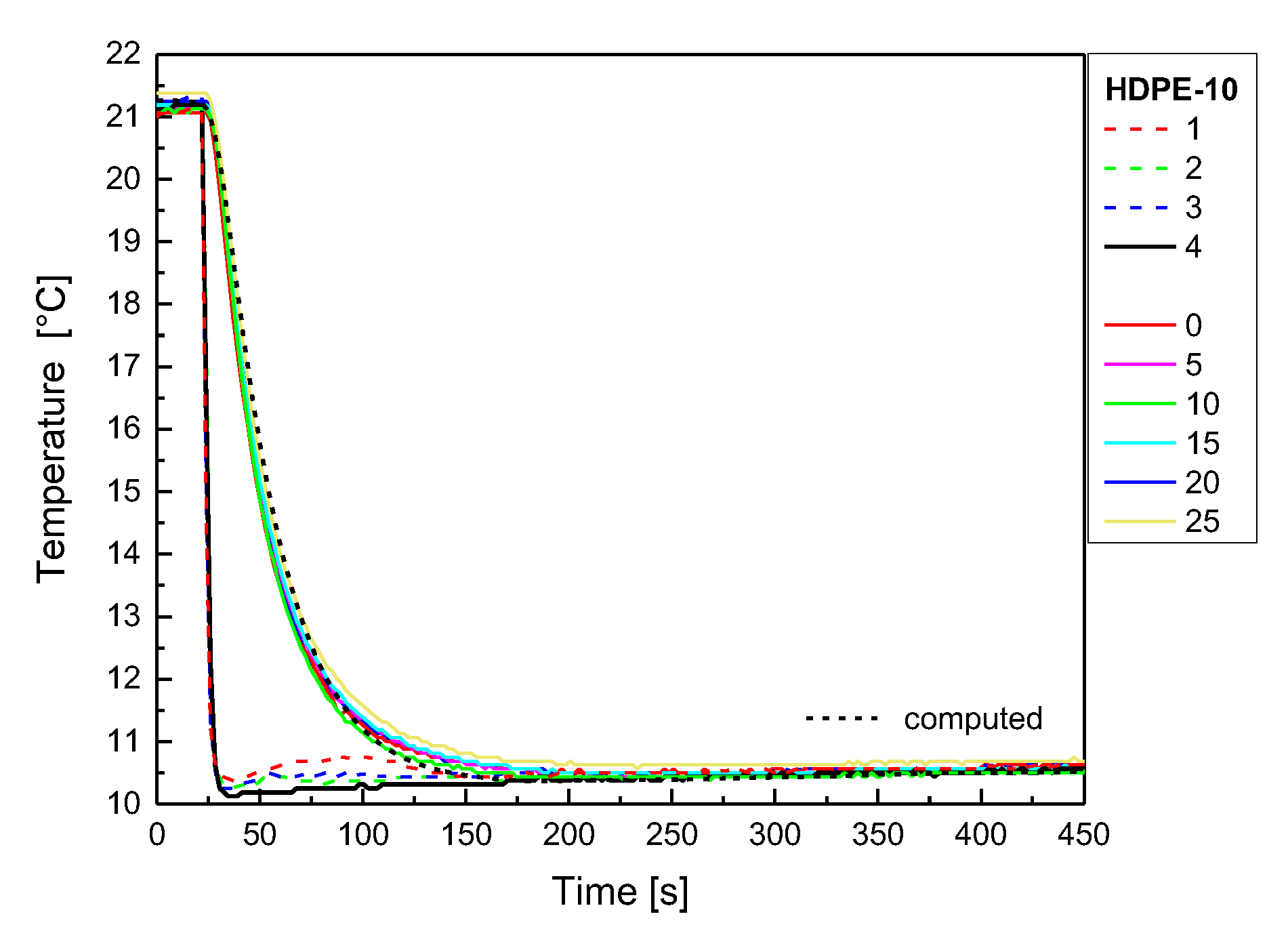
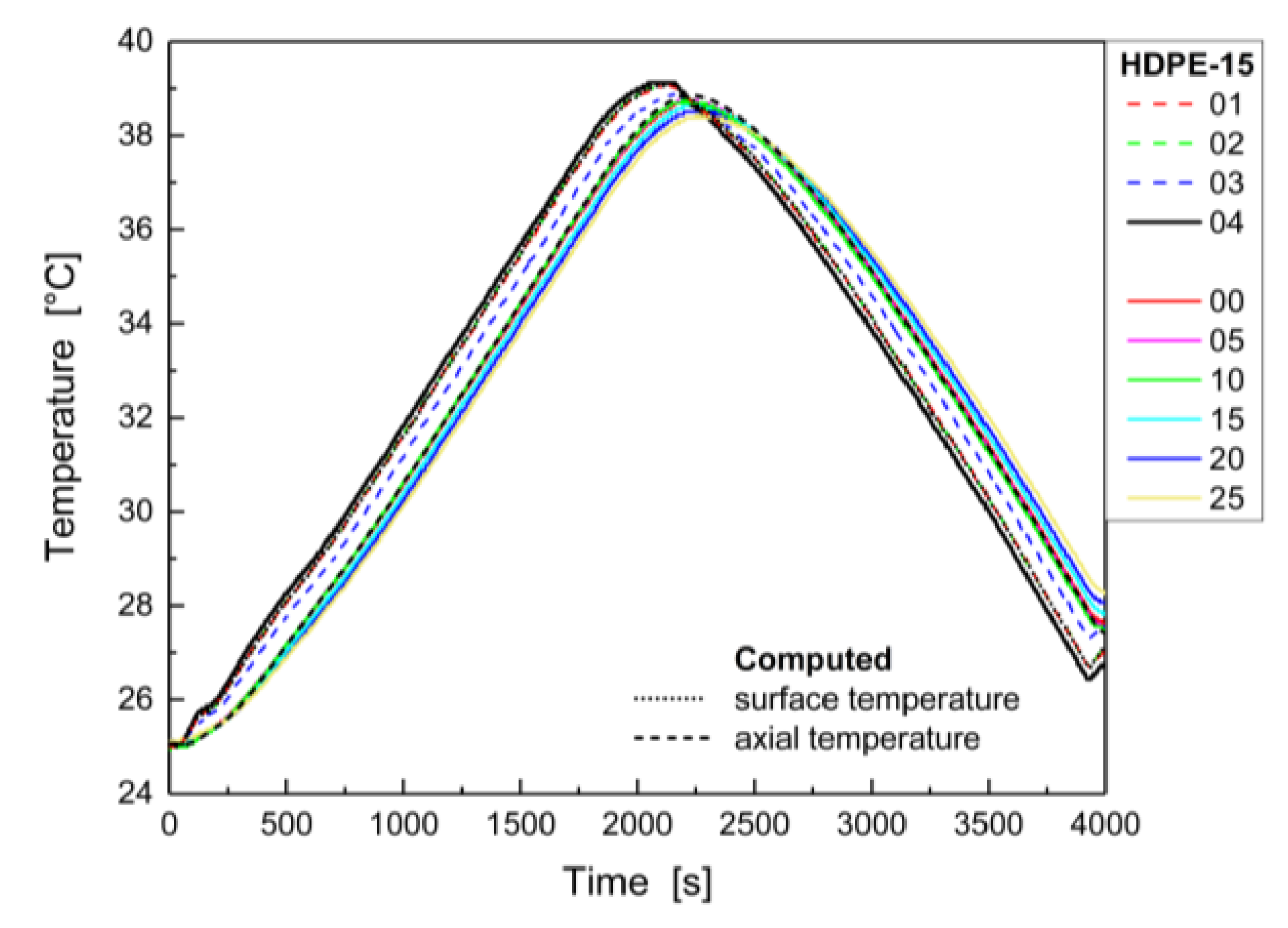
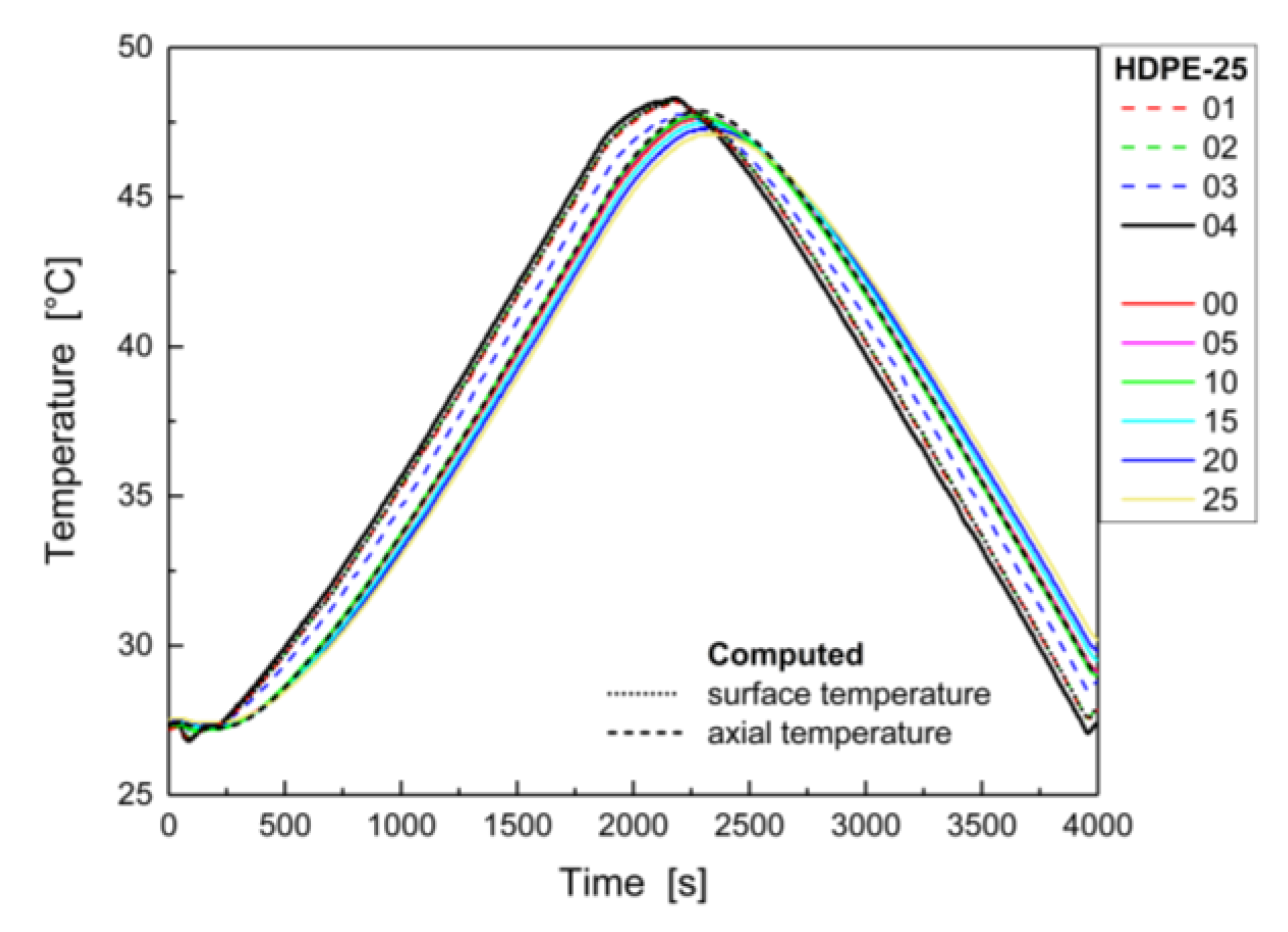
The measurement is repeated at different values of the water bath temperature (30 °C and 10 °C). The time resolution of the measurement is assumed to be ~1 s.
(B)
Measurement in a climate chamber to verify the measurement procedure in case of gradual temperature change.
  • The probe is placed into the climate chamber and the measurement starts.
  • The temperature increases by 10 °C comparing the initial temperature is adjusted in the climate chamber, followed by a dwell time of approximately 6–8 min at maximum temperature. Then the climate chamber is switched off [34].
  • The measurement is completed after approaching the temperatures measured by sensors 00, 05, 10, 15, 20, 25 and auxiliary thermometer 04.
The measurement is repeated at different maximum temperatures of the climate chamber (plus 15 °C and 25 °C). The time resolution of the measurement is assumed to be ~1 s.

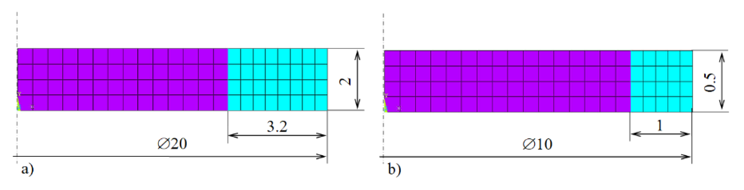
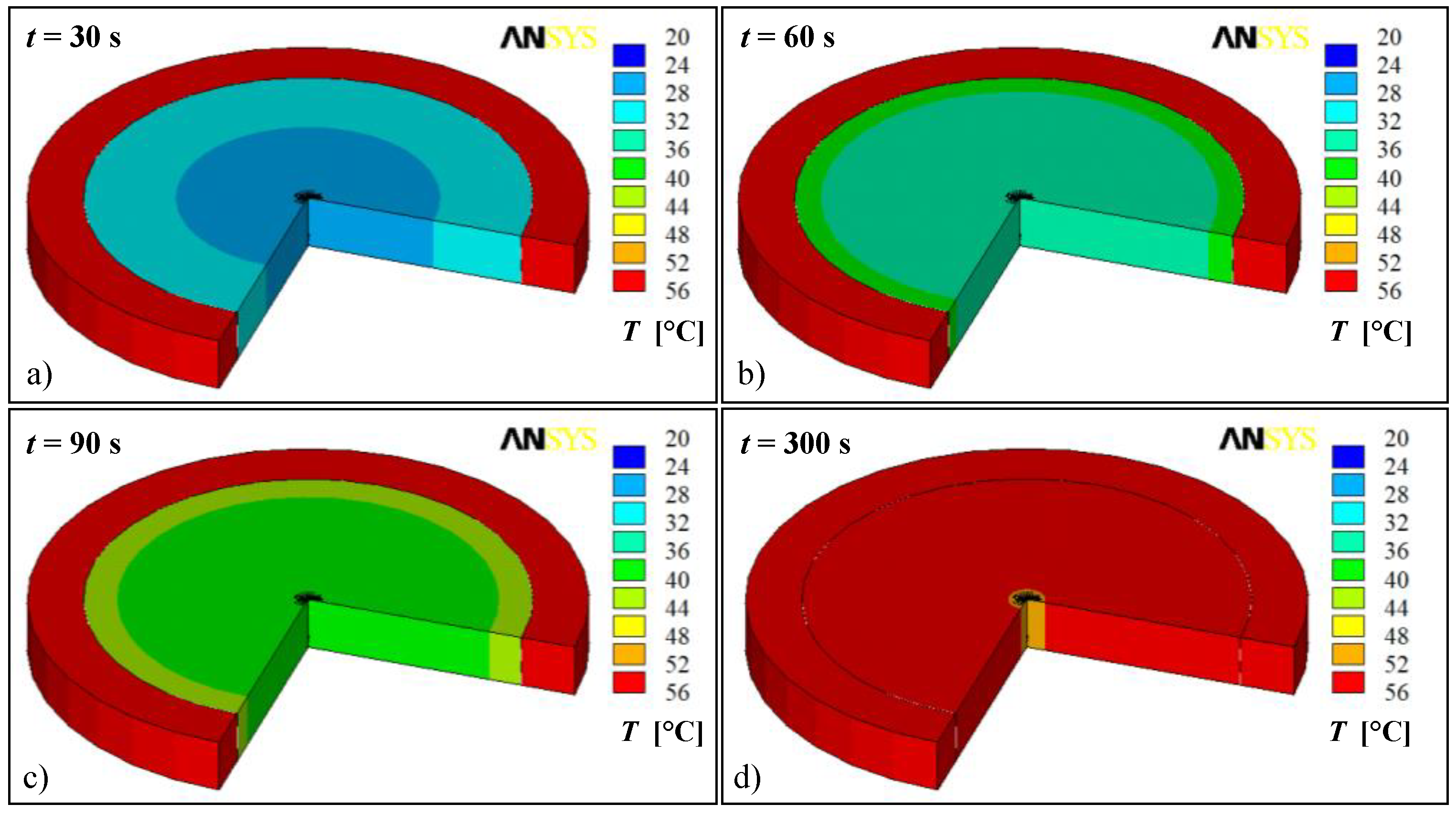
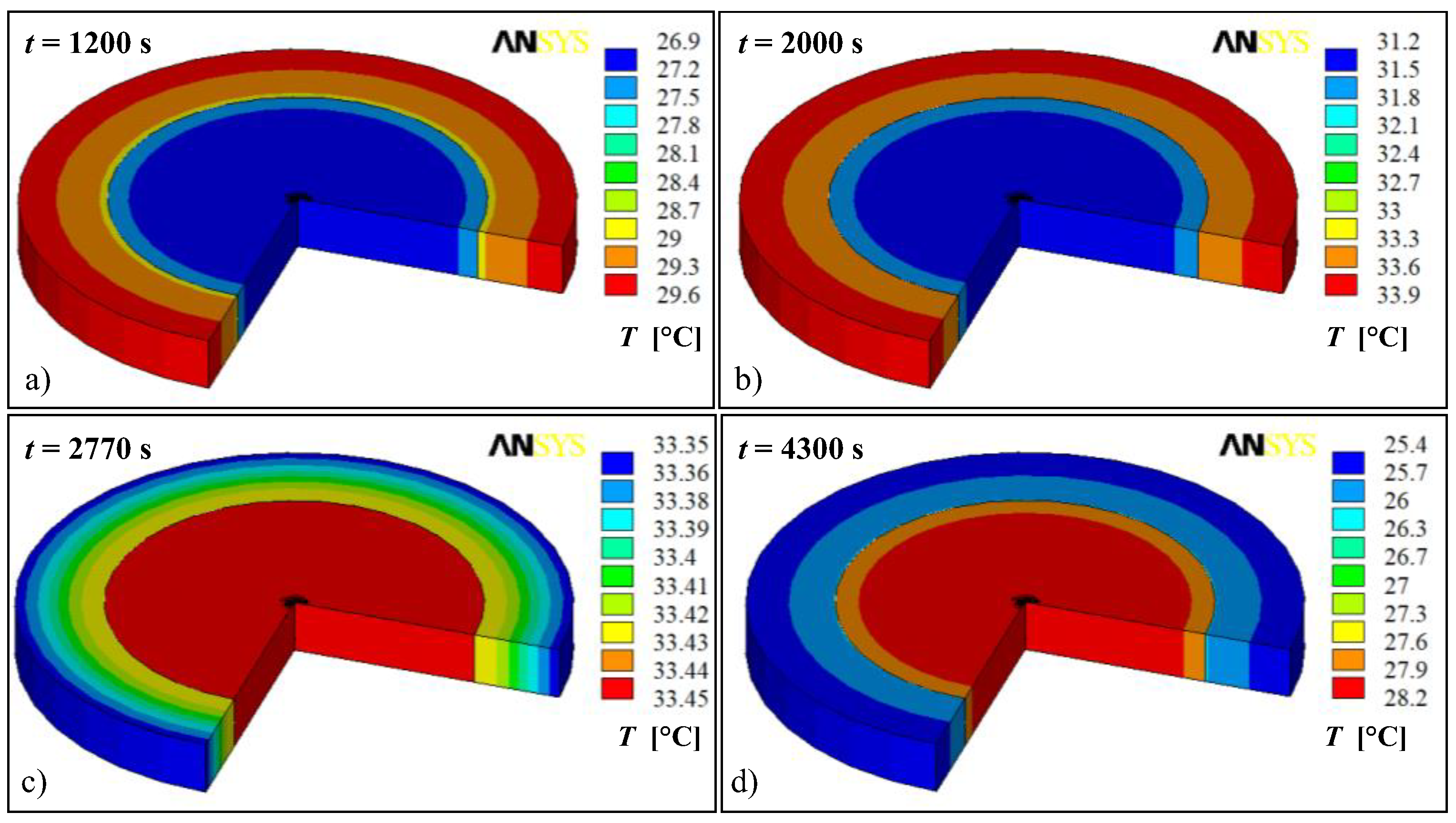
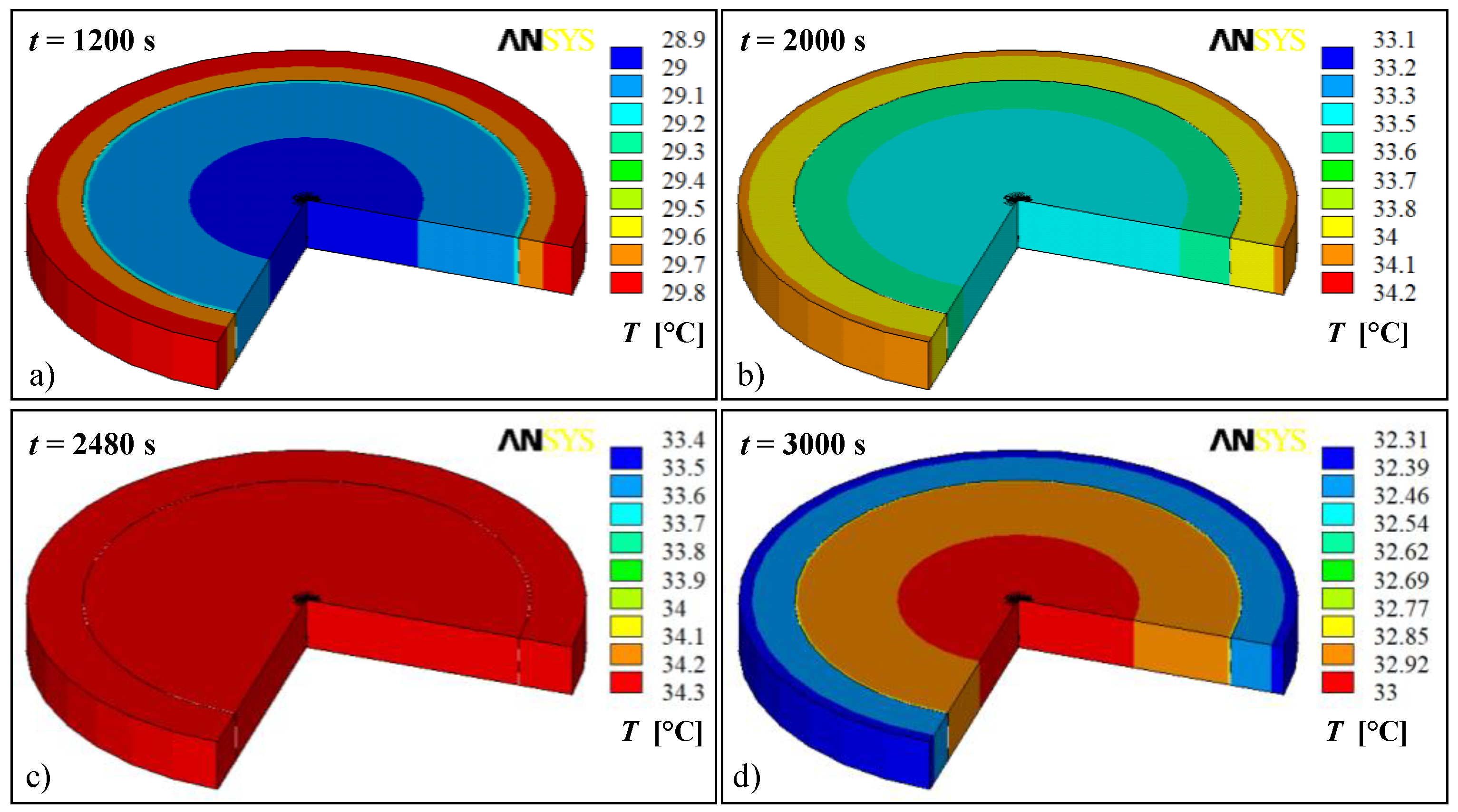
3.1. Simulation Model Proposal

Numerical simulation of temperature fields during the probe heating and cooling is based on the solution of Fourier–Kirchhoff partial differential equation in the form [35]
ρ c p T t = λ 2 T + q v ˙
in which T is the temperature, ρ is the density, cp is the specific heat, λ is the thermal conductivity, and qv is the volumetric heat source density, i.e., the heat generated per unit time in a unit volume. Geometrical, thermal, initial, and boundary conditions are necessary to define to accomplish solution of the Equation (1). Analysis of temperature fields was performed by the system ANSYS 18.1 [36] using the implemented finite element method.
Because the temperature changes along the height of the probes are negligible for the investigated heat conduction processes, it is possible to use a simplified axially symmetric model of the probe 1 and 2 with the dimensions according to Figure 8. This assumption was also confirmed by experimental measurements (see Section 4). The maximum standard deviations of the temperatures measured by the sensors in the axis of probe 1 (Figure 7a—with the exception of sensor 25) are 0.52 °C, which is at the level of accuracy of the sensors specified by the manufacturer [17]. The finite element mesh was generated using the PLANE 77 element.
The thermophysical properties of PPR and HDPE pipes as well as PUR sealant are summarized in Table 2.
The initial temperature of probes was proposed to be equal to the ambient temperature, generally 20 °C. The boundary conditions were defined in accordance with the described experimental program using the boundary condition of the 3rd type. The imperfect thermal contact between the housing wall and the PUR sealant was modeled by contact thermal resistance.

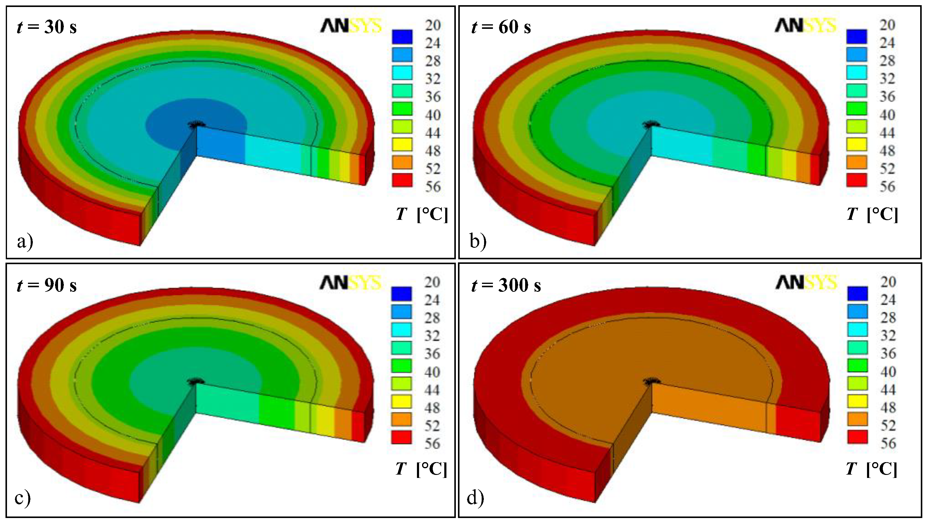
3.2. Simulation Results

Figure 9 and Figure 10 illustrate the temperature distribution in probes 1 and 2 in the time of 30 s, 60 s, 90 s, and 300 s, respectively, after immersing the probe in a water bath at approximately 55 °C. The temperature differences in the probe 2 are smaller in comparison with the probe 1. In time of 300 s, the temperatures in probe 2 are from 52 °C to 56 °C. Probe 1 has temperatures from 48 °C to 56 °C, while the temperatures of PUR sealant are from 48 °C to 52 °C. The response of the probe 1 to the sudden temperature change is delayed more.
Figure 11 and Figure 12 illustrate the temperature fields in the probe 1 and probe 2, respectively, in chosen times during probe heating and cooling in the climate chamber. Comparing the temperature distribution during the period of heating in the time of 1200 s (Figure 11a and Figure 12a) and 2000 s (Figure 11b and Figure 12b), there can be seen that the temperature rises in the probe 2 is slightly faster than in the probe 1. Minimal temperature differences of 0.1 °C in the probe 2 are reached approximately in the time of 2480 s, i.e., at the end of dwell time (Figure 12c). As it follows from Figure 11c, the minimal temperature differences in the probe 1 are during the phase of probe cooling in the time of 2770 s.

4. Simulation and Experimental Result Comparison and Discussion

To verify the simulation model, the computed and experimentally obtained results were compared. In case of measurement A (immersing the probe in a water bath), the time dependences of the temperatures measured by the sensors and the temperatures calculated in the probe axis were used in the comparison. Evaluation of time histories measured by sensors and computed on the probe surface and in the probe axis was taken into account for the measurement B (in a climate chamber).
In all the figures in this section, the time records of the temperatures measured by the sensors and thermometers marked according to Figure 7 are plotted by lines as follows: the auxiliary thermometer 04—black thick solid line; thermometers on the probe surface 01—red dashed line; 02—green dashed line; 03—blue dashed line, sensors in the probe body 00, 05, 10, 15, 20, 25; and 100, 110, 120—solid line of a specific color. The computed time histories of temperatures in the probe axis and on the probe surface are presented by black dashed lines and black dotted lines, respectively.
Figure 13, Figure 14 and Figure 15 illustrate the dependence of measured and computed temperatures on the time after immersing the probe 1 to a water bath at a temperature of 55 °C, 30 °C, and 10 °C, respectively. The temperatures measured by the sensor 25 are apparently affected by the top cover of the probe, where we used a substitute made of different material instead of a regular coupling. This problem was fixed in the experimental installation probe by using appropriate coupling cap. Otherwise, in general, a suitable match was demonstrated among the measured and calculated results. The temperature in the probe axis equalizes to the surface temperature for about 800 s after a sudden change in surrounding temperature. This time can be considered as a response time of the probe 1 to the sudden temperature change.
In Figure 16, Figure 17 and Figure 18, the time histories of measured and computed temperatures are shown for the probe 2 and measurement A. The response time in the case of probe 2 is considerably shorter. The axis temperature reaches the surface temperature approximately in the time of 250 s.
The dependences of measured and computed temperatures on the time during the measurements in a climate chamber (measurement B) are shown in Figure 19, Figure 20, Figure 21, Figure 22, Figure 23 and Figure 24. The temperature differences between the surroundings and surface temperatures, and the surface and axial temperatures for the probe 1 (Figure 19, Figure 20 and Figure 21) are larger compared to that for the probe 2 (Figure 22, Figure 23 and Figure 24). Considering the design and dimensions of probes 1 and 2, this result was expected. However, the performed measurements and calculations provide a possibility of feasible assessment of the response time of the designed probes to a gradual change of surrounding temperature. Finally, it can be concluded, that as well as in the case of measurement B, a sufficient correlation was achieved between the measured and calculated results.
For the practical verification of the probe, we carried out a pilot installation in the premises of the University of Žilina in the vicinity of other experimental installations in the field of meteorology. The probe contains nine pieces of DS18B20 thermometers spaced with 0.1 m grid. The installation was completed at the end of October 2021. The implementation is as follows: Sensor 9 is placed 0.1 m above the road surface, Sensor 8 is placed on the road surface, and Sensors 7–1 are placed 0.1 m to 0.7 m below the road surface. Figure 25 shows a graph of the temperature profile measurements from the start of the measurements in October 2021 to December 2021. Sensor 9 varies the most with respect to direct weather exposure at 0.1 m above the road surface. The effect of ambient temperature on the remaining sensors depends on their location below the road surface.
The course of measurements for one week is shown in Figure 26. It can be seen that there is a transport delay in the effect of the exterior temperature on the individual thermometers depending on their location in the probe. This phenomenon is expected and arises primarily due to the parameters of the probe installation environment, e.g., subsoil. Analyzing the results of the temperature probe 1 (Figure 19, Figure 20 and Figure 21) and probe 2 (Figure 22, Figure 23 and Figure 24) sensors, it is clear that the transport delay between the individual sensors is approximately 120 s (Probe 1) and 480 s (Probe 2). Considering the heat transfer rate in the ground (asphalt road, construction materials, subsoil) in Figure 26, where the delay among sensors is from 4 to 6 h, the own transport delay of the temperature probe is negligible.

Novelty of Proposed Solution and Future Research

The novelty of the solution can be in our opinion divided into several categories. The first category is the design of the probe itself. Commonly available solutions using, for example, thermocouples or PT sensors require extensive cabling. Typically, this involves the utilization of 2-, 3-, or 4-wire connections. Such solutions increase in physical size as the number of sensors used in the probe grows due to the need for individual cabling for each installed sensor. Cabling then represents a significant parameter affecting the probe measurements—due to the amount of wire metal used. There is a considerable degree of influence on the installed sensors and subsequent measurements. Presented solution uses a custom PCB design with glass-laminate backing and conductive copper connections. Due to the usage of DS18B20 digital thermometers, the copper used is optimized for only 2 conductive paths. Therefore, we were able to reduce the metal used significantly and thus reduce the parasite influences.
Another benefit is the possibility of deploying sensors at precisely defined distances. This is ensured by the PCB design, where in the case of our experimental probe we used a 50 mm pitch, which defines the maximum density of sensors placement. This pitch can be modified to other values such as 10 mm by simply changing the PCB design. The modularity of the probe is ensured by the usage of several PCB modules, which can be connected by jumpers and, if necessary, shortened at designated locations, which are indicated on the PCB silkscreen in front of the installed sensor.
We have designed the probe housing in two versions using two different materials. Both designs are applicable to forest road environments. The difference is perceived mainly in terms of practical installation in the forest road, taking into account the need to drill a hole with the least possible diameter in order not to disturb the subsoil and thus affect the measurements significantly. The probe uses 1-wire technology, which is widely known and often directly used in a number of available IoT solutions. This solution therefore allows the probe to be connected to data loggers, measurement control panels, stand-alone data acquisition solutions as well as online connectivity via communication converters or IoT solutions, making the probe a rather versatile device.
Furthermore, in our opinion, this is a new solution for forest roads, as the forest road area, although similar in nature to the general road area, has specific requirements for the equipment used. In our case, we have started to design a solution for the measurement of the vertical temperature profile of forest roads as part of a research project to gather information on subsoil freezing progress. In addition, the solution for the measurement of the horizontal temperature profile has already been validated from previous activities [40,41]. The said solution also uses 1-wire technology.
In additional support of our novelty claims, we note that the novelty of our solution may also be supported by the granted utility model number SK122021U1 [42].
The measured data, once processed, will enter the forest road management system, where it should be part of a predictive model for preventive maintenance and repair planning. The predictive model will have a higher relevance after the addition of other parts of the measurement system and the measurement of more annual cycles. However, this activity is not part of our temperature probe design and is beyond the scope of this manuscript.
Although the proposed probe is suitable for its intended use in the management of forest road environments, we see further opportunities for modifications and improvements in order to maximize the range of its applications. We also claimed intellectual property rights on our probe design [42]. Future research activities will aim at subtle details, which may seem to be negligible, although in overall may affect measurement characteristics of the proposed probe, for example:
  • analysis of the effect of PUR sealant aging on the response time and measurement accuracy. It is assumed that due to aging, the PUR sealant will shrink and thus the contact between the individual components of the probe will be lost. From a thermal point of view, this will increase the thermal resistance, e.g., between the probe housing and the PUR sealant, thus extending the response time;
  • investigation of temperature fields, mainly the temperature gradients along the height of the probe, which occur due to variation in the surrounding temperature depending on the time and depth in the soil layer. This research will require the preparation and solution of a 3D simulation model, including the definition of the temperature profile in the soil depending on the depth below the earth’s surface in different seasons, as well as a description of temperature changes during the day;
  • optimization of the internal probe layout with respect to self-heating of the measuring elements, space requirements and dimensions; and
  • analysis of several available sealants to design specific probe solutions for environments with special requirements.

5. Conclusions

The growing need for higher-quality transportation in a specific natural setting, typically characterized by significant temperature changes, puts pressure on local civil engineers to improve quality. The interest in more efficient forest environment management, a more pleasant approach to fire interventions, and finally, the attempt to expand recreational use of the forest in the development of tourism are the major causes for forest management. The installation of a network of stationary measuring sites on designated road sections is also part of the criteria, with the goal of providing valuable inputs for the accurate evaluation of the gathered data on the structure and road surface. This includes, for example, unique sensors that assess the temperature profile of roads in both the vertical and horizontal directions, soil sensors put along the road, frost sensors, road pollution sensors, and different meteorological sets for use on the forest road network. Our approach opens the potential of fusing data from such professional equipment with data from our suggested temperature probe for measuring the temperature profile of the soil to create a measurement set with additional value that contributes to the achievement of the above purposes.
Our proposal represents a comprehensive solution with possibilities for future extensions. We have addressed the design of the mechanical solution in two variants for use in several types of environments, considering the requirements for environments with mechanical, chemical, and environmental stresses. The electrical wiring of the sensors used is straightforward, but it was necessary to design their arrangement in the probe so that their positions were guaranteed. We proposed two solutions, of which the solution using PCB elements that can be adapted to the desired length, currently with a 50 mm grid, proved to be the most suitable. Such wiring allows data collection via a standalone logger, or the probe can be connected to an IoT device supporting a 1-wire bus. Based on the proposed solution, we have created a simulation model, which then enters the verification process. We designed and implemented a set of experiments in a water bath and a climate chamber. Subsequently, we discussed and compared the results of the experiments and simulation in Chapter 4. The presented figures clearly confirm the substantial agreement between the experimental and simulation data. Our proposed probe will primarily be used to measure the temperature profile of forest roads as input to models used in their management. However, its application is much broader in different areas of the economy, such as agriculture, energy, technological processes, automation, smart city solutions and more with requisite for measuring temperature profiles.

6. Patents

SK122021U1 Temperature probe with adjustable position of the installed sensors.

Author Contributions

Conceptualization, G.G., J.D., S.S., M.B., M.S., R.B., and B.T.; Data curation, G.G., M.B., and M.S.; Formal analysis, G.G., M.B., and M.S.; Funding acquisition, G.G. and S.S.; Investigation, J.D., S.S., R.B. and B.T.; Methodology, G.G., J.D., S.S. and M.B.; Project administration, G.G., M.S. and R.B.; Resources, G.G., J.D., S.S., M.B., and R.B.; Supervision, G.G. and M.S.; Validation, S.S., R.B., and B.T.; Writing—original draft, G.G., M.B., and R.B.; Writing—review and editing, G.G., M.B., R.B., and B.T. All authors have read and agreed to the published version of the manuscript.

Funding

This paper was supported with project of basic research: “Expanding the base of theoretical hypotheses and initiating assumptions to ensure scientific progress in methods of monitoring hydrometeors in the lower troposphere”, which is funded by the R&D Incentives contract. This paper was supported under the project of Operational Programme Integrated Infrastructure: Research and development of contactless methods for obtaining geospatial data for forest monitoring to improve forest management and enhance forest protection, ITMS code 313011V465. The project is co-funding by European Regional Development Fund.

Institutional Review Board Statement

Not applicable.

Informed Consent Statement

Not applicable.

Data Availability Statement

Not applicable.

Conflicts of Interest

The authors declare no conflict of interest.

References

  1. Roberts, R.; Inzerillo, L.; di Mino, G. Using UAV Based 3D Modelling to Provide Smart Monitoring of Road Pavement Conditions. Information 2020, 11, 568. [Google Scholar] [CrossRef]
  2. Trubia, S.; Severino, A.; Curto, S.; Arena, F.; Pau, G. Smart Roads: An Overview of What Future Mobility Will Look Like. Infrastructures 2020, 5, 107. [Google Scholar] [CrossRef]
  3. Akay, A.; Serin, H.; Sessions, J.; Bilici, E.; Pak, M. Evaluating the Effects of Improving Forest Road Standards on Economic Value of Forest Products. Croat. J. For. Eng. 2021, 42, 245–258. [Google Scholar] [CrossRef]
  4. Zhang, F.; Dong, Y.; Xu, S.; Yang, X.; Lin, H. An approach for improving firefighting ability of forest road network. Scand. J. For. Res. 2020, 35, 547–561. [Google Scholar] [CrossRef]
  5. Florková, Z.; Pepucha, L. Microtexture diagnostics of asphalt pavement surfaces. IOP Conf. Ser. Mater. Sci. Eng. 2017, 236, 12–25. [Google Scholar] [CrossRef] [Green Version]
  6. Kneib, G. Non-destructive Pavement Testing for Sustainable Road Management. In Proceedings of the 9th International Conference on Maintenance and Rehabilitation of Pavements—Mairepav9; Springer: Cham, Switzerland, 2020; pp. 675–685. [Google Scholar]
  7. Fidelus-Orzechowska, J.; Strzyżowski, D.; Cebulski, J.; Wrońska-Wałach, D. A Quantitative Analysis of Surface Changes on an Abandoned Forest Road in the Lejowa Valley (Tatra Mountains, Poland). Remote Sens. 2020, 12, 3467. [Google Scholar] [CrossRef]
  8. Kruchinin, I.N.; Pobedinsky, V.V.; Kovalev, R.N. Fuzzy simulation of forest road surface parameters. IOP Conf. Ser. Earth Environ. Sci. 2019, 316, 012026. [Google Scholar] [CrossRef]
  9. Stepanova, D.; Sukuvaara, T.; Karsisto, V. Intelligent Transport Systems–Road weather information and forecast system for vehicles. In Proceedings of the 2020 IEEE 91st Vehicular Technology Conference (VTC2020-Spring), Antwerp, Belgium, 25–28 May 2020; pp. 1–5. [Google Scholar] [CrossRef]
  10. Erhan, L.; di Mauro, M.; Anjum, A.; Bagdasar, O.; Song, W.; Liotta, A. Embedded Data Imputation for Environmental Intelligent Sensing: A Case Study. Sensors 2021, 21, 7774. [Google Scholar] [CrossRef]
  11. Wong, M.; Wang, T.; Ho, H.; Kwok, C.; Lu, K.; Abbas, S. Towards a Smart City: Development and Application of an Improved Integrated Environmental Monitoring System. Sustainability 2018, 10, 623. [Google Scholar] [CrossRef] [Green Version]
  12. Baire, M.; Melis, A.; Lodi, M.B.; Tuveri, P.; Dachena, C.; Simone, M.; Fanti, A.; Fumera, G.; Pisanu, T.; Mazzarella, G. A Wireless Sensors Network for Monitoring the Carasau Bread Manufacturing Process. Electronics 2019, 8, 1541. [Google Scholar] [CrossRef] [Green Version]
  13. Anderson, M.P. Heat as a Ground Water Tracer. Groundwater 2005, 43, 951–968. [Google Scholar] [CrossRef]
  14. García, L.; Parra, L.; Jimenez, J.M.; Parra, M.; Lloret, J.; Mauri, P.V.; Lorenz, P. Deployment Strategies of Soil Monitoring WSN for Precision Agriculture Irrigation Scheduling in Rural Areas. Sensors 2021, 21, 1693. [Google Scholar] [CrossRef]
  15. Júnior, R.D.N.; Amaral, G.C.D.; Pezzopane, J.E.M.; Toledo, J.V.; Xavier, T.M.T. Ecophysiology of C3 and C4 plants in terms of responses to extreme soil temperatures. Theor. Exp. Plant Physiol. 2018, 30, 261–274. [Google Scholar] [CrossRef]
  16. Chunpeng, H.; Yanmin, J.; Peifeng, C.; Guibo, R.; Dongpo, H. Automatic Measurement of Highway Subgrade Temperature Fields in Cold Areas. In Proceedings of the 2010 International Conference on Intelligent System Design and Engineering Application, Changsha, China, 13–14 October 2010; Volume 1, pp. 409–412. [Google Scholar] [CrossRef]
  17. Programmable Resolution 1-Wire Digital Thermometer DS18B20; Maxim Integrated Products, Inc.: San Jose, CA, USA, 2019; Available online: https://datasheets.maximintegrated.com/en/ds/DS18B20.pdf (accessed on 5 June 2021).
  18. Morais, R.; Mendes, J.; Silva, R.; Silva, N.; Sousa, J.J.; Peres, E. A Versatile, Low-Power and Low-Cost IoT Device for Field Data Gathering in Precision Agriculture Practices. Agriculture 2021, 11, 619. [Google Scholar] [CrossRef]
  19. Liu, C.; Ren, W.; Zhang, B.; Lv, C. The application of soil temperature measurement by LM35 temperature sensors. In Proceedings of the 2011 International Conference on Electronic & Mechanical Engineering and Information Technology, Harbin, China, 12–14 August 2011; Volume 4, pp. 1825–1828. [Google Scholar] [CrossRef]
  20. Izquierdo, C.G.; Garcia-Benadí, A.; Corredera, P.; Hernandez, S.; Calvo, A.G.; Fernandez, J.D.R.; Nogueres-Cervera, M.; De Torres, C.P.; Del Campo, D. Traceable sea water temperature measurements performed by optical fibers. Measurement 2018, 127, 124–133. [Google Scholar] [CrossRef] [Green Version]
  21. Othman, A.; Maga, D. Indoor Photovoltaic Energy Harvester with Rechargeable Battery for Wireless Sensor Node. In Proceedings of the 2018 18th International Conference on Mechatronics-Mechatronika (ME), Brno, Czech Republic, 5–7 December 2018; pp. 1–6. [Google Scholar]
  22. Andreadis, A.; Giambene, G.; Zambon, R. Monitoring Illegal Tree Cutting through Ultra-Low-Power Smart IoT Devices. Sensors 2021, 21, 7593. [Google Scholar] [CrossRef]
  23. Gaspar, G.; Sedivy, S.; Dudak, J.; Skovajsa, M. Meteorological support in research of forest roads conditions monitoring. In Proceedings of the 2021 2nd International Conference on Smart Electronics and Communication (ICOSEC), Trichy, India, 7–9 October 2021; pp. 1265–1269. [Google Scholar] [CrossRef]
  24. Saavedra, E.; del Campo, G.; Santamaria, A. Smart Metering for Challenging Scenarios: A Low-Cost, Self-Powered and Non-Intrusive IoT Device. Sensors 2020, 20, 7133. [Google Scholar] [CrossRef]
  25. Kampczyk, A.; Dybeł, K. The Fundamental Approach of the Digital Twin Application in Railway Turnouts with Innovative Monitoring of Weather Conditions. Sensors 2021, 21, 5757. [Google Scholar] [CrossRef]
  26. Rosero-Montalvo, P.D.; Erazo-Chamorro, V.C.; López-Batista, V.F.; Moreno-García, M.N.; Peluffo-Ordóñez, D.H. Environment Monitoring of Rose Crops Greenhouse Based on Autonomous Vehicles with a WSN and Data Analysis. Sensors 2020, 20, 5905. [Google Scholar] [CrossRef]
  27. Croce, S.; Tondini, S. Urban microclimate monitoring and modelling through an open-source distributed network of wireless low-cost sensors and numerical simulations. In Proceedings of the 7th International Electronic Conference on Sensors and Applications, Basel, Switzerland, 15–30 November 2020; p. 8270. [Google Scholar] [CrossRef]
  28. Fabo, P.; Sedivy, S.; Kuba, M.; Buchholcerova, A.; Dudak, J.; Gaspar, G. PLC based weather station for experimental measurements. In Proceedings of the 2020 19th International Conference on Mechatronics-Mechatronika (ME), Prague, Czech Republic, 2–4 December 2020; pp. 1–4. [Google Scholar] [CrossRef]
  29. Gaspar, G.; Sedivy, S.; Mikulova, L.; Dudak, J.; Fabo, P. Local Weather Station for Decision Making in Civil Engineering. In Informatics and Cybernetics in Intelligent Systems; Springer: Cham, Switzerland, 2021; pp. 199–206. [Google Scholar]
  30. Blázquez, C.S.; Piedelobo, L.; Fernández-Hernández, J.; Nieto, I.M.; Martín, A.F.; Lagüela, S.; González-Aguilera, D. Novel Experimental Device to Monitor the Ground Thermal Exchange in a Borehole Heat Exchanger. Energies 2020, 13, 1270. [Google Scholar] [CrossRef] [Green Version]
  31. Lewis, G.D.; Merken, P.; Vandewal, M. Enhanced Accuracy of CMOS Smart Temperature Sensors by Nonlinear Curvature Correction. Sensors 2018, 18, 4087. [Google Scholar] [CrossRef] [Green Version]
  32. Koritsoglou, K.; Christou, V.; Ntritsos, G.; Tsoumanis, G.; Tsipouras, M.G.; Giannakeas, N.; Tzallas, A.T. Improving the Accuracy of Low-Cost Sensor Measurements for Freezer Automation. Sensors 2020, 20, 6389. [Google Scholar] [CrossRef]
  33. Elan-tron PU 310/PH 27. ELANTAS Group. Available online: https://www.elantas.com (accessed on 16 August 2021).
  34. Vötsch Industrietechnik GmbH, “Climate Test Chambers.” March 2021. Available online: https://www.weiss-technik.com/fileadmin/Redakteur/Mediathek/Broschueren/WeissTechnik/Umweltsimulation/Voetsch/Voetsch-Technik-VC3-VCS3-EN.pdf (accessed on 15 May 2021).
  35. Incropera, F.P.; DeWitt, D.P. Fundamentals of Heat and Mass Transfer; Wiley: Hoboken, NJ, USA, 1996; Available online: https://books.google.sk/books?id=UAZRAAAAMAAJ (accessed on 16 August 2021).
  36. ANSYS, Inc. Ansys Mechanical | Structural FEA Analysis Software; Ansys: Canonsburg, PA, USA; Available online: https://www.ansys.com/products/structures/ansys-mechanical (accessed on 5 September 2021).
  37. “HDPE Data Sheet.pdf”. Available online: https://www.directplastics.co.uk/pub/pdf/datasheets/HDPE%20Data%20Sheet.pdf (accessed on 16 August 2021).
  38. “Raw Material/PPR”. Available online: http://ppr.almatherm.de/index.php?option=com_content&view=article&id=%208&Itemid=139 (accessed on 16 August 2021).
  39. Yazdi, A.; Zebarjad, S.; Sajjadi, S.; Esfahani, J. On the sensitivity of dimensional stability of high densitypolyethylene on heating rate. Express Polym. Lett. 2007, 1, 92–97. [Google Scholar] [CrossRef]
  40. Dudak, J.; Fabo, P.; Skovajsa, M.; Dvorský, L.; Kurota, P. Acta Logistica Moravica. Syst. Monit. Environ. Parameters Road Infrastruct. 2014, 4, 1804–8315. [Google Scholar]
  41. Dudak, J.; Gaspar, G.; Sedivy, S.; Pepucha, L.; Florkova, Z. Road structural elements temperature trends diagnostics using sensory system of own design. IOP Conf. Ser. Mater. Sci. Eng. 2017, 236, 012036. [Google Scholar] [CrossRef] [Green Version]
  42. Šedivý, Š.; Gašpar, G.; Fabo, P.; Farbák, M. Temperature Probe with Adjustable Position of the Installed Sensors. SK122021U1. Available online: https://worldwide.espacenet.com/patent/search/family/075979890/publication/SK122021U1?q=Gabriel%20Ga%C5%A1par (accessed on 26 May 2021).
Figure 1. Parasitic connection of sensors.
Applsci 12 00743 g001
Figure 2. Cross-sections of proposed probes: (a) PPR and (b) HDPE.
Applsci 12 00743 g002
Figure 3. Sensors connected on a cable.
Applsci 12 00743 g003
Figure 4. PCB modules for sensors.
Applsci 12 00743 g004
Figure 5. Sensors installed on a PCB module.
Applsci 12 00743 g005
Figure 6. System architecture block diagram.
Applsci 12 00743 g006
Figure 7. Experimental probes: (a) PPR and (b) HDPE.
Applsci 12 00743 g007
Figure 8. Axis-symmetric finite element model for the analysis of temperature fields (a) probe 1 (PPR) and (b) probe 2 (HDPE).
Applsci 12 00743 g008
Figure 9. Temperature distribution in the probe 1 in the time of (a) 30 s, (b) 60 s, (c) 90 s, and (d) 300 s after immersing the probe in a water bath at approximately 55 °C.
Applsci 12 00743 g009
Figure 10. Temperature distribution in the probe 2 in the time of (a) 30 s, (b) 60 s, (c) 90 s, and (d) 300 s after immersing the probe in a water bath at approximately 55 °C.
Applsci 12 00743 g010
Figure 11. Temperature distribution in probe 1 at chosen times during its heating by 10 °C and subsequent cooling in the climate chamber, (a) t = 1200 s, (b) t = 2000 s, (c) t = 2770 s and (d) t = 4300 s.
Applsci 12 00743 g011
Figure 12. Temperature distribution in probe 2 at chosen times during its heating by 10 °C and subsequent cooling in the climate chamber, (a) t = 1200 s, (b) t = 2000 s, (c) t = 2480 s and (d) t = 3000 s.
Applsci 12 00743 g012
Figure 13. Time-history of measured temperatures and the temperatures computed in the probe axis (measurement A—water bath temperature of 55 °C/probe 1).
Applsci 12 00743 g013
Figure 14. Time-history of measured temperatures and the temperatures computed in the probe axis (measurement A—water bath temperature of 30 °C/probe 1).
Applsci 12 00743 g014
Figure 15. Time-history of measured temperatures and the temperatures computed in the probe axis (measurement A—water bath temperature of 10 °C/probe 1).
Applsci 12 00743 g015
Figure 16. Time-history of measured temperatures and the temperatures computed in the probe axis (measurement A—water bath temperature of 55 °C/probe 2).
Applsci 12 00743 g016
Figure 17. Time-history of measured temperatures and the temperatures computed in the probe axis (measurement A—water bath temperature of 30 °C/probe 2).
Applsci 12 00743 g017
Figure 18. Time-history of measured temperatures and the temperatures computed in the probe axis (measurement A—water bath temperature of 10 °C/probe 2).
Applsci 12 00743 g018
Figure 19. Time-history of measured temperatures and computed surface and axial temperatures (measurement B—temperature increase in climate chamber by 10 °C/probe 1).
Applsci 12 00743 g019
Figure 20. Time-history of measured temperatures and computed surface and axial temperatures (measurement B—temperature increase in climate chamber by 15 °C/probe 1).
Applsci 12 00743 g020
Figure 21. Time-history of measured temperatures and computed surface and axial temperatures (measurement B—temperature increase in climate chamber by 25 °C/probe 1).
Applsci 12 00743 g021
Figure 22. Time-history of measured temperatures and computed surface and axial temperatures (measurement B—temperature increase in climate chamber by 10 °C/probe 2).
Applsci 12 00743 g022
Figure 23. Time-history of measured temperatures and computed surface and axial temperatures (measurement B—temperature increase in climate chamber by 15 °C/probe 2).
Applsci 12 00743 g023
Figure 24. Time-history of measured temperatures and computed surface and axial temperatures (measurement B—temperature increase in climate chamber by 25 °C/probe 2).
Applsci 12 00743 g024
Figure 25. Temperature measurements October–December 2021.
Applsci 12 00743 g025
Figure 26. Vertical temperature measurements during one week.
Applsci 12 00743 g026
Table 1. Memory map of DS1820 temperature sensor.
ScratchpadEEPROM
Byte 0–1Temperature registersNot Available
Byte 2TH Register or User Byte 1User Byte 1 (UBH)
Byte 3TL Register or User Byte 1User Byte 2 (UBL)
Byte 4Configuration registerConfiguration register
Byte 5–8ReservedNot Available
Table 2. Used materials properties [33,37,38,39].
PropertyPPRHDPEPU310/PH27
Thermal conductivity [W·m−1·K−1]0.240.40.375
Density [kg·m−3]8989561290
Specific heat [J·kg−1·K−1]200018401900
Publisher’s Note: MDPI stays neutral with regard to jurisdictional claims in published maps and institutional affiliations.

