Projection Pursuit Multivariate Sampling of Parameter Uncertainty

Abstract

The efficiency of sampling is a critical concern in Monte Carlo analysis, which is frequently used to assess the effect of the uncertainty of the input variables on the uncertainty of the model outputs. The projection pursuit multivariate transform is proposed as an easily applicable tool for improving the efficiency and quality of a sampling design in Monte Carlo analysis. The superiority of the projection pursuit multivariate transform, as a sampling technique, is demonstrated in two synthetic case studies, where the random variables are considered to be uncorrelated and correlated in low (bivariate) and high (five-variate) dimensional sampling spaces. Five sampling techniques including Monte Carlo simulation, classic Latin hypercube sampling, maximin Latin hypercube sampling, Latin hypercube sampling with multidimensional uniformity, and projection pursuit multivariate transform are employed in the simulation studies, considering cases where the sample sizes $\left(n\right)$ are small (i.e., $10\le n\le 100$), medium (i.e., $100<n\le 1000$), and large (i.e., 1000 < n≤ 10,000). The results of the case studies show that the projection pursuit multivariate transform appears to yield the fewest sampling errors and the best sampling space coverage (or multidimensional uniformity), and that a significant amount of computer effort could be saved by using this technique.

1. Introduction

Mathematical models are frequently used in many disciplines (i.e., natural sciences, social sciences, engineering) in order to realistically estimate the physical processes in question. To construct such models (or outputs), in most cases, one must use a number of input variables. For example, to calculate the original oil in place (OOIP) for a reservoir, five input variables including the thickness of the deposit, deposit area, net oil to gross volume, net porosity, and water saturation should be considered [1]. However, due to the physical and financial constraints related to the sampling scheme, there are generally a limited number of measurements (or observations) of the input variables available for modeling. Therefore, it is imperative that the effect of uncertainty associated with the input variables of the model output be taken into account [2].

There are many sampling techniques that are used to assess the uncertainty associated with the parameters of the models. For example, Monte Carlo simulation (MCS), which relies on a repeated random sampling and statistical analysis, is generally used for this purpose [3,4]. In MCS, the population is assumed to be independent and identically distributed, and the realizations of a sample are randomly chosen from the population with an equal probability. A pseudo-random number generator, which satisfies a series of statistical tests for randomness [5,6], is used to generate a sequence of independent numbers (or random variates) from a uniform distribution $U(0,1)$ [7]. A major drawback of MCS is that the realizations that are chosen completely at random tend to form clusters, which leaves gaps that are not investigated in the sampling space. If one takes a large sample of realizations, the accuracy of the predicted model output increases and the sampling errors become negligible. However, this is only achievable provided that the run time of MCS is reasonably short. If the MCS run is computationally expensive, then the sampling techniques with better sampling efficiency such as Latin hypercube sampling (LHS) (or stratified random sampling) [8,9] and its variants should be employed.

The original and most simple form of LHS is referred to as cassic Latin hypercube sampling (CLHS). In CLHS, the population is divided into a number of non-overlapping strata and MCS is used to generate a realization from each stratum. Because the population is stratified, the heterogeneity in each stratum becomes less, which results in realizations that are more uniform and representative. The stratification is maximized when the number of strata n is equal to the sample size $\left(n\right)$, i.e., $[0,1/n],[1/n,2/n],\dots ,\left[\right(n-1)/n,1]$ [10]. In CLHS, as mentioned earlier, the population is marginally stratified, that is, it accounts for only the univariate uniformity of the realizations and does not enforce any multivariate uniformity. To improve the space-filling properties of CLHS designs, many studies in the literature make use of mainly two performance criteria: (1) minimizing the pairwise correlation between the realizations, and (2) maximizing the minimum distance between the realizations [11,12,13,14,15,16]. Considering the correlated (or dependent) random variables, several studies [17,18,19,20] propose various methodologies to generate a sample whose correlation matrix is approximately equal to the given (or target) correlation matrix, that is, the joint distribution is reproduced.

The two important variants of LHS that can be used to generate realizations that have improved space-filling characteristics are (1) maximin Latin hypercube sampling (maximin LHS) [21] and (2) Latin hypercube sampling with multidimensional uniformity (LHSMDU) [1]. In the former approach, the aim is to generate a sample that maximizes the minimum Euclidean distance between any pair of realizations, which is achieved by generating a large number (i.e., thousands) of sampling designs and choosing the one that has a maximized distance between any pair of realizations. Due to the maximization of the distance between any pair, the realizations of the sample tend to spread out across the sampling space, resulting in a better multidimensional uniformity. The latter approach expands the univariate uniformity obtained by CLHS to the multivariate context. The algorithm first generates more realizations than are required, and the realizations that are close to each other (or redundant realizations) are sequentially eliminated in the multidimensional space. The post-processing of the realizations is then carried out to enforce the uniformity in the high-dimensional space.

Considering both maximin LHS and LHSMDU, it is important to note two things: (1) the realizations generated by both techniques are still based on CLHS, and (2) both techniques initially require a large number of sampling designs to be generated, which significantly increases the central processing unit (CPU) run time. A better approach for enforcing the sparsity in the sampling designs, however, would be to use projection pursuit [22,23] iterations. The idea of projection pursuit is that the projected data is expected to have a univariate Gaussian distribution if the original data is multivariate Gaussian. The original data is, therefore, generally first transformed to normal scores and then sphered so that the projection index only measures the deviation of the distribution of any projected data from the standard Gaussian distribution $N(0,1)$. The projection pursuit multivariate transform (PPMT) proposed by [24] makes use of this idea and applies a normal score transformation along a projection vector in an iterative fashion so that the original data will be eventually transformed to the uncorrelated and multivariate Gaussian scores. In fact, this amounts to saying that the multidimensional uniformity of the sampling design can be ensured through this technique.

We demonstrate the applicability of PPMT as an efficient sampling technique in two synthetic case studies using the low (bivariate) and high (five-variate) dimensional sampling spaces. The results of the simulation studies indicate that considering the various sample sizes, PPMT yields much fewer sampling errors and exhibits better space-filling characteristics than the other sampling techniques.

2. Sampling Techniques

2.1. Monte Carlo Simulation

MCS (or simple random sampling) is a technique through which a sample of the population is constructed using a random sequence of numbers. The deterministic parameters of the population can then be estimated from each sample [25]. The inverse transform method (or inversion sampling) is used to generate a realization through MCS [4]. Let Z be a random variable whose cumulative distribution function (CDF), which is monotonically non-decreasing, is denoted by $\left\{F\right(z),a\le z\le b\}$, and the inverse CDF (or a quantile function) of Z is defined by $F^{-1}\left(u\right)=\inf \{z\in [a,b]:F\left(z\right)\ge u\},0<u<1$. Considering that $U\sim U(0,1)$ is also a random variable that has a standard uniform distribution, then $z=F^{-1}\left(u\right)$, which can also be observed from $\mathrm{Pr}(Z\le z)=\mathrm{Pr}(F^{-1}\left(u\right)\le z)=\mathrm{Pr}(u\le F\left(z\right))=F\left(z\right)$.

For example, consider that $n=5$ is the required number of realizations and $k=2$ is the number of independent Gaussian random variables, $X_1\perp X_2\sim N(0,1)$, that is, the sampling space is two-dimensional and orthogonal. Independent random numbers from a uniform distribution $U(0,1)$ (i.e., the pairs exhibit a uniform distribution in the unit square, and similarly, the triplets also have a uniform distribution in the unit cube) are generated, that is, ${\mathbf{p}}_i={[p_{1i}{p}_{2i}\dots p_{ni}]}^T,i=1,\dots ,k=2$ and $n=5$. These numbers are then established in a matrix $\mathbf{P}$ where $\left(p_{ij}\right)\in {\mathbb{R}}^{5x2}$:

$$\mathbf{P}=\left[\begin{array}{cc}0.06& 0.09\\ 0.93& 0.51\\ 0.82& 0.66\\ 0.99& 0.40\\ 0.14& 0.76\end{array}\right]$$

Each element of the matrix $\mathbf{P}$ is mapped according to a target CDF, which yields the independent realizations in the Gaussian unit ${\mathbf{x}}_i={[x_{1i}{x}_{2i}\dots x_{ni}]}^T,i=1,\dots ,k=2$ and $n=5$. For instance, considering a probability of $p_{42}=0.40$ associated with the variable $X_2$, the corresponding realization can be obtained as $x_{42}=F^{-1}\left(0.40\right)=-0.24$, where $F^{-1}(·)$ denotes the inverse of the Gaussian CDF for the variable $X_2$. The MCS sampling design indicating the realizations given in matrix $\mathbf{P}$ and mapping these probabilities according to the given CDF are presented in Figure 1a,b, respectively.

The matrix $\mathbf{X}$, $\left(x_{ij}\right)\in {\mathbb{R}}^{5x2}$ whose elements are the realizations of $X_1$ and $X_2$ is then defined by

$$\mathbf{X}=\left[\begin{array}{cc}-1.54& -1.32\\ 1.44& 0.03\\ 0.90& 0.41\\ 2.31& -0.24\\ -1.08& 0.72\end{array}\right]$$

In the case where $X_1$ and $X_2$ are correlated according to a given target correlation matrix $\mathbf{C}$ where $\left(c_{ij}\right)\in {\mathbb{R}}^{2x2}$, the linear dependency between $X_1$ and $X_2$, can be added via Cholesky decompsition [26,27] of $\mathbf{C}$, that is,

$$\mathbf{C}=\mathbf{L}·{\mathbf{L}}^T,$$

(1)

where $\mathbf{L}$ is the lower triangular matrix and ${\mathbf{L}}^T$ (where the superscript T denotes transposition) is the upper triangular matrix. The correlated realizations of $X_1$ and $X_2$ are computed by multiplying the matrix $\mathbf{L}$ by the matrix ${\mathbf{X}}^T$:

$${\mathbf{X}}^{*}=\mathbf{L}·{\mathbf{X}}^T,$$

(2)

The resulting matrix ${\mathbf{X}}^{*}$ where $\left(x_{ij}^{*}\right)\in {\mathbb{R}}^{2x5}$ contains the realizations of $X_1$ and $X_2$ that have a correlation matrix, which is close to the target correlation matrix $\mathbf{C}$. The corresponding dependent quantiles (or probabilities) $0\le p_{ij}\le 1;i=1,\dots ,n=5\mathrm{and}j=1,\dots ,$$k=2$ can be drawn from the standard Gaussian CDF as $p_{ij}=F\left(x_{ij}^{*}\right)$.

2.2. Latin Hypercube Sampling

CLHS, which was proposed by McKay et al. [8], partitions each CDF of the sample of size $\left(n\right)$ from k variables into n contiguous intervals. An independent random number from the uniform distribution $p_i\in [0,1]$, $i=1,\dots ,n$ is then selected from each interval, resulting in n random numbers for each of the k variables. The aforementioned n random numbers are then randomly combined without replacements to generate the ordered quantiles.

For example, consider that the sampling space is two-dimensional $(k=2)$ and the required number of realizations is five $(n=5)$. The elements of the following matrix $\mathbf{P}$ consist of the random numbers $[0,1]$ selected from each interval of the CDFs of two random variables. The matrix $\mathbf{R}$ contains the random permutations.

$$\mathbf{P}=\left[\begin{array}{cc}0.53& 0.53\\ 0.51& 0.71\\ 0.26& 0.75\\ 0.88& 0.15\\ 0.67& 0.64\end{array}\right]\mathbf{R}=\left[\begin{array}{cc}4& 5\\ 2& 4\\ 3& 1\\ 5& 2\\ 1& 3\end{array}\right]$$

The ordered quantiles are then generated by

$$\mathbf{H}={\displaystyle \frac{1}{n}}(\mathbf{R}-\mathbf{P}),$$

(3)

The pairwise elements of the following matrix $\mathbf{H}$ indicate a stratigraphic sampling design, that is, one realization from each row and each column is generated from the sampling space, as shown in Figure 2a.

$$\mathbf{H}=\left[\begin{array}{cc}0.69& 0.89\\ 0.30& 0.66\\ 0.55& 0.05\\ 0.82& 0.37\\ 0.06& 0.47\end{array}\right]$$

Each element of the matrix $\mathbf{H}$ can then be mapped according to a target CDF as $x_{ij}=F^{-1}\left(h_{ij}\right);i=1,\dots ,n=5$ and $j=1,\dots ,k=2$, as shown in Figure 2b.

In the case of correlated random variables, the linear dependency can be added to the realizations using the Cholesky decomposition (Equation (1)).

As for maximin LHS, which is based on the distance-based criterion proposed by Johnson et al. [21], the realizations are generated by CLHS so that the minimum Euclidean distance between all of the realizations is maximized. Let w be the variable indicating the minimum distance between all of the realizations. The optimization problem can then be defined by

$$\begin{array}{c}\hfill \begin{array}{cc}\hfill \mathrm{maximize}& w\hfill \\ \hfill \mathrm{subject}\mathrm{to}& w\le ∥{\mathbf{h}}_i-{\mathbf{h}}_j∥,(i,j)\in \mathcal{J}\hfill \\ \hfill & {\mathbf{h}}_i\in \mathcal{F},i=1,\dots ,n,\hfill \end{array}\end{array}$$

(4)

where $\mathcal{J}=\{(i,j)\mid 1\le i<j\le n\},\mathbf{h}=({\mathbf{h}}_1^T,\dots ,{\mathbf{h}}_n^T)$ and ${\mathbf{h}}_i$ is the vector of coordinates for realization i in ${\mathbb{R}}^d$ with $d=2$. Considering a large number of iterations, the realizations tend to be separated from each other, allowing for a more uniform space coverage. The algorithm steps of the maximin LHS are given as follows:

• Set the initial value of the minimum Euclidean distance to zero, $w_{initial}=0$.
• Generate a sampling design $D_l,l=1,\dots ,L$ using CLHS.
• Calculate the minimum Euclidean distance $w_l$ from the CLHS design $D_l$ generated in step 2.
• If $w_l>w_{initial}$, with $l=1,\dots ,L$, set the new initial minimum Euclidean distance value as $w_l$, that is, $w_{initial}=w_l$.
• Return to step 2 and repeat the steps L times.
• End.

The algorithm steps given above are used to generate a maximin LHS design which takes into account a multidimensional uniformity through the maximization of the minimum Euclidean distance calculated from the predefined number of CLHS designs. In step 1, the initial value of the minimum Euclidean distance is equal to zero. In step 2, a CLHS design is generated. In step 3, the minimum Euclidean distance is calculated from that CLHS design, and step 4 checks if the minimum Euclidean distance calculated from the CLHS design is greater than the initial value of the Euclidean distance, which is zero. If so, the calculated minimum Euclidean distance is set as the new initial value. In step 5, the iteration is carried out a predefined number of times, and in step 6, the algorithm completes all of the iterations. A maximin LHS design where the minimum Euclidean distance is maximized considering 1000 iterations is shown in Figure 3a.

The LHSMDU algorithm proposed by Deutsch and Deutsch [1] combines CLHS with a realization elimination algorithm [28] in order to increase the multidimensional uniformity of the sampling matrix. Consider that $n=5$ represents the required number of realizations and $k=2$ is the number of random variables that are uncorrelated (or orthogonal to one another). A sampling design is generated by LHSMDU using the following steps for the algorithms:

• Generate $k·(m·n)$ random numbers from a uniform distribution $U(0,1)$, where m is an integer greater than one and the common value of m is 5 (readers are referred to Section 3 in [1] on how an appropriate m value is selected.).
• For each realization $i=1,\dots ,(m·n)$, calculate the Euclidean distance to other realizations and average the two smallest calculated distances.
• For the realization i, save the average distance and return step 2 until all of the average distances are calculated for all of the realizations $i=1,\dots ,(m·n)$.
• Remove the realization $(m·n)=(m·n)-1$ for which the smallest Euclidean distance is calculated in step 2.
• Return to step 2 and repeat the steps until the remaining number of realizations is equal to the number of realizations n that is selected initially, that is, $(m·n)=n$.
• For variable j, $j=1,\dots ,k$, rank the n realizations and use these rankings as random permutations (or a stratum).
• Generate random numbers $U(0,1)$ for the n number of strata.
• Sample the CDF of the variable j using the random numbers generated in step 7.
• Increment j, $(j=j+1)$ and return to step 6 until the ranking and sampling are carried out for all k variables.
• End.

In the case of correlated random variables, the linear dependency can be added to the realizations using the Cholesky decomposition (Equation (1)). A sampling design generated by LHSMDU with the m value equal to 5 is shown in Figure 3b.

2.3. Projection Pursuit Multivariate Transform

Considering a two-dimensional sampling space $({\mathbb{R}}^d$ where $d=2)$, a pattern (or a structure), such as clusters, outliers, and skewness, can be instantaneously discovered by simply observing the scatterplot. However, it is not possible to detect the aforementioned patterns when the sampling space is greater than three $({\mathbb{R}}^d\mathrm{where}d>3)$. Projection pursuit, which was first proposed by [22] and first implemented by [23], can be used to detect these structures in the datasets defined in a high-dimensional sampling space. It makes use of a projection index $I(\mathbf{u},\mathbf{v})$ that measures the degree of `interestingness’ of the data projected onto the plane spanned by the orthogonal vectors $(\mathbf{u},\mathbf{v})$. The plane that maximizes the projection index is determined by numerical optimization. The dataset is generally transformed to normal scores and sphered in advance, that is, the transformed data has a mean of zero, a variance of one, and an identity correlation matrix. The projection index then measures the discrepancy between the distribution of the projected data and the standard Gaussian distribution $N(0,1)$.

For example, if the data is multivariate Gaussian, all of the projections are expected to be Gaussian and no `interestingness’ will be found. Also, as proved by [29], most projections of the multivariate data appear to be approximately Gaussian under appropriate conditions. If one considers that $I(\mathbf{u},\mathbf{v})=0$ is the perfectly Gaussian case, any projected data that has a non-Gaussian distribution will increase the value of $I(\mathbf{u},\mathbf{v})$, which indicates the `interestingness’ (or non-Gaussianity). One can also consider many other projection indices that measure the deviation from the standard Gaussian distribution [30,31,32]. We use the Fortran program called PPMT.EXE, which was proposed by [24] and is publicly available through the link http://www.ccgalberta.com/resources/select-software/, accessed on 20 September 2022, in order to demonstrate the generation of a sampling design by the PPMT technique. Let us consider again that the sampling space is two-dimensional, that is, $k=2$ represents the number of random variables, and $n=5$ is the number of realizations. The steps of the PPMT procedure for generating the required number of realizations $(k·n)$ are summarized as follows:

• Generate $(k·n)$ random numbers from a uniform distribution $U(0,1)$ using MCS and establish these random numbers in a $(5\times 2)$ matrix $\mathbf{P}$.
• Transform the elements of matrix $\mathbf{P}$ to the standard Gaussian values, that is, $\mathbf{Y}=G^{-1}\left[\mathrm{F}\left(\mathbf{P}\right)\right]$, where $G^{-1}\left[\mathrm{F}(·)\right]$ is the normal score transform.
• Compute the variance–covariance matrix of $\mathbf{Y}$, that is, $\Sigma =(1/n)\left[\mathbf{Y}{\mathbf{Y}}^T\right]$.
• Diagonalize∑, that is, $\sum ={\mathbf{Q}}_1{\wedge }_1{\mathbf{Q}}_1^T$, where ${\mathbf{Q}}_1$ denotes an orthogonal matrix of the eigenvectors and ${\wedge }_1$ denotes the diagonal matrix of the eigenvalues.
• Sphere the elements of matrix $\mathbf{Y}$; that is, ${\mathbf{Y}}^{\prime }={\mathbf{S}}^{-1/2}\mathbf{Y}$, where ${\mathbf{S}}^{-1/2}={\mathbf{Q}}_1{\wedge }_1^{-1/2}{\mathbf{Q}}_1^T$.
• Project ${\mathbf{Y}}^{\prime }$ onto k-dimensional unit length vector $\mathsf{\theta }$, that is, $\mathbf{p}=\mathsf{\theta }{\mathbf{Y}}^{\prime }$.
• Determine $\mathsf{\theta }$ maximizing the projection index $I\left(\mathsf{\theta }\right)$ that measures the univariate non-Gaussianity.
• Transform ${\mathbf{Y}}^{\prime }$ to the standard Gaussian values $\widehat{\mathbf{Y}}$ so that the projection $\widehat{\mathbf{p}}=\mathsf{\theta }\widehat{\mathbf{Y}}$ is univariate Gaussian. The steps for Gaussian transformation along a projection vector of ${\mathbf{Y}}^{\prime }$ can be found in Barnett et al. [33].
• Return to step 7 until the projection index $I\left(\mathsf{\theta }\right)$ reaches convergence. The stopping criteria for the optimization can be found in [24].
• Establish the final PPMT scores as a matrix $\widehat{\mathbf{Y}}$ where $\left({\widehat{y}}_{ij}\right)\in {\mathbb{R}}^{5x2}$.
• Draw the probabilities from the standard Gaussian distribution and establish them in a matrix $\mathbf{D}=F^{-1}\left[G\left(\widehat{\mathbf{Y}}\right)\right]$, where $\left(d_{ij}\right)\in {\mathbb{R}}^{5x2}$, where $\mathbf{D}$ indicates a PPMT sampling design.
• End.

The steps given above generate a sampling design through the projection pursuit iterations. In step 1, the random realizations are generated using MCS. In steps 2–4, the realizations are transformed into the standard Gaussian values and its variance–covariance matrix is diagonalized. In step 5, the normalized realizations are sphered. The projection pursuit iterations are carried out in steps 6–9. In step 10, the final PPMT scores are generated, and in step 11, the probabilities $p_i\in [0,1]$, $i=1,\dots ,n$ are drawn from the standard Gaussian distribution. The Cholesky decomposition (Equation (1)) can be used to impose the linear correlations (or target correlation matrix) among the independent variables. A flowchart indicating the steps of the aforementioned algorithm is presented in Figure 4.

Considering the two-dimensional sampling space $(k=2)$ and $(n=5)$ realizations, a sampling design generated by PPMT mapping the probabilities according to the given CDF are shown in Figure 5a,b, respectively.

3. Case Studies

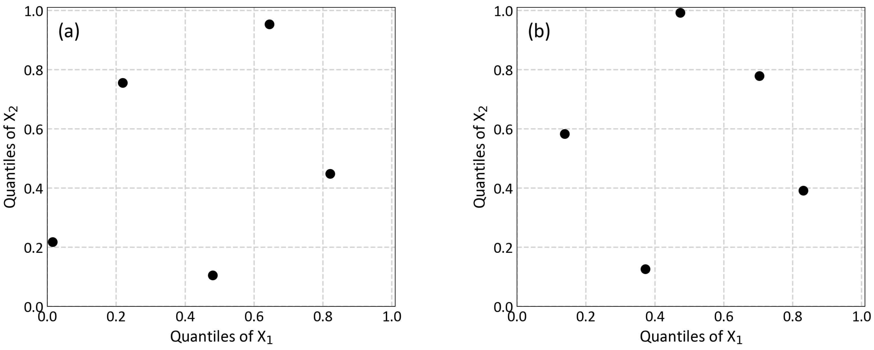
3.1. Synthetic Bivariate Case

In the first case study, we consider that the sampling space is two-dimensional $(k=2)$ and that 20 realizations $(n=20)$ of each random variable are generated using MCS, CLHS, maximin LHS, LHSMDU, and PPMT, considering the cases where the random variables are uncorrelated and correlated. It is noted that the values of the realizations that are generated are only in the range of $[0,1]$, that is, $[0,1]$ bounds are interpreted as the probability. To stabilize the distance measures between all of the realizations, 500 sets of the sample of $n=20$ are generated using each sampling technique. To assess the quality of the sampling designs yielded by each technique, we use the Wraparound L2 (WL2) statistics [34] that measure the discrepancy between the number of design realizations per subvolume in comparison to the same number of uniformly distributed realizations across the sampling space.

$$WL2=-{\left({\displaystyle \frac{4}{3}}\right)}^p+{\displaystyle \frac{1}{n^2}}\sum _{i=1}^n\sum _{j=1}^n\prod _{k=1}^p\left({\displaystyle \frac{3}{2}}-\left|z_i^k-z_j^k\right|\left(1-\left|z_i^k-z_j^k\right|\right)\right),$$

(5)

where $z_i^k$ and $z_j^k$ are the elements of the vectors ${\mathbf{z}}^1,\dots ,{\mathbf{z}}^n$; $i,j=1,\dots ,n$ denotes the number of realizations, and $k=1,\dots ,p$ denotes the number of random variables.

We first consider the case where the two random variables are uncorrelated. The realizations are straightforwardly generated by MCS and CLHS. Considering maximin LHS and LHSMDU, the additional parameters required by the procedures include the number of iterations in maximin LHS and m value in LHSMDU, as explained in Section 2.2. We select the number of iterations as 1000 in the maximin LHS procedure and consider the m value to be equal to 5 in the LHSMDU procedure. As for PPMT, the entire procedure, as explained in Section 2.3, consists of generating realizations by MCS, mapping these realizations according to a standard Gaussian CDF, using these realizations to generate PPMT scores, and back-transforming the PPMT scores to the uniform distribution. Figure 6 shows four sets of sample with $n=20$ realizations generated by MCS, CLHS, maximin LHS, LHSMDU, and PPMT.

The contours shown in Figure 6 are the probability contours of the multivariate Gaussian distribution. Because the random variables are independent, their covariance matrix is an identity matrix. Therefore, the probability contours, as shown in Figure 6, represent a circle shape.

We now consider the case where the random variables are positively correlated according to the following covariance matrix $\mathbf{C}$:

$$\mathbf{C}=\left[\begin{array}{cc}1& 0.85\\ 0.85& 1\end{array}\right]$$

As can be seen from the elements of the matrix $\mathbf{C}$, the variances of both random variables are one and the strength of the linear relation between the random variables, as determined by the covariance (or correlation coefficient), is $0.85$. The target correlation is imposed to the realizations of the independent random variables through the Cholesky decomposition (Equation (1)). Figure 7 shows the four sets of samples with $n=20$ correlated realizations generated by each sampling technique.

The contours shown in Figure 7 represent the probability contours of the multivariate Gaussian distribution. Considering the target correlation matrix $\mathbf{C}$, the probability contours exhibit an elliptical shape.

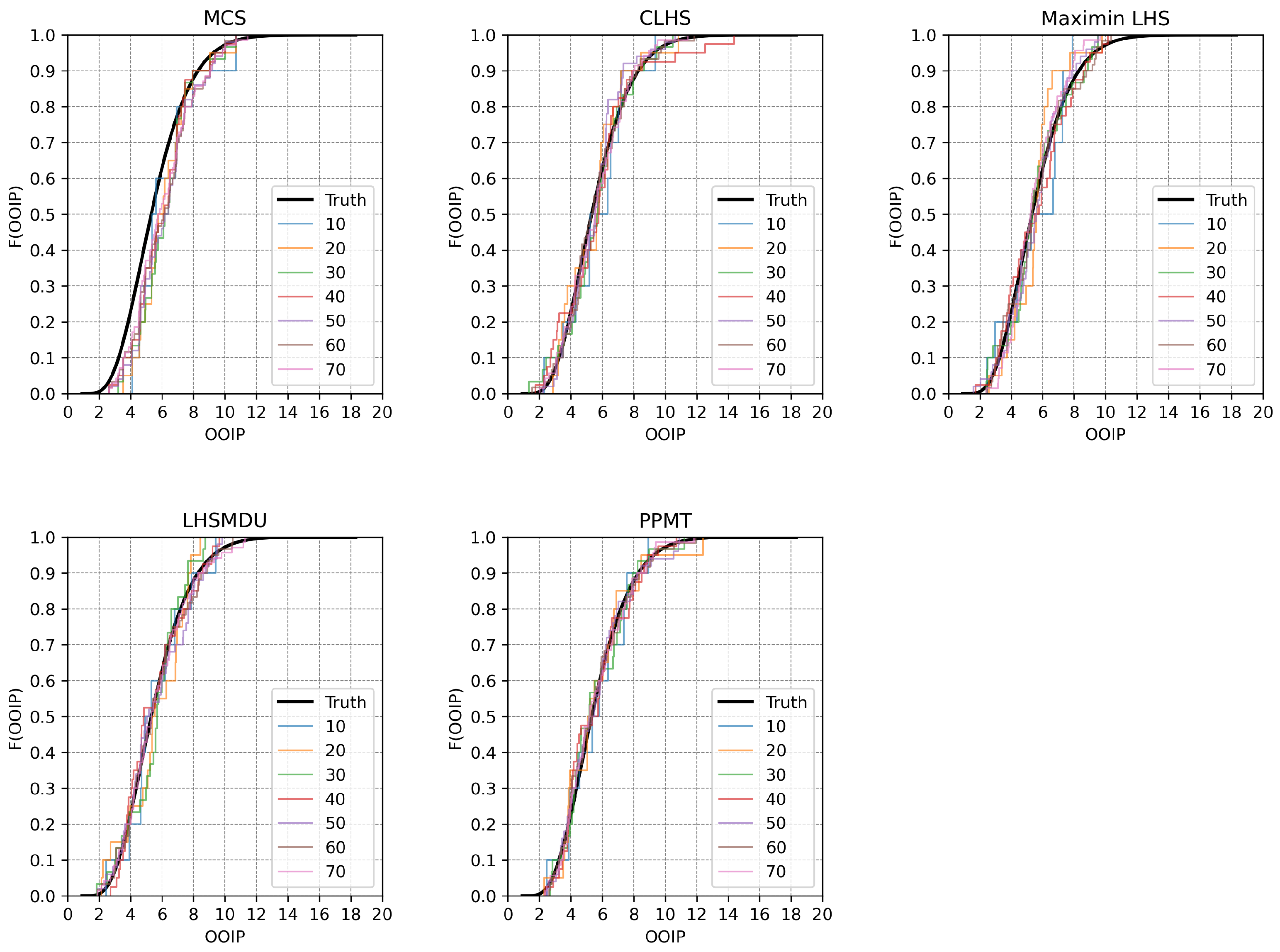
3.2. Synthetic Five-Variate Case

To further investigate the efficiency of each sampling technique, we present another case study where the sampling space is considered to be five-dimensional. We use the petroleum reservoir’s OOIP as a variable to be sampled. The formula for calculating the OOIP is given as follows:

$$\mathrm{OOIP}=\mathrm{CAT}·\mathrm{NTG}·{\varphi }_{net}(1-{\mathrm{S}}_w),$$

(6)

where $\mathrm{C}$ is the constant that accounts for units and is considered to be one; $\mathrm{A}$ represents the area of the deposit; $\mathrm{T}$ is the thickness of the deposit; $\mathrm{NTG}$ is the net oil to gross volume; ${\varphi }_{net}$ is the net porosity and ${\mathrm{S}}_w$ is the water saturation. As given in Equation (6), the value of OOIP is calculated as a function of five variables. To assess the quality of the sampling designs generated by each technique, the underlying (or truth) distribution of each OOIP variable is simulated using 10 million realizations generated by MCS. The selected distributions and their parameters for each variable are contained in

Table 1. The parametric distributions and their parameters used for each OOIP variable.

Variable	Distribution	Parameters
$\mathrm{A}$	Triangular	$a=2$, $b=4$, $c=6$
$\mathrm{T}$	Gaussian	$m=10$, $\sigma =1$
$\mathrm{NTG}$	Uniform	$a=0.6$, $b=0.8$
${\varphi }_{net}$	Triangular	$a=0.15$, $b=0.25$, $c=0.35$
${\mathrm{S}}_w$	Triangular	$a=0.15$, $b=0.2$, $c=0.3$

.

To make the results comparable to the ones shown in the study presented by Deutsch and Deutsch [1], we use the same distribution types and their parameters given in that paper. In the first part of this case study, we consider that all of the OOIP variables are uncorrelated. Given the nature of sampling, it is clear that if one takes a larger sample of realizations, the accuracy of the parameter estimation will increase. Therefore, we consider several scenarios where the sample sizes $\left(n\right)$ are relatively small $(10\le n\le 100)$, medium $(100<n\le 1000)$, and large (1000 < n ≤ 10,000). For each case, 100 sets of the predetermined sample size are generated using MCS, CLHS, maximin LHS, LHSMDU, and PPMT, that is, each of the OOIP variables is sampled from their underlying CDFs and the empirical OOIP CDF is then constructed for every sample size and every sampling technique. The efficiency of the sampling designs generated by each technique is assessed based on a criterion that is similar to the Kolmogorov–Smirnov D statistics [35], which is given as follows:

$$e=\max |F_{ref}^{-1}\left(p\right)-F_{emp}^{-1}\left(p\right)|,$$

(7)

where e is the error value indicating the maximum discrepancy between the empirical CDF generated by the particular sampling technique and the underlying CDF; $F_{ref}^{-1}\left(p\right);$$p=0.1,0.2,\dots ,0.9$ are the quantile values read from the underlying CDF; and $F_{emp}^{-1}\left(p\right);$$p=0.1,0.2,\dots ,0.9$ are the quantile values read from the empirical CDF. Figure 8 shows the underlying OOIP CDF and the randomly selected empirical CDFs of the OOIP generated by each sampling technique.

It can be seen in Figure 8 that only the empirical CDFs of the OOIP generated based on the small sample sizes are shown; this is because the greatest discrepancy between the sampling techniques should be observed in cases where the sample size is small. As the sample size increases, one should expect that the average e values calculated for each sampling technique tend to get close to one another, which can be observed in Figure 9.

The power law functions can be seen in Figure 9, which are in the form of the following equation:

$$e_{mean}=a·L^b,$$

(8)

(where L denotes the number of realizations) are fitted to the pairwise points of the average e values and the number of realizations. It is noted that the logarithmic scale is used for the x-axis shown in Figure 9. The coefficients (a and b) of the power law functions, which are contained in

Table 2. The coefficients of the power law functions in the case where the OOIP variables are uncorrelated.

Coefficients	MCS	CLHS	Maximin LHS	LHSMDU	PPMT
a	1.267	1.056	0.980	0.803	0.717
b	−0.488	−0.504	−0.484	−0.449	−0.477

, are calculated through the ordinary least squares regression.

It can be seen in Table 2 that the value of the coefficient b is approximately equal to $-0.5$ for all of the sampling techniques, the largest value of the coefficient a is obtained from the model fitted to the MCS case, and the smallest value of the coefficient a is computed from the model fitted to the PPMT case.

In the second part of this case study, we consider that the OOIP variables are somewhat correlated with one another through the following target correlation matrix $\mathbf{C}$:

$$\mathbf{C}=\left[\begin{array}{ccccc}1& 0& 0& 0& 0\\ 0& 1& 0.3& 0.25& -0.4\\ 0& 0.3& 1& 0.4& -0.5\\ 0& 0.25& 0.4& 1& -0.6\\ 0& -0.4& -0.5& -0.6& 1\end{array}\right]$$

It is clear from the elements of the matrix $\mathbf{C}$ that the first variable (thickness, $\mathrm{T}$) does not have any linear correlations with any of the remaining OOIP variables. The rest of the variables appear to be either positively or negatively correlated with one another. The Cholesky decomposition of the target correlation matrix $\mathbf{C}$ is carried out, and the independent realizations of the OOIP variables are correlated. Figure 10 shows the underlying OOIP CDF and the randomly selected empirical CDFs of the OOIP generated by each sampling technique.

The quality of the sampling designs generated by each technique is again assessed according to the criterion given in Equation (7). Figure 11 shows the plot of the averages of the e values versus the number of realizations along with the fitted power law functions.

The coefficients of the fitted models for each sampling technique are given in

Table 3. The coefficients of the power law functions in the case where the OOIP variables are correlated.

Coefficients	MCS	CLHS	Maximin LHS	LHSMDU	PPMT
a	1.577	1.297	1.244	1.118	1.028
b	−0.504	−0.492	−0.513	−0.466	−0.497

.

One can see in Table 3 that the values of the coefficient b are approximately equal to $-0.5$ for all sampling techniques, and the values of the coefficient a appear to be systematically higher than those estimated for the uncorrelated case shown in Table 2.

3.3. Quality Assessments of Sampling Designs

The quality of each design generated by the sampling techniques is visually inspected and numerically assessed according to the magnitude of the values of each criterion given in Equations (5) and (7). Considering the first case study where the sampling space is two-dimensional, one can see in Figure 6 and Figure 7 that given the realizations generated by MCS, a large area of the sampling space is not investigated. This is mainly because MCS generates realizations completely at random; therefore, it is expected that a cluster of realizations is formed in the sampling space. The sampling designs generated by CLHS appear to be better than the ones generated by MCS. This is due to the fact that CLHS enforces the univariate uniformity of the realizations, that is, the realizations are drawn from each stratum, which guarantees that there is only one realization from each row and each column of the sampling space. However, no multidimensional uniformity is considered in CLHS. As for maximin LHS, LHSMDU, and PPMT through which one can take into account the multidimensional uniformity, the sampling designs shown in Figure 6 and Figure 7 clearly indicate significant improvements in terms of the space-filling properties of the realizations.

In addition to the visual inspection of the designs, we also numerically assess the quality of each sampling design using $WL2$ statistics (Equation (5)). The box plots indicating the distribution of the aforementioned statistic considering the cases where the random variables are uncorrelated and correlated are presented in Figure 12.

It can clearly be seen in Figure 12a,b that MCS yields the largest discrepancy values according to the $WL2$ statistic, and PPMT, on the other hand, appears to outperform CLHS, maximin LHS, and LHSMDU. This is mainly due to the fact that the sampling designs generated by PPMT have no restrictions due to the Latin hypercube design. The median value of the discrepancy generated by MCS is approximately twice as much as the those generated by CLHS and its variants. The medians of the discrepancy values generated by maximin LHS and LHSMDU are rather close and slightly lower than that generated by CLHS.

Considering the second case study, one can see in Figure 8 and Figure 10 that the empirical CDFs of the samples of varying sizes generated by PPMT appear to be closer to the underlying OOIP CDF than those generated by the other sampling techniques. It is again clear in the same figures that the most noticeable discrepancy between the empirical CDFs and the underlying OOIP CDF is in the MCS case. Similarly, Figure 9 and Figure 11 clearly show that the fewest errors indicating the discrepancy between each empirical OOIP CDF and the underlying OOIP CDF are generated by PPMT. Considering the case where the random variables are correlated, the magnitudes of the error values appear to be greater for all of the sampling techniques than the uncorrelated case; however, PPMT outperforms the other sampling techniques in the correlated case as well.

In addition to the aforementioned comparisons, one should also know how many realizations should be generated by MCS to ensure a specified statistical accuracy. This can be calculated using the error values generated by each sampling technique in the power law function (Equation (8)) that is fitted to the MCS error values versus the number of realizations.

Table 4. The equivalent number of realizations to be generated by MCS ensuring the specified sampling accuracy.

MCS Equivalent Number of Realizations
Reals#	CLHS		Maximin LHS		LHSMDU		PPMT
10	20	24	22	25	26	30	30	32
100	195	200	199	204	202	208	281	312
1000	1631	1657	1690	1703	1699	1715	3398	3401
10,000	15,948	16,144	17,055	17,899	17,064	17,956	21,034	21,945

contains the approximate number of realizations that should be generated by MCS to ensure the same statistical accuracy achieved by the other sampling techniques.

The approximate number of realizations that should be generated by MCS is calculated using the coefficients (Table 2 and Table 3) of the power law functions fitted to the MCS case considering the cases where the random variables are deemed to be uncorrelated and correlated. For example, considering the uncorrelated case, the estimated coefficients ($a=1.267$ and $b\approx -0.5$) of the power law function fitted to the MCS case are used along with the error value yielded by each sampling technique for each sample size. In other words, if we want to generate 10 realizations using CLHS, the corresponding error value is used in the power law function with the coefficients estimated for the MCS case and the equivalent number of realizations to be generated by MCS is calculated. The columns where the number of realizations are given in bold in Table 4 represent the case where the random variables are correlated. For example, considering 100 realizations, in order to maintain the same statistical accuracy observed in the PPMT case, one should generate 281 and 312 realizations using MCS in the uncorrelated and correlated cases, respectively.

4. Conclusions

The main objective of this paper was to introduce PPMT as an efficient and easily applicable tool for the assessment of parameter uncertainty of the models defined in the multidimensional sampling spaces. The study considered four other sampling techniques for comparison including MCS, which is a general technique for random sampling from a given distribution, CLHS, which is a stratified random sampling technique, and two variants, the (maximinlhs and LHSMDU) of the lhs technique. Two synthetic case studies where various sample sizes (ranging from $n=10$ to $n=\mathrm{10,000}$) were used considering two- and five-dimensional sampling spaces were conducted in order to assess the sampling performance of PPMT.

In the first case study, the sampling space was considered to be two-dimensional and $n=20$ realizations of two random variables were generated 500 times. The visual and numerical results shown in Figure 6, Figure 7, and Figure 12 clearly indicated that in comparison to the other sampling techniques, PPMT appeared to be the best technique that enforces the multidimensional uniformity among the realizations defined in a two-dimensional sampling space. When the two random variables were correlated according to the target correlation matrix, PPMT again outperformed the other sampling techniques by yielding the fewest discrepancy values.

As for the second case study where the sampling space was considered to be five-dimensional, the results of the simulation study presented in Figure 8, Figure 9, Figure 10 and Figure 11 clearly indicated that PPMT yielded the fewest sampling errors in comparison to all other sampling techniques in question and generated realizations whose empirical CDFs were rather close to the underlying CDF of the variable of interest (OOIP). The other important outcome of the simulation study, which is worth mentioning, is that the CPU capacity (or run time) required for the PPMT procedure was a lot less than those required for maximin LHS and LHSMDU. Therefore, PPMT can be considered an easily applicable technique that can be used for random sampling in Monte Carlo analysis. The Python code demonstrating the implementation of the PPMT as a sampling technique in the case of correlated random variables is available through https://github.com/Oktay-Erten/PPMT_parameter_uncertainty, accessed on 20 September 2022.

References

1. Deutsch, J.L.; Deutsch, C.V. Latin hypercube sampling with multidimensional uniformity. J. Stat. Plan. Inference 2012, 142, 763–772. [Google Scholar] [CrossRef]
2. Erten, O.; Deutsch, C. Bootstrap. In Encyclopedia of Mathematical Geosciences; Daya Sagar, B., Cheng, Q., McKinley, J., Agterberg, F., Eds.; Springer International Publishing: Cham, Switzerland, 2021; pp. 1–5. [Google Scholar]
3. James, F. Monte Carlo theory and practice. Rep. Prog. Phys. 1980, 43, 1145. [Google Scholar] [CrossRef]
4. Fishman, G. Monte Carlo: Concepts, Algorithms, and Applications; Springer Science & Business Media: Berlin, Germany, 2013. [Google Scholar]
5. Law, A.M.; Kelton, W.D.; Kelton, W.D. Simulation Modeling and Analysis; McGraw-Hill: New York, NY, USA, 2000; Volume 3. [Google Scholar]
6. Ortiz, J.C.; Deutsch, C.V. Testing pseudo-random number generators. In Third Annual Report of the Centre for Computational Geostatistics; University of Alberta: Edmonton, AB, Canada, 2001. [Google Scholar]
7. Khodadadian, A.; Taghizadeh, L.; Heitzinger, C. Optimal multilevel randomized quasi-Monte-Carlo method for the stochastic drift–diffusion-Poisson system. Comput. Methods Appl. Mech. Eng. 2018, 329, 480–497. [Google Scholar] [CrossRef]
8. McKay, M.D.; Beckman, R.J.; Conover, W.J. A comparison of three methods for selecting values of input variables in the analysis of output from a computer code. Technometrics 1979, 21, 239–245. [Google Scholar]
9. McKay, M.D. Latin hypercube sampling as a tool in uncertainty analysis of computer models. In Proceedings of the 24th Conference on Winter Simulation, Arlington, VA, USA, 13–16 December 1992; pp. 557–564. [Google Scholar]
10. Pebesma, E.J.; Heuvelink, G.B.M. Latin hypercube sampling of Gaussian random fields. Technometrics 1999, 41, 303–312. [Google Scholar] [CrossRef]
11. Jin, R.; Chen, W.; Sudjianto, A. An efficient algorithm for constructing optimal design of computer experiments. J. Stat. Plan. Inference 2005, 134, 268–287. [Google Scholar] [CrossRef]
12. Tang, B. Orthogonal Array-Based Latin Hypercubes. J. Am. Stat. Assoc. 1993, 88, 1392–1397. [Google Scholar] [CrossRef]
13. Tang, B. Selecting Latin hypercubes using correlation criteria. Stat. Sin. 1998, 8, 965–977. [Google Scholar]
14. Ye, K.Q.; Li, W.; Sudjianto, A. Algorithmic construction of optimal symmetric Latin hypercube designs. J. Stat. Plan. Inference 2000, 90, 145–159. [Google Scholar] [CrossRef]
15. Morris, M.D.; Mitchell, T.J. Exploratory designs for computational experiments. J. Stat. Plan. Inference 1995, 43, 381–402. [Google Scholar] [CrossRef]
16. Park, J.S. Optimal Latin-hypercube designs for computer experiments. J. Stat. Plan. Inference 1994, 39, 95–111. [Google Scholar] [CrossRef]
17. Iman, R.L.; Conover, W.J. A distribution-free approach to inducing rank correlation among input variables. Commun. Stat.-Simul. Comput. 1982, 11, 311–334. [Google Scholar] [CrossRef]
18. Olsson, A.M.J.; Sandberg, G.E. Latin hypercube sampling for stochastic finite element analysis. J. Eng. Mech. 2002, 128, 121–125. [Google Scholar] [CrossRef]
19. Owen, A.B. Controlling correlations in Latin hypercube samples. J. Am. Stat. Assoc. 1994, 89, 1517–1522. [Google Scholar] [CrossRef]
20. Stein, M. Large sample properties of simulations using Latin hypercube sampling. Technometrics 1987, 29, 143–151. [Google Scholar] [CrossRef]
21. Johnson, M.E.; Moore, L.M.; Ylvisaker, D. Minimax and maximin distance designs. J. Stat. Plan. Inference 1990, 26, 131–148. [Google Scholar] [CrossRef]
22. Kruskal, J.B. Toward a practical method which helps uncover the structure of a set of multivariate observations by finding the linear transformation which optimizes a new “index of condensation”. In Statistical Computation; Elsevier: Amsterdam, The Netherlands, 1969; pp. 427–440. [Google Scholar]
23. Friedman, J.H.; Tukey, J.W. A projection pursuit algorithm for exploratory data analysis. IEEE Trans. Comput. 1974, 100, 881–890. [Google Scholar] [CrossRef]
24. Barnett, R.M.; Manchuk, J.G.; Deutsch, C.V. Projection Pursuit Multivariate Transform. Math. Geosci. 2014, 46, 337–359. [Google Scholar] [CrossRef]
25. Halton, J.H. A retrospective and prospective survey of the Monte Carlo method. Siam Rev. 1970, 12, 1–63. [Google Scholar] [CrossRef]
26. Watkins, D.S. Fundamentals of Matrix Computations; John Wiley & Sons: Hoboken, NJ, USA, 2004; Volume 64. [Google Scholar]
27. Deutsch, C.V.; Journel, A.G. GSLIB Geostatistical Software Library and User’s Guide, 2nd ed.; Oxford University Press: New York, NY, USA, 1997; p. 369. [Google Scholar]
28. Deutsch, C.; Begg, S. The use of ranking to reduce the required number of realizations. Centre for Computational Geostatistics (CCG) Annual Report. 2001. Available online: http://www.ccgalberta.com/ccgresources/report03/2001-115_value_of_ranking.pdf (accessed on 20 September 2022).
29. Diaconis, P.; Freedman, D. Asymptotics of graphical projection pursuit. Ann. Stat. 1984, 12, 793–815. [Google Scholar] [CrossRef]
30. Cook, D.; Buja, A.; Cabrera, J.; Hurley, C. Grand tour and projection pursuit. J. Comput. Graph. Stat. 1995, 4, 155–172. [Google Scholar]
31. Hall, P. On polynomial-based projection indices for exploratory projection pursuit. Ann. Stat. 1989, 17, 589–605. [Google Scholar] [CrossRef]
32. Klinke, S. Exploratory Projection Pursuit: The Multivariate and Discrete Case. 1995. Available online: https://citeseerx.ist.psu.edu/viewdoc/download?doi=10.1.1.45.4509&rep=rep1&type=pdf (accessed on 20 September 2022).
33. Barnett, R.M.; Manchuk, J.G.; Deutsch, C.V. The Projection-Pursuit Multivariate Transform for Improved Continuous Variable Modeling. SPE J. 2016, 21, 2010–2026. [Google Scholar] [CrossRef]
34. Hickernell, F.J. Lattice Rules: How Well Do They Measure Up? In Random and Quasi-Random Point Sets; Hellekalek, P., Larcher, G., Eds.; Springer: New York, NY, USA, 1998; pp. 109–166. [Google Scholar]
35. Johnson, R.A.; Wichern, D.W. (Eds.) Applied Multivariate Statistical Analysis; Prentice-Hall, Inc.: Upper Saddle River, NJ, USA, 1988. [Google Scholar]
Figure 1. (a) A sampling design with n = 5 realizations generated by MCS in a two-dimensional sampling space where the random variables are independent, (b) Mapping the quantiles according to the standard Gaussian distribution using the inverse transform method.
Applsci 12 09668 g001
Figure 2. (a) A sampling design with n = 5 realizations generated by CLHS in a two-dimensional sampling space where the random variables are independent, (b) Mapping the quantiles according to the standard Gaussian distribution using the inverse transform method.
Applsci 12 09668 g002
Figure 3. A sampling design with n = 5 realizations generated by (a) maximin LHS and (b) LHSMDU in a two-dimensional sampling space where the random variables are independent.
Applsci 12 09668 g003
Figure 4. A flowchart indicating the steps for generating a sampling design using PPMT.
Applsci 12 09668 g004
Figure 5. (a) A sampling design with n = 5 realizations generated by PPMT in a two-dimensional sampling space where the random variables are independent, (b) Mapping the quantiles according to the standard Gaussian distribution using the inverse transform method.
Applsci 12 09668 g005
Figure 6. Four sets of samples with n = 20 realizations generated by each sampling technique in a two-dimensional sampling space where the random variables are independent.
Applsci 12 09668 g006
Figure 7. Four sets of samples with n = 20 realizations generated by each sampling technique in a two-dimensional sampling space where the random variables are positively correlated.
Applsci 12 09668 g007
Figure 8. The underlying CDF of the OOIP in the case where the OOIP variables are uncorrelated and the empirical CDFs are generated by each sampling technique considering the small sample sizes.
Applsci 12 09668 g008
Figure 9. The averages of the e values versus the number of realizations generated by each sampling technique considering that the OOIP variables are uncorrelated.
Applsci 12 09668 g009
Figure 10. The underlying CDF of the OOIP in the case where the OOIP variables are correlated and the empirical CDFs are generated by each sampling technique considering the small sample sizes.
Applsci 12 09668 g010
Figure 11. The averages of the e values versus the number of realizations generated by each sampling technique considering that the OOIP variables are correlated.
Applsci 12 09668 g011
Figure 12. The box plots of the W L 2 statistics: (a) uncorrelated case, and (b) correlated case.
Applsci 12 09668 g012