Article

A Multi-Source Consistency Domain Adaptation Neural Network MCDANN for Fault Diagnosis

1
School of Computer Science and Technology, Xi’an Jiaotong University, Xi’an 710049, China
2
Network Information Center, Xi’an Jiaotong University, Xi’an 710049, China
*
Author to whom correspondence should be addressed.
Appl. Sci. 2022, 12(19), 10113; https://doi.org/10.3390/app121910113
Submission received: 25 August 2022 / Revised: 24 September 2022 / Accepted: 4 October 2022 / Published: 8 October 2022

Abstract

:
As the complexity and cost of industrial systems continue to increase, so does the need for the safety and reliability of industrial systems. In recent years, in the field of mechanical fault diagnosis, methods based on deep learning are gradually gaining popularity. The traditional deep learning method assumes that the training set and the test set belong to the same working condition, which is contrary to the actual industrial process. In order to improve the general ability of the fault diagnosis model, researchers start to study the domain adaptation method. However, most domain adaptation methods do not impose constraints on the test set, which leads to the occurrence of the domain mismatch problem. This paper proposes a multi-source consistency domain adaptation neural network MCDANN, which uses sub-domain division alignment and multi-source prediction consistency to achieve fine-grained domain matching and improve the transfer accuracy of the model. This paper conducts domain adaptation experiments on the open-source bearing fault dataset CWRU and DIRG bearing dataset and compares them with other classical methods. Experiments show that in the case of a signal-to-noise ratio of −4, the MCDANN model achieves an average diagnostic accuracy of more than 96% on the CWRU dataset and the DIRG dataset on noisy fault signals from the target domain, and is superior in almost all fields than other adaptive models.

1. Introduction

With the increasing complexity and cost of industrial systems, people’s tolerance for equipment performance degradation and safety hazards is getting lower and lower, and the requirements for safety and reliability are gradually increasing. Early detection and identification of faults to avoid dangerous situations is crucial [1,2,3]. A fault is defined as a phenomenon in which the deviation between one or more parameters of the system and the normal state exceeds a certain threshold, resulting in the inability of the system to perform the specified function. Fault diagnosis is the process of discovering and distinguishing fault types in time according to the state of these parameters. The current fault diagnosis methods mainly carry out fault diagnosis from the three perspectives of signal, model and knowledge [4]. Signal-based methods require certain prior knowledge to transform [5], extract representative features in the time or frequency domain using advanced signal processing techniques [6,7], and often combined with machine learning methods or neural networks to achieve good results [8,9]. As mechanical systems become increasingly complex, developing the physical models required for model-based approaches is difficult and expensive [5]. At the same time, the increased availability of data collected from multiple monitoring sensors and the ability of artificial intelligence algorithms to process the data has brought great potential for the development of advanced data-driven approaches [10,11]. Therefore, data-driven knowledge-based methods have also become one of the current research hotspots.
With the development of deep neural networks, in recent years, intelligent fault diagnosis has ushered in a new stage of development. The latest achievements in the field of deep learning in the computer field are continuously applied to the field of fault diagnosis, such as convolutional neural networks (CNN) [12,13,14], Deep Belief Networks [15,16,17], Residual Networks [18], Deep Auto-encoder (DAE) [19] as well as the latest Attention Networks [20,21,22].
In practical applications, the training data and the actual running data often come from different distributions, so although deep learning methods have made impressive progress, these practical problems will hinder their application in the industry [23]. Specifically, its main contradiction is as follows: In practical industrial applications, the source domain labeled data and the target domain unlabeled data collected under different working conditions have different distributions, which means that the deep learning model learned on the source domain can not be directly used on the target domain data. It is better to obtain the labeled fault data of the machine on the target domain; At the same time, for rotating machines, the labeled fault data on the source domain can be artificially generated during testing, so that It can be obtained at a small cost; Bnd once it enters the actual industrial production conditions, that is, the target domain, to obtain the labeled fault data, not only requires a high time cost but also may pay huge economic losses even life costs. Therefore, to solve the above contradictions, the development of a domain adaptation model is an important method and is getting more and more attention.
Domain adaptation is mainly achieved through discrepancy-based strategies or conducting adversarial learning strategies [24]. Discrepancy-based methods try to enhance the domain similarity by measuring the distance between the source and target domains on the feature layer of the model and reducing this distance using statistical methods or machine learning methods so that the model learned on the source domain can be used on the target domain. For example, Zhang et al. combined the maximum variance discrepancy with the MMD for the feature matching [25]. Deng et al. developed an ordered spectrum transfer algorithm to transfer the target data to the source domain [26]. Zhu et al. [27] and Che et al. [28] realizes domain alignment on the last two feature extraction layers of their networks. Adversarial-based methods learn invariant features between domains by introducing a domain discriminator to encourage domain confusion [29]. Jiao et al. proposed a Double-level adversarial network that simultaneously achieves domain alignment and class alignment [30]. Based on the use of domain classifiers, Li et al. enhanced the generalization of the learned features by using multiple class classifiers [31]. Guo et al. learn domain-invariant features via a domain classifier and MMD distance [32]. Li et al. adversarial training and distance metric, and scale the vibration data to enhance robustness [33]. Zhao et al. get an accurate value of joint discrepancy by improving joint distribution adaptation [34]. In the work of Zhang et al. [35], a new framework WDCNN combined with adaptation batch normalization was proposed. The one-dimensional signal is used as input in the first convolutional layer, and convolution is performed with a wide kernel (64) to suppress high-frequency noise. Domain adaptation is then achieved by extracting the mean and variance of the target domain signal and passing them to AdaBN.
Although the above domain adaptation methods have achieved good results, they all match the features in the domain from a global perspective, without considering more fine-grained information. This may allow the model to match different classes of data between the source and target domains, a phenomenon known as domain mismatch. In order to solve this problem, people are also studying how to introduce fine-grained (such as label) information into domain matching. Zhu et al. [36] proposed a Deep Subdomain Adaption Network (DSAN), which divided the original domain into several subdomains according to the similarity of the samples and then aligns the corresponding subdomains in the source domain as well as the target domain. However, this method only has a good effect on some specific data sets, and even has the opposite effect on the bearing fault data set. In order to effectively improve the accuracy of sub-domain alignment, this paper proposes a method of multi-source prediction consistency to improve the prediction accuracy of pseudo-labels, so as to achieve more accurate sub-domain alignment.
The main contributions of this paper are as follows: (1) A domain adaptation network combining DANN [37] and LMMD is proposed; (2) Fine-grained alignment with LMMD method is greatly improved with Multi-source consistency and majority voting. (3) Experiments are performed on the CWRU and DIRG [38] dataset to demonstrate the effectiveness of the proposed method.
The rest of the paper is organized as follows: Section 2 describes the proposed method and the structure of the model. Section 3 presents the experiments and results. Section 4 discusses the pros and cons of several distance metrics, as well as the effectiveness of multi-source methods. Section 5 provides the conclusion and possible future research directions.

2. Proposed Model

In this paper, we propose a multi-source consistency domain adaptation neural network MCDANN. First, on a CNN network, a gradient reversal layer is used to connect a domain classifier with the feature extractor, and the transfer of the model between domains is realized through the adversarial training of the feature extractor and the domain classifier. For the domain mismatch problem in domain adaptation training, subdomain alignment and multi-source domain adaptation methods are used to perform more fine-grained matching on domains. Taking the label of the data as a sub-domain, the pseudo-label method is applied to realize the division and alignment of the unlabeled target domain and the labeled source domain. In order to improve the accuracy of pseudo-labels, classifiers trained in different source domains are used to predict the target domain. The pseudo-labels are determined from several groups of predictions by the method of majority voting, and the cross-entropy loss is used to calculate the difference between the predictions of each group as a consistency loss which will be added to the loss function. Extract features from data with the same label in different domains, and use LMMD to calculate the distance between them and add the distance to the loss. The proposed model framework is shown in Figure 1 and will be described in detail below.

2.1. Domain Adaptation Network Based on DANN and MK-MMD

The model proposed in this paper is based on the Domain Adversarial Neural Network (DANN) [37]. DANN is a pioneering work that uses an adversarial method to complete domain adaptation, which is inspired by the adversarial generative network. The DANN network is divided into three parts, one is the feature extractor, which maps the source domain and the target domain into a feature space with small distribution differences; the other is the label classifier, the source domain data features is obtained through the feature extractor and classified through label classifier, the loss is calculated for the classification result, and the parameters of the feature extractor and the label classifier are updated; the third is the domain classifier, the source domain data features and the target domain data features are obtained through the feature extractor, and are input to the domain classifier, the loss is calculated for the domain classification result, and the parameters of the feature extractor and the domain classifier are updated. The feature extractor and the domain classifier form an adversarial network. The feature extractor improves the ability to confuse the domain in the confrontation, and the domain classifier improves the ability of the domain classification in the confrontation, so this loss is called the adversarial loss. At the same time, the gradient reversal layer GRL is applied in this adversarial network, so that the feature extractor and domain classifier in the adversarial network can perform parameter updates at the same time. The training process of the DANN network is shown in Figure 2.
The loss function of the DANN network includes label classification loss and domain adversarial loss, as shown in Formula (1):
E = i = 1 , , N d i = 0 L y G y G f x i , y i λ i = 1 , , N L d G d G f x i , y i
where the function G f represents the feature extractor, which maps the input x i into a feature space. G y is the label classifier, giving label predictions on the data. G d is the domain classifier, used to predict the domain of the data. L y is the difference between the prediction of the label classifier and the real label, and d i = 0 means that only the source domain data is predicted. L d is the difference between the predicted domain and the real domain.
In addition, DANN introduces a gradient reversal layer which allows the loss function to be calculated as a whole, thereby realizing an end-to-end network structure. The Formula (2) of the gradient reversal layer and its derivative Formula (3) are as follows:
R λ ( x ) = x
d R λ d x = λ I
Equations (2) and (3) indicate that, on the gradient reversal layer, the data does not change during the forward propagation process, but the opposite gradient direction will be obtained during backward propagation. Using this feature, a gradient reversal layer is connected before the domain classifier. During backpropagation, the gradient result from the domain classification loss function will be automatically reversed at this layer, so that the domain classification loss and the classification loss can be a whole for training. At this time, the formula of the loss function is as shown in (4):
E = i = 1 , , N d i = 0 L y G y G f x i , y i + i = 1 , , N L d G d R λ G f x i , y i
Based on a CNN network consisting of three layers of convolution and pooling, one layer of global average pooling and two fully connected layers, we use a gradient reversal layer to connect a pattern classifier whose output is 2 categories, with the feature extractor to implement a basic domain adaptation network.
The basic domain adversarial adaptation network performs well in cross-domain diagnosis of pure signals. In various cross-domain tests, it can achieve nearly 100% accuracy on the target domain, but there is still room for improvement when it comes to the cross-domain performance of noisy signals. For example, on a noisy signal with a signal-to-noise ratio of −4, the classification of the source domain is close to 100%, while the accuracy rate on the target domain is only about 90% on average. Therefore, other methods need to be introduced to assist the domain adversary neural network to find a better feature space.
In order to further improve the accuracy of model transfer, it is worthwhile to use appropriate metrics to assist network training based on adversarial theory. In the field of transfer learning, Maximum Mean Discrepancy (MMD) distance is one of the most classic metrics. Map a distribution with a Gaussian kernel function to a point on the corresponding Reproducing Kernel Hilbert Space (RKHS), and the inner product between points can be used to describe the relationship between their corresponding distributions. The expression of MMD distance is as described in Equation (5):
MMD [ F , p , q ] : = sup f F E p f x s E q f x t
where f is a function belonging to the function domain F. The intuitive meaning of this formula is to map the data from two fields having different distributions with an arbitrary function from the defined function domain, and then take the maximum value of the expected difference of the two mapped values as the MMD distance.
In MMD, the chosen kernel function to map the source domain and the target domain is fixed, and the kernel function such as Gaussian kernel or linear kernel is selected manually. However, manual selection cannot determine which kernel function is suitable for solving the problem. To this end, Gretton et al. proposed the MK-MMD distance. That is to use multiple kernels to construct a kernel, the formula of MK-MMD is shown in (6):
d k 2 ( p , q ) E p φ x s E q φ x t H k 2
where H k is the RKHS obtained by a feature kernel k, which is defined by multiple kernels together, as shown in Formula (7):
K k = u = 1 m β u k u : β u 0 , u
Note that the kernel function of MK-MMD is obtained from m different weighted kernels, and the weight is β u .
On the basic network structure shown in Figure 2, let the target domain data also participate in the training of the label classifier, and then use the output of each layer in the label classifier as the feature space. Take the feature output of the source domain data and target domain data in these network layers, compute their MK-MMD distance, and incorporate it into the original loss function as part of the loss function. The way to apply the MK-MMD distance is shown in Figure 3, specifically, conv1, 2, 3 are convolutional layers, the gap is the global average pooling layer, fc1, 2 are fully connected layers, and these two feature extraction networks in the figure are actually the same one. A loss is obtained by calculating the mk-mmd distance of the features of different domain data from the gap layer, fc1 and fc2 layers, and added to the overall loss.
Compared with the original adversarial network, the adversarial network combined with the MK-MMD distance can achieve a certain accuracy improvement. However, the accuracy improvement by adding MK-MMD distance is still limited, and there are still different degrees of errors in cross-domain diagnosis. This is due to the existence of the domain mismatch problem. Therefore, other methods should be applied to deal with it.

2.2. MCDANN

Subdomain Division and Alignment

In the process of domain adaptation network training, when the adversarial loss and feature distance are small enough and the network approaches convergence, there are still many errors in fault identification in the target domain, and the classification accuracy remains at a certain level for a long time. If the ground truth and predicted labels are printed, it can be observed that the model will always misidentify one type of fault as another.
Therefore, DSAN [36] proposes to divide the original domain into several sub-domains according to the similarity of the samples, and then align the corresponding sub-domains from the source and target domains, as shown in Figure 4.
Based on the idea of sub-domain adaptation, this paper uses data labels as the basis for sub-domain division and aligns the features of the source domain data and the target domain data with the same label. Since the target domain is unlabeled in the training process of domain adaptation, we use the predicted pseudo-label of the target domain to align with the real label of the source domain. The label classifier obtained by supervised training on the source domain is used to predict pseudo-labels of the target domain’s data; afterward, these pseudo-labels were used to correspond to the real label of the data from the source domain, finally divide these two domains into sub-domains according to the labels and align every two subdomains having the same labels which come from the source domain and target domain, respectively.
After aligning the subdomains, the distance loss is changed from Equation (6) to the Local MMD distance (LMMD) shown in Equation (8):
d k 2 ( p , q ) = 1 C c = 1 c x i s D s w i s c φ x i s x j t D t w j t c φ x j t H k 2
Among them, c represents the label, and w represents the weight. In this paper, since the label is used as a subdomain, the definition of the weight is shown in (9):
w i s c = y i c x j , y j D y j c
However, this method relies on the predicted label from the classifier. The weight update of the label classifier still only relies on the source domain data, while no constraints are imposed on the target domain data. Since the target domain data does not have real labels that can be used to test the correctness of the predictions, it is difficult to correct the predicted labels of the classifier for data from the target domain.
Therefore, using the pseudo-label method cannot really solve the problem of domain mismatch. In the bearing data studied in this paper, using the LMMD distance is even less effective than using the MK-MMD distance. In order to improve the accuracy of pseudo-labels, a multi-source domain adaptation method is introduced in this paper.

2.3. Multi-Source Prediction Consistency

When using a single labeled source domain to align with the target domain, the fine-grained information that can be obtained is limited, and only the source domain label can help the subdomain alignment. Using data from multiple source domains with different distributions and allowing them to participate in domain adaptation training at the same time can obtain more label information. This richer label information can be used to correct the alignment of sub-domains, which can improve pseudo-label prediction accuracy. The difference between single-source domain adaptation and multi-source domain adaptation is shown in Figure 5.
Use two or more working conditions as the source domain and the remaining one as the target domain. Weighting the adversarial loss and distance loss between several source and target domains before optimizing them yields higher accuracy than using only a single working condition as the source domain.
In addition, using data from multiple source domains can also improve the accuracy of pseudo-labels prediction in the target domain. When matching different source domains and target domains, if the model transfer is successful, it means that when the label classifiers from different source domains are applied to predict the same data in the target domain, the obtained pseudo labels should be consistent. The difference between several pseudo-labels can also be added to training as a loss function. In this way, the accuracy of the pseudo-label can be greatly improved.
When using multiple source domains for training, the training of the model is divided into two stages. In the first stage, the model is trained on multiple source domains, respectively. We can obtain the label classification loss and adversarial loss from the domain discriminator on each source domain, and take out their feature output on the feature layer for subsequent calculations. At the same time, for training on each source domain, the obtained label classifier is used to predict the target domain data, and then the pseudo-label of the target domain is determined by majority voting.
In the second stage, train on the target domain data to obtain the adversarial loss of the domain discriminator, and combine the adversarial loss calculated by multiple source domain data to obtain the overall domain adversarial loss. After obtaining the feature output on the target domain, the LMMD distances are calculated with the output feature of other source domains separately according to the pseudo-label, which are then summed as the distance loss. The difference between the pseudo-labels predicted in the first stage is also calculated with cross-entropy and then taken into consideration as the consistency regularization loss.
The loss function of multi-source domain adaptation is shown in Equation (10):
E = i = 1 , , N L y s i + L d s i , t + L l s i , t + i , j = 1 , , N L c e G y s i , G y s j
where L y is the loss function of the label classifier, L d represents the domain loss function of the source domain and the target domain, L l represents the distance loss between the source domain and the target domain (using LMMD distance), and L c e is the cross entropy loss function. The difference between the pseudo-labels predicted by the classifiers trained on the different source domains is taken as the consistency regularization loss.
This model combining multiple domain losses and constraining pseudo-labels with consistency regularization is called Multi-Source Consistency Domain Adaptation Neural Network (MCDANN). MCDANN consists of three network components, which are a feature extractor, a domain classifier, and a label classifier. The feature extractor includes three network blocks, which have the same network structure, including a convolutional layer, a ReLU layer, a BatchNorm layer, a convolutional layer, and a ReLU layer. The label classifier and domain classifier have the same network structure, including a fully connected layer, a BatchNorm layer, a ReLU layer, a fully connected layer, and a Softmax layer. The network structure of the three network components in MCDANN is shown in Figure 6.
The pseudo-code of the proposed MCDANN training process is shown in Algorithm 1.
Algorithm 1 Training process of MCDANN.
Input: Source domain data D S 1 , , D S N , target domain data D t
Output: Parameters θ f , θ y , θ d in the model
1:
for i = 1 n do
2:
    Forward:
3:
          Calculate classification loss
4:
          Calculate adversarial loss
5:
          Calculate consistency loss
6:
          Get pseudo labels by majority voting
7:
          Calculate distance loss
8:
    Backward:
9:
          Calculate gradient
10:
    Update:
11:
          Update model parameter θ
12:
end for
13:
return θ f , θ y , θ d

3. Experiments

3.1. Dataset

The dataset used in this paper is the bearing dataset from Case Western Reserve University(CWRU) and Polytechnic University of Turin(DIRG). These two datasets are widely used in the domain of machine learning research and testing. We conduct comprehensive experiments with the CWRU dataset, and also validate our model on the DIRG dataset.
In the CWRU dataset, we choose the various motor loads as the domains. Under each motor load condition, faults ranging from 0.007 inches in diameter to 0.040 inches in diameter were seeded separately at the inner raceway, rolling element (i.e., ball) and outer raceway, and for the faults at the raceway, we only include those whose positions are at 6 o’clock. Besides, there is one more normal working condition for each motor load. In summary, there are four kinds of motor load and each of them has 10 fault modes. In terms of signal, use the signal collected from the driving end sensor whose sampling frequency is 12K. The bearing data of Case Western Reserve University used in this paper is shown in Table 1:
For convenience, as shown in Table 1, this paper marks the normal signal as the No. 0 fault mode, and marks the 9 fault modes from B007 to OR021 as the No. 1 to No. 9 fault modes in sequence, and marks the 4 working conditions of 0~3HP as the working conditions of No. 0~3.
The signals are processed using wavelet transform and converted into an image, and the data is enhanced by the method of overlapping sampling. Sampling is performed at every 128 signal points, which means the adjacent samples have 128 signal points that are identical. Each sample has 1024 signal points, and 880 images are collected for each type of fault mode. Under motor load condition 0, the wavelet transform image of 10 fault modes is shown in Figure 7.

3.2. Experiment Result

This paper first conducts a single-source domain adaptation experiment to verify the effectiveness of the composite model. This paper takes the working conditions (bearing loads) as the domains, trains on 10 kinds of fault modes data under each load condition, and then tests the trained model under another load condition.
The data from each domain is divided into a training set and a test set at a ratio of 8:2. For each iteration during training, the model is first trained with the training sets from the source and target domains, and then the test set from the source and target domains are used to test the performance of the model and observe the classification accuracy of the model on the source and target domains. The number of training iterations is 100 and repeated 10 times. The classification result is the average of the optimal classification accuracy on the target domain.
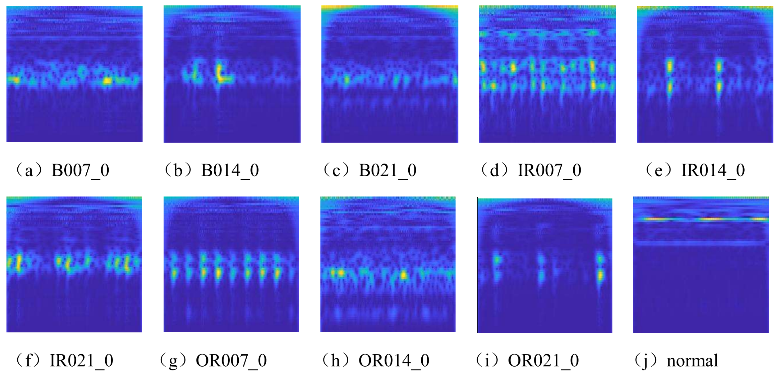
Considering the noise-resistant requirement of the model, the dataset selects the signal containing noise for experiments. The 2DCNN network as the benchmark model still has a classification accuracy of more than 99% on the noisy signal with SNR = −4, and the accuracy will decrease on the noisy signal with a lower signal-to-noise ratio. In order to ensure that the models participating in the experiment have a relatively high accuracy in the source domain so as to compare their domain adaptation capabilities, a noisy signal with SNR = −4 is selected for cross-domain experiments.
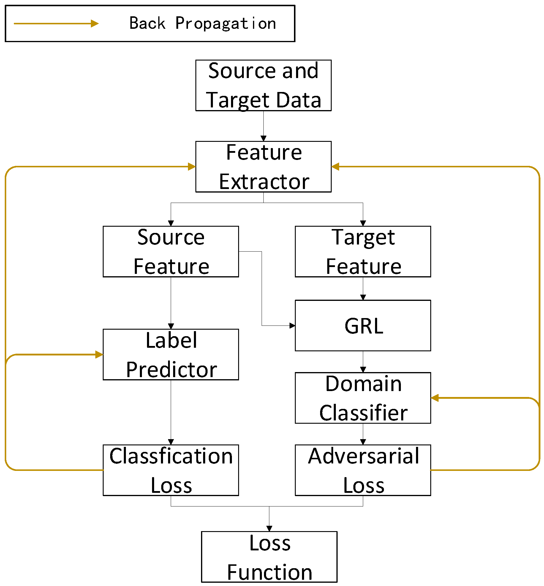
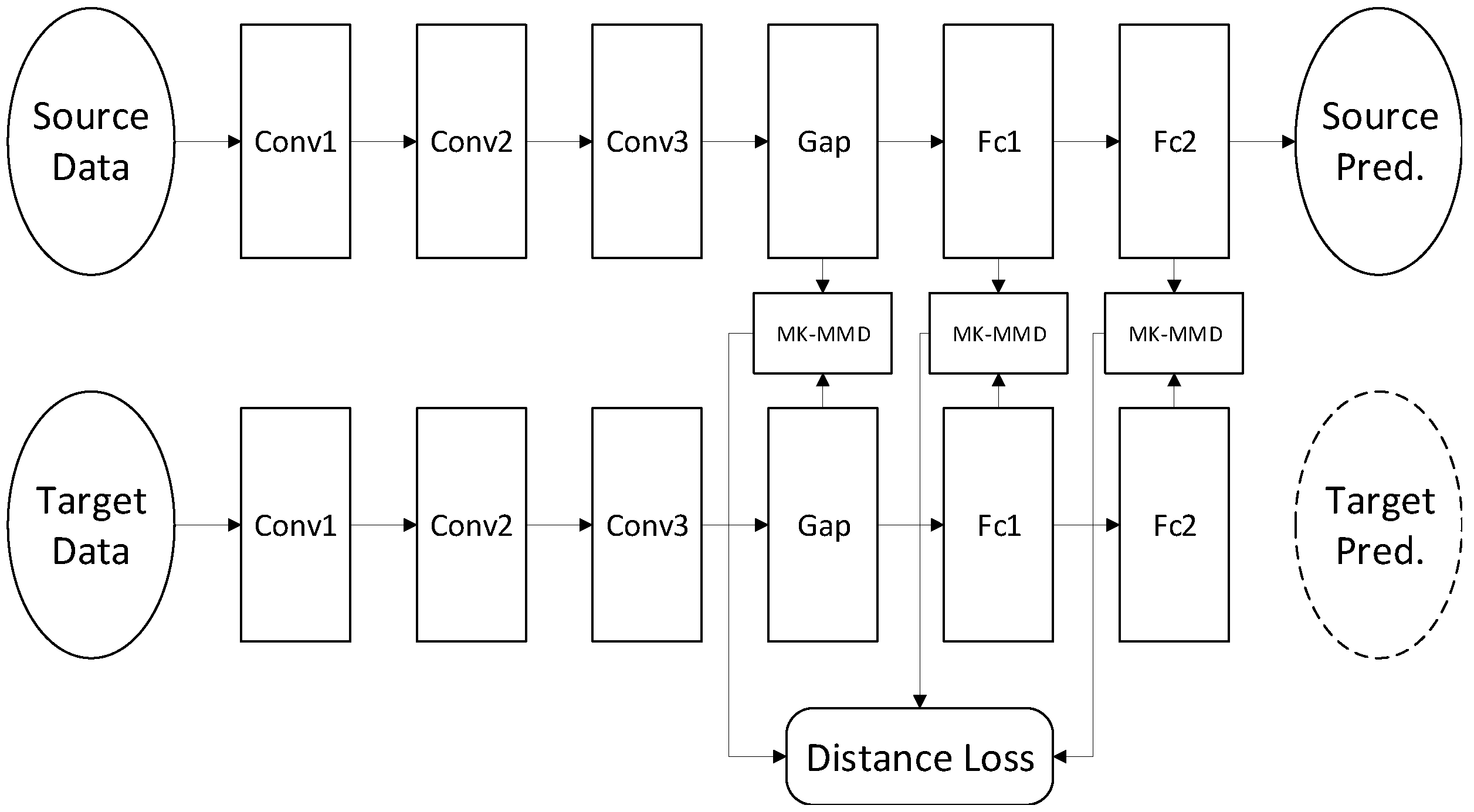
Among the methods for comparison, the classical CNN is first selected as the benchmark model to show the transfer performance of the model without any transfer method. Feature-based domain adaptation methods are then selected for comparison, represented by DAN using the MK-MMD distance and DSAN using the LMMD distance. In addition, adversarial-based domain adaptation methods are also selected for comparison, represented by DANN networks. The last is a composite model that combines the DANN and MK-MMD distance.
The classification accuracy of each method under cross-working conditions is shown in Table 2. The left side of the arrow represents the source domain, and the right side represents the target domain. The accuracy shown in the table is the classification accuracy of the model on the target domain. The accuracy on the source domain is close to 100%, so it is not shown in this table.
The results in Table 2 show that considering the CNN without any optimization and domain adaptation methods as the benchmark, the average accuracy of the CNN model on the unlabeled target domain is 87.08%.
However, DAN and DSAN, which use the distance method for domain adaptation, both perform mediocrely. DAN only outperforms the CNN model on a few cross-domain tasks, with no advantage in average accuracy. The DSAN method is even negative optimization, which is due to the fact that the image is filled with yellow areas representing noise signals, blurring the distribution between subfields and aligning non-identical sub-fields, resulting in negative optimization, while the use of the DANN network can improve the cross-domain accuracy to a certain extent. With an improvement of 3% to 4% in various cross-domain tasks, the average accuracy rate is increased to 91.57%. This result indicates that domain-invariant features can be found through adversarial training. On the basis of conversary, the composite model combined with the MK-MMD distance can further improve the cross-domain accuracy by 1% to 5%, indicating that the composite model combining these two methods can achieve a good classification result.
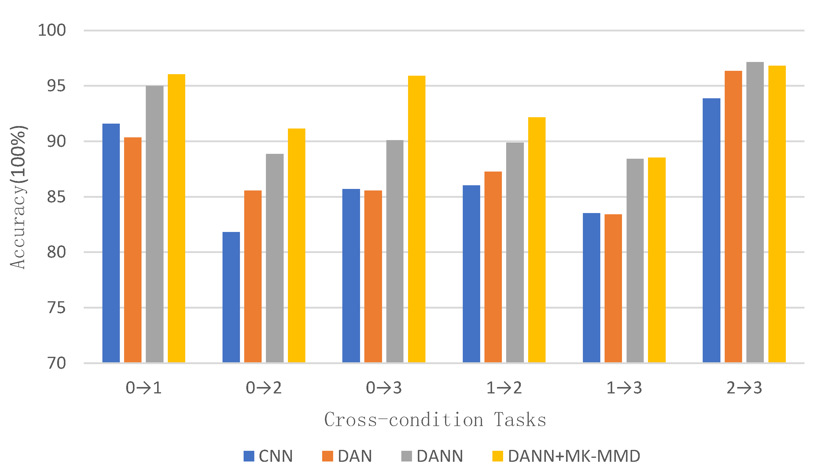
Figure 8 shows the accuracy result of the baseline CNN model, the feature-based DAN model, the adversarial-based DANN model, and the composite model.
It can be seen from Figure 8 that the composite model has high diagnosis accuracy on three cross-domain tasks of 0→1, 0→3, 2→3, all above 95%. On the cross-domain tasks of 0→2, 1→2, 1→3, The diagnosis accuracy is slightly lower, all around 90%. Compared with other methods, the composite model has the greatest improvement on the 0→3 cross-domain task, while the improvement in other cross-domain tasks is a bit smaller.
Although the composite model can improve the accuracy of diagnosis on various cross-domain tasks, the disadvantage of combining the two methods is that the model becomes bloated, and the loss function is complicated, resulting in a reduced training speed. This is where the composite model falls short.
Then this paper conducts multi-source domain adaptation experiments. The multi-source methods compared with the MCDANN method proposed in this paper fall into two categories. The first is the single-source domain optimal method. For each source domain, we use this method to operate a singe-source cross-domain test on the target domain and get the best accuracy as the benchmark accuracy. The second is the multi-source methods which are extended to single-source domain methods. Among the feature-based methods, the DAN method is selected for multi-source domain expansion, and the MK-MMD distance between each source domain and target domain is calculated and the weighted sum is performed as the domain loss function for training; Among the adversarial-based methods, the DANN method is selected for expansion, computing the adversarial loss between each source and a target domain and weighted summation as the domain loss function for training. The multi-source methods all take three source domains to participate in the training, and the comparison results of several methods are shown in Table 3.
Table 3 indicates that among the single-source domain methods, the composite model still has the best performance. Compared with the single-source domain, the DAN method and the DANN method using multi-source extension have a considerable improvement, which proves that multiple source domains can indeed provide more information to correct the problem of accuracy drop in cross-domain.
For the MCDANN method proposed in this paper, a consistency regularization loss is introduced besides the domain loss and classification loss, which improves the accuracy of the model by reducing the prediction difference on the target domain by models from several source domains. Therefore, we can get cross-domain diagnosis results in various domains with an accuracy of more than 96%, which proves its effectiveness.
However, the introduction of consistency loss also makes the loss function more complicated, thus affecting the speed of model training, making it slightly slower than other methods. This is also the disadvantage of MCDANN.
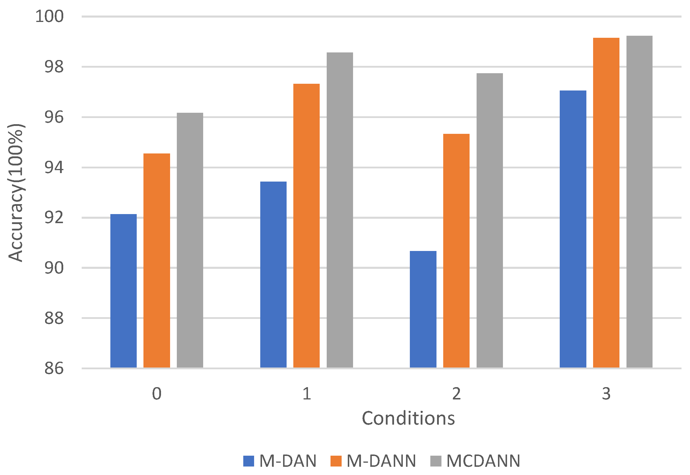
Figure 9 shows the accuracy comparison of several methods using multi-source domains under different working conditions. As can be seen from the figure, under the four unknown working conditions, the MCDANN method proposed in this paper has achieved the best accuracy. All these methods have lower accuracy on working conditions 0 and 2 and higher accuracy on 1 and 3. On working condition 3, since other methods have already achieved high diagnostic accuracy, the improvement of MCDANN is not large. On working condition 2, the MCDANN has the largest relative improvement.
In addition to the CWRU dataset, we also tested our model on DIRG bearing dataset. DIRG dataset is an open source dataset acquired on the rolling bearing test rig of the Dynamic and Identification Research Group (DIRG) from the Department of Mechanical and Aerospace Engineering at Politecnico di Torino [38]. This dataset includes a variety of speed and static load conditions, each with 6 failure modes, including two fault locations, inner ring or roller, each location includes 3 sizes of indentations, 450 um, 250 um, and 150 um. Due to the lack of some data, we decide to set the static load to 1000 N, and the rotational speed to 100 Hz, 200 Hz, 300 Hz, and 400 Hz as the four working conditions of No. 0~3 to carry out multi-source domain adaptive experiments. Except for the rotation speed as the working condition and these 6 fault modes as labels, other details are the same as the multi-source domain adaptation experiments on CWRU. The experimental results are shown as follows:
Table 4 and Figure 10 show that our model achieved the best accuracy on most cross-domain conditions except one when tested on the DIRG dataset without fine-tuning, indicating that it is not by chance that our model can achieve a good result, proving the effectiveness of our method.

4. Discussion

4.1. Ablation Study

To test the effect of the MK-MMD distance, a fault signal with SNR = −4 is used for experiments, and compare the performance of the original adversarial model and the model combined with different distance losses in cross-domain diagnosis. Each model is trained for 100 iterations. In each iteration, the training set of the source domain and the target domain is used for training, and then the model is applied to the test set from the source domain and the target domain to obtain the classification result. The test is repeated 10 times and obtains the average classification accuracy of the optimal accuracy from each time on the target domain as the classification result. As shown in Table 5, indices 0, 1, 2, and 3 represent the working conditions of the bearing under different loads, respectively, and the arrows indicate the direction of the cross-working condition.
As can be seen from Table 5, compared with the original adversarial network, the adversarial network that adds various distance metrics to correct the domain adversarial loss has a certain accuracy improvement, and the adversarial network that combines the MK-MMD distance has the best overall performance. However, the accuracy of adding MK-MMD distance is not so high. Due to the problem of domain mismatch, there are still different degrees of errors in cross-domain diagnosis.
Table 6 shows the result comparison of single-source and multi-source methods. In Table 6, for each domain, only one source domain is used for cross-domain diagnosis. We choose the optimal source domain cross-domain diagnosis result as the benchmark, which is compared with the result of dual-source domain MCDANN and triple-source domain MCDANN.
In this table, the accuracy improvement of MCDANN from dual-source domain to triple-source domain indicates that, as the number of source domains involved in training increases, the diagnostic accuracy of MCDANN will also improve.

4.2. Visualization Analysis

We performed Visual analysis of the model with confusion matrix and t-SNE [39] distribution. First, perform a visual analysis with the confusion matrix. We choose the composite model’s 0→2 cross-domain task with relatively lower accuracy for display. The visualization matrix of the results of applying the composite model to the test dataset from working condition 2 is shown in Figure 11a. It can be seen from the figure that the classification results of the composite model on the B021 fault have serious errors, and nearly 40% of the B021 faults are misclassified as B007 faults. Besides, 5.29% and 3.95% of the samples from the B007 fault and B014 fault were incorrectly classified as B021 fault, respectively, indicating that the composite model did not well distinguish the feature distributions corresponding to several fault diameters on the rolling ball. On the IR014 fault, 9.43% of the samples were incorrectly classified as the OR021 fault, indicating that the composite model could not completely classify the IR014 fault effectively. We believe that this is due to the phenomenon of domain mismatch because in this transfer, most of the classifications have achieved good results while only a few classes are seriously misclassified. The result indicates that the model incorrectly matches some B021 data of the target domain with the B007 data of the source domain, and calculates and reduces the field distribution between the two, so that this part of the B021 data is incorrectly classified as B007 data.
Then we show the confusion matrix of the results of applying MCDANN on the test set of working condition 2, as shown in Figure 11b. The classification accuracy of the MCDANN method on ball faults is generally low, and there are a few misclassifications between IR014 and OR021. However, although the misclassification problem of domain adaptation on ball faults cannot be completely solved, the MCDANN method still achieves a great improvement in this. On the B021 fault whose originally classification accuracy is 61.15%, the accuracy was increased to 92.55%, with an increase of more than 30%. Originally only 93.75% of B007 faults have been increased to 97.8%. The classification accuracy of the B007 fault is improved from 93.75% to 97.8% while the classification accuracy of B014 faults just has a slight improvement, from 95.39% to 95.97%.
Then the features obtained by these methods in the domain are visualized with t-SNE distribution, with working condition 0 as the source domain and working condition 2 as the target domain. Their t-SNE distribution of the feature from the last layer of the network is shown in Figure 12.
In this figure, the red part is the feature distribution of the target domain, that is, the distribution of the feature output of the last layer of the network on the test set of working condition 2. The gray part is the feature distribution of the source domain, that is, the output of the last layer of the network on the test set from working condition 0. The higher the degree of overlap between the two, the closer their domain distributions are. Since the domain adaptation model is trained on the labeled source domain, the prediction of the target domain is made according to the source domain label, so the prediction of the target domain can be judged by the degree of overlap between the gray area and the red area. For the convenience of observation, the gray area is placed on the upper layer, so that the degree of overlap between the two can be judged by observing the coverage of the gray area to the red area, and then the transfer performance of the model is analyzed accordingly.
Figure 12a is the result of the CNN model without any transfer method. It can be seen from the figure that the gray area is divided into 10 clusters, corresponding to the 10 fault modes in working condition 0. The distances between these gray clusters are not short, which indicates that the CNN model has successfully classified the data on the source domain. In the red area, there are only 8 clusters. In the upper right corner of the figure, we can see that there is a large red area covering two gray areas, indicating that two fault modes are confused together in the classification process of working condition 2, thus being classified into one cluster. On the right side of the figure, there is little overlap between the red area and the gray area, which indicates that there is a large distribution difference between the source and target domains on a specific fault mode. There is a gray area at the bottom of the figure with almost no red area overlapping with it, indicating that the CNN model hardly recognizes a certain fault in this working condition, so most samples of this fault are misclassified into other clusters. In other clusters, the gray area and the red area have some overlap, but they are not completely covered.
Figure 12b is the result of the composite domain adaptation model that combines the DANN network and the MK-MMD distance. It can be seen that the overall coverage of gray to red has improved, and each gray area covers the red area, indicating that the composite model improves the recognition rate of faults in working condition 2, and faults can be successfully classified into 10 categories. However, there are still only 9 red clusters, and there is still a large red area connected together in the upper left corner, indicating that the two confused faults have not been effectively distinguished.
Figure 12c is the result of the MCDANN model using a multi-source domain for domain adaptation. In the final feature output of the model, it can be seen that the gray coverage is quite high, and the red part that can be seen in the figure is the least. Not only the gray area can be divided into 10 clusters, but the red area can also be roughly divided into 10 clusters. Although there are two red areas on the left that are still connected, it is much better than the connected red areas in (a) and (b). This shows that the MCDANN model performs well on the unlabeled test set from working condition 2, which also proves the effectiveness of the method proposed in this paper.

5. Conclusions and Future Work

This paper proposes a multi-source consistency domain adaptation model MCDANN that can adapt the fault diagnosis model to other unknown working conditions. MCDANN is based on the domain adversarial network, using the MK-MMD distance to further reduce the difference between the source domain and the target domain in the feature space, and using sub-domain alignment and multi-source domain adaptation methods to perform more fine-grained matching in the domain to solve the domain Mismatch problem. On the CWRU data set, experiments are carried out using the noisy fault data set with a signal-to-noise ratio of −4. The experiments show that the MCDANN can achieve an accuracy rate of more than 96% under various unknown working conditions, which is better than other adaptation methods.
The current experiments are only carried out on the bearing dataset. If more fault datasets containing domains can be obtained, the optimization of the existing model can undoubtedly go further. In addition, the current method has many ideal preconditions, such as the same number of labels in the source and target domains, and the source domain has many and abundant data. Compared with the experimental conditions, the actual situation is undoubtedly much more complicated, and this is also a direction that can be further expanded, such as small sample learning, local domain adaptation, etc. On the other hand, domain adaptation methods usually need to access the target domain data. Although the target domain data has no labels, the information contained in the target domain data itself is enough for the model to learn enough knowledge to complete the domain transfer. However, if one or more source domain data can be used for training to obtain a model with excellent performance without accessing the target domain data in the unknown domain, it is undoubtedly more practical work, which is also an extension of the domain adaptation problem and domain generalization problem.

Author Contributions

Funding acquisition, H.C.; methodology, H.C.; software, L.S. and S.Z.; validation, L.S. and S.Z.; formal analysis, H.C., Y.Y., and N.A.; investigation, L.S., S.Z., and Y.Y.; resources, H.C.; data curation, L.S. and Y.Y.; writing—original draft, L.S. and S.Z.; supervision, H.C.; project administration, H.C. and N.A.; writing—review and editing, Y.Y. and N.A. All authors have read and agreed to the published version of the manuscript.

Funding

This research was funded by the China National Key R&D Program during the 13th Five-year Plan Period (Grant No. 2018YFB1700405).

Institutional Review Board Statement

Not applicable.

Informed Consent Statement

Not applicable.

Data Availability Statement

Publicly available datasets were analyzed in this study. This data can be found here: https://engineering.case.edu/bearingdatacenter/download-data-file (accessed on 2 March 2021).

Conflicts of Interest

The authors declare no conflict of interest.

Nomenclature

CNNconvolutional neural network
DAEdeep auto-encoder
SDAstacked denoising autoencoder
DANN      domain-adversarial training of neural networks
MMDmaximum mean discrepancy
MK-MMDmulti-kernels maximum mean discrepancy
WDCNNdeep convolutional neural networks with wide first-layer kernel
AdaBNadaptive batch normalization
DSANdeep subdomain adaption network
MCDANNmulti-source consistency domain adaptation neural network
G f feature extractor
G y label classifier
G d domain classifier
L y difference between the prediction of the label classifier and the real label
L d difference between the predicted domain and the real domain
Ffunction domain
fa function belonging to the function domain F
H k the RKHS obtained by a feature kernel k
β u the weight of kernel u

References

  1. Zhang, S.; Zhang, S.; Wang, B.; Habetler, T.G. Deep learning algorithms for bearing fault diagnostics—A comprehensive review. IEEE Access 2020, 8, 29857–29881. [Google Scholar] [CrossRef]
  2. Luo, Z.; Wang, J.; Tang, R.; Wang, D. Research on vibration performance of the nonlinear combined support-flexible rotor system. Nonlinear Dyn. 2019, 98, 113–128. [Google Scholar] [CrossRef]
  3. Zhang, Y.; Li, X.; Gao, L.; Wang, L.; Wen, L. Imbalanced data fault diagnosis of rotating machinery using synthetic oversampling and feature learning. J. Manuf. Syst. 2018, 48, 34–50. [Google Scholar] [CrossRef]
  4. Gao, Z.; Cecati, C.; Ding, S.X. A survey of fault diagnosis and fault-tolerant techniques—part i: Fault diagnosis with model-based and signal-based approaches. IEEE Trans. Ind. 2015, 62, 3757–3767. [Google Scholar] [CrossRef] [Green Version]
  5. Yang, Z.; Gjorgjevikj, D.; Long, J.; Zi, Y.; Zhang, S.; Li, C. Sparse autoencoder-based multi-head deep neural networks for machinery fault diagnostics with detection of novelties. Chin. J. Mech. Eng. 2021, 34, 1–12. [Google Scholar] [CrossRef]
  6. Li, H.; Bu, S.; Wen, J.-R.; Fei, C.-W. Synthetical modal parameters identification method of damped oscillation signals in power system. Appl. Sci. 2022, 12, 4668. [Google Scholar] [CrossRef]
  7. Tian, J.; Yi, G.-W.; Fei, C.-W.; Zhou, J.; Ai, Y.-T.; Zhang, F.-L. Quantum entropy-based hierarchical strategy for inter-shaft bearing fault detection. Struct. Control. Health Monit. 2021, 28, e2839. [Google Scholar] [CrossRef]
  8. Tian, J.; Liu, L.; Zhang, F.; Ai, Y.; Wang, R.; Fei, C. Multi-domain entropy-random forest method for the fusion diagnosis of inter-shaft bearing faults with acoustic emission signals. Entropy 2019, 22, 57. [Google Scholar] [CrossRef] [Green Version]
  9. Tian, J.; Wang, S.-G.; Zhou, J.; Ai, Y.-T.; Zhang, Y.-W.; Fei, C.-W. Fault diagnosis of intershaft bearing using variational mode decomposition with taga optimization. Shock Vib. 2021, 2021, 8828317. [Google Scholar] [CrossRef]
  10. Munikoti, S.; Das, L.; Natarajan, B.; Srinivasan, B. Data-driven approaches for diagnosis of incipient faults in dc motors. IEEE Trans. Ind. Inform. 2019, 15, 5299–5308. [Google Scholar] [CrossRef]
  11. Wang, H.; Xu, J.; Yan, R.; Gao, R.X. A new intelligent bearing fault diagnosis method using sdp representation and se-cnn. IEEE Trans. Instrum. Meas. 2019, 69, 2377–2389. [Google Scholar] [CrossRef]
  12. Guo, L.; Lei, Y.; Li, N.; Xing, S. Deep convolution feature learning for health indicator construction of bearings. In Proceedings of the 2017 Prognostics and System Health Management Conference (PHM-Harbin), Harbin, China, 9–12 July 2017; pp. 1–6. [Google Scholar]
  13. Chen, Y.; Peng, G.; Xie, C.; Zhang, W.; Li, C.; Liu, S. Acdin: Bridging the gap between artificial and real bearing damages for bearing fault diagnosis. Neurocomputing 2018, 294, 61–71. [Google Scholar] [CrossRef]
  14. Qian, W.; Li, S.; Wang, J.; An, Z.; Jiang, X. An intelligent fault diagnosis framework for raw vibration signals: Adaptive overlapping convolutional neural network. Meas. Sci. Technol. 2018, 29, 095009. [Google Scholar] [CrossRef]
  15. Chen, Z.; Li, W. Multisensor feature fusion for bearing fault diagnosis using sparse autoencoder and deep belief network. IEEE Trans. Instrum. Meas. 2017, 66, 1693–1702. [Google Scholar] [CrossRef]
  16. Guo, J.; Zheng, P. A method of rolling bearing fault diagnose based on double sparse dictionary and deep belief network. IEEE Access 2020, 8, 116239–116253. [Google Scholar] [CrossRef]
  17. Zou, Y.; Zhang, Y.; Mao, H. Fault diagnosis on the bearing of traction motor in high-speed trains based on deep learning. Alex. Eng. J. 2021, 60, 1209–1219. [Google Scholar] [CrossRef]
  18. Surendran, R.; Khalaf, O.I.; Andres, C. Deep learning based intelligent industrial fault diagnosis model. CMC-Comput. Mater. Contin. 2022, 70, 6323–6338. [Google Scholar] [CrossRef]
  19. Arellano-Espitia, F.; Delgado-Prieto, M.; Gonzalez-Abreu, A.-D.; Saucedo-Dorantes, J.J.; Osornio-Rios, R.A. Deep-compact-clustering based anomaly detection applied to electromechanical industrial systems. Sensors 2021, 21, 5830. [Google Scholar] [CrossRef]
  20. Li, X.; Zhang, W.; Ding, Q. Understanding and improving deep learning-based rolling bearing fault diagnosis with attention mechanism. Signal Process. 2019, 161, 136–154. [Google Scholar] [CrossRef]
  21. Wang, H.; Xu, J.; Yan, R.; Sun, C.; Chen, X. Intelligent bearing fault diagnosis using multi-head attention-based cnn. Procedia Manuf. 2020, 49, 112–118. [Google Scholar] [CrossRef]
  22. Yao, Y.; Zhang, S.; Yang, S.; Gui, G. Learning attention representation with a multi-scale cnn for gear fault diagnosis under different working conditions. Sensors 2020, 20, 1233. [Google Scholar] [CrossRef] [PubMed] [Green Version]
  23. Jiao, J.; Zhao, M.; Lin, J.; Liang, K. A comprehensive review on convolutional neural network in machine fault diagnosis. Neurocomputing 2020, 417, 36–63. [Google Scholar] [CrossRef]
  24. Zhang, S.; Lei, S.; Jiefei, G.; Ke, L.; Lang, Z.; Pecht, M. Rotating machinery fault detection and diagnosis based on deep domain adaptation: A survey. Chin. J. Aeronaut. 2021. [Google Scholar] [CrossRef]
  25. Zhang, Z.; Chen, H.; Li, S.; An, Z. Unsupervised domain adaptation via enhanced transfer joint matching for bearing fault diagnosis. Measurement 2020, 165, 108071. [Google Scholar] [CrossRef]
  26. Deng, M.; Deng, A.; Zhu, J.; Shi, Y.; Liu, Y. Intelligent fault diagnosis of rotating components in the absence of fault data: A transfer-based approach. Measurement 2021, 173, 108601. [Google Scholar] [CrossRef]
  27. Zhu, J.; Chen, N.; Shen, C. A new deep transfer learning method for bearing fault diagnosis under different working conditions. IEEE Sens. J. 2019, 20, 8394–8402. [Google Scholar] [CrossRef]
  28. Che, C.; Wang, H.; Ni, X.; Fu, Q. Domain adaptive deep belief network for rolling bearing fault diagnosis. Comput. Ind. Eng. 2020, 143, 106427. [Google Scholar] [CrossRef]
  29. Wang, Q.; Michau, G.; Fink, O. Domain adaptive transfer learning for fault diagnosis. In Proceedings of the 2019 Prognostics and System Health Management Conference (PHM-Paris), Paris, France, 2–5 May 2019; pp. 279–285. [Google Scholar]
  30. Jiao, J.; Lin, J.; Zhao, M.; Liang, K. Double-level adversarial domain adaptation network for intelligent fault diagnosis. Knowl.-Based Syst. 2020, 205, 106236. [Google Scholar] [CrossRef]
  31. Li, X.; Zhang, W.; Ma, H.; Luo, Z.; Li, X. Deep learning-based adversarial multi-classifier optimization for cross-domain machinery fault diagnostics. J. Manuf. Syst. 2020, 55, 334–347. [Google Scholar] [CrossRef]
  32. Guo, L.; Lei, Y.; Xing, S.; Yan, T.; Li, N. Deep convolutional transfer learning network: A new method for intelligent fault diagnosis of machines with unlabeled data. IEEE Trans. Ind. Electron. 2018, 66, 7316–7325. [Google Scholar] [CrossRef]
  33. Li, X.; Zhang, W.; Ma, H.; Luo, Z.; Li, X. Domain generalization in rotating machinery fault diagnostics using deep neural networks. Neurocomputing 2020, 403, 409–420. [Google Scholar] [CrossRef]
  34. Zhao, K.; Jiang, H.; Wang, K.; Pei, Z. Joint distribution adaptation network with adversarial learning for rolling bearing fault diagnosis. Knowl.-Based Syst. 2021, 222, 106974. [Google Scholar] [CrossRef]
  35. Zhang, W.; Peng, G.; Li, C.; Chen, Y.; Zhang, Z. A new deep learning model for fault diagnosis with good anti-noise and domain adaptation ability on raw vibration signals. Sensors 2017, 17, 425. [Google Scholar] [CrossRef] [Green Version]
  36. Zhu, Y.; Zhuang, F.; Wang, J.; Ke, G.; Chen, J.; Bian, J.; Xiong, H.; He, Q. Deep subdomain adaptation network for image classification. IEEE Trans. Neural Netw. Learn. Syst. 2020, 32, 1713–1722. [Google Scholar] [CrossRef]
  37. Ganin, Y.; Ustinova, E.; Ajakan, H.; Germain, P.; Larochelle, H.; Laviolette, F.; Marchand, M.; Lempitsky, V. Domain-adversarial training of neural networks. J. Mach. Learn. Res. 2016, 17, 2096–2130. [Google Scholar]
  38. Daga, A.P.; Fasana, A.; Marchesiello, S.; Garibaldi, L. The politecnico di torino rolling bearing test rig: Description and analysis of open access data. Mech. Syst. Signal Process. 2019, 120, 252–273. [Google Scholar] [CrossRef]
  39. der Maaten, L.V.; Hinton, G. Visualizing data using t-SNE. J. Mach. Learn. Res. 2008, 9, 2008. [Google Scholar]
Figure 1. MCDANN architecture.
Applsci 12 10113 g001
Figure 2. DANN training process.
Applsci 12 10113 g002
Figure 3. Application of MK-MMD distance.
Applsci 12 10113 g003
Figure 4. Schematic diagram of Domain Adaptation.
Applsci 12 10113 g004
Figure 5. Single-source domain adaptation and multi-source domain adaptation.
Applsci 12 10113 g005
Figure 6. Network structure of the feature extractor, label classifier and domain classifier in MCDANN. (a) Feature Extractor; (b) Label Classifier; (c) Domain Classifier.
Applsci 12 10113 g006
Figure 7. Wavelet transform images of different fault modes under load condition 0.
Applsci 12 10113 g007
Figure 8. Classification accuracy of each method under cross-working conditions.
Applsci 12 10113 g008
Figure 9. CWRU classification accuracy comparasion of three multi-source domain adaptation models on unknown working conditions without labels (SNR = −4).
Applsci 12 10113 g009
Figure 10. DIRG classification accuracy comparison of three multi-source domain adaptation models on unknown working conditions without labels. (SNR = −4, static load = 1000 N).
Applsci 12 10113 g010
Figure 11. Confusion matrix of single source model and multi-source model on working condition 2. (SNR = −4). (a) DANN+MK-MMD; (b) MCDANN.
Applsci 12 10113 g011
Figure 12. Different models’ domain distribution output of the test set from working condition 2. (SNR = −4). (a) CNN; (b) DANN+MK-MMD; (c) MCDANN.
Applsci 12 10113 g012
Table 1. CWRU bearing dataset.
Fault IndicesFault PositionFault DiagramLoad (HP)
0123
1 0.007B007_0B007_1B007_2B007_3
2Ball0.014B014_0B014_1B014_2B014_3
3 0.021B021_0B021_1B021_2B021_3
4 0.007IR007_0IR007_1IR007_2IR007_3
5Inner raceway0.014IR014_0IR014_1IR014_2IR014_3
6 0.021IR021_0IR021_1IR021_2IR021_3
7 0.007OR007_0OR007_1OR007_2OR007_3
8Outer raceway0.014OR014_0OR014_1OR014_2OR014_3
9 0.021OR021_0OR021_1OR021_2OR021_3
0Normal normal_0normal_1normal_2normal_3
Table 2. Cross-domain classification accuracy of different models.
ModelCross-Working ConditionAverage
0→10→20→31→21→32→3
CNN91.5981.8285.6886.0283.5293.8687.08
DAN90.3485.5785.5787.2783.4196.3688.09
DSAN85.1178.2380.3483.4178.5291.4787.08
DANN95.0088.8690.1189.8788.4197.1591.57
DANN+MK-MMD96.0291.1395.9192.1688.5296.8193.43
Note: The bold number mean it is the largest in this column.
Table 3. CWRU classification accuracy of different models on unknown working condition without labels. (SNR = −4).
ModelDomainAverage
0123
Single DAN86.1590.3487.2796.3690.03
Single DANN90.329589.8797.1593.09
Single DANN+MK-MMD93.1596.0292.1696.8794.55
Multi DAN92.1493.4390.6797.0593.32
Multi DANN94.5497.3295.3399.1596.59
MCDANN96.1798.5697.7499.2397.93
Note: The bold number mean it is the largest in this column.
Table 4. DIRG classification accuracy of different models on unknown working conditions without labels. (SNR = −4, static load = 1000 N).
ModelDomainAverage
0123
Multi DAN95.5193.4096.3793.2194.62
Multi DANN98.4592.1593.6695.4894.93
MCDANN98.4992.0298.5195.8196.20
Note: The bold number mean it is the largest in this column.
Table 5. Classification accuracy of models using distance for domain adaptation in cross-working conditions.
ModelCross-Working ConditonAverage
0→10→20→31→21→32→3
DANN9588.8690.1189.8788.4197.1591.57
DANN+MMD96.3190.1793.2291.2488.3396.3492.6
DANN+MK-MMD96.0291.1395.9192.1688.5296.8193.43
Note: The bold number mean it is the largest in this column.
Table 6. Classification accuracy of cross-domain models with different number of source domains under cross-working conditions.
ModelWorking ConditionsAverage
0123
MK-MMD+DANN93.1596.0292.1696.8794.55
Dual source domains MCDANN94.6798.1794.5498.3596.48
Three source domains MCDANN96.1798.5697.7499.2397.93
Note: The bold number mean it is the largest in this column.
Publisher’s Note: MDPI stays neutral with regard to jurisdictional claims in published maps and institutional affiliations.

