A High-Precision Method for Evaluating Sector Capacity in Bad Weather Based on an Improved WITI Model

Abstract

The rapid development of the civil aviation industry has increased the pressure on airspace resources in China. The traditional sector capacity assessment method does not take into account the impact of bad weather, resulting in flight plans often deviating markedly from the predicted plans, causing flight delays and affecting the punctuality rate of flights. To solve this issue, we propose a novel evaluation method based on an improved Weather-Impacted Traffic Index (WITI) model to calculate sector capacity. The WITI model is optimized in order to calculate the weather-influence coefficients under different types of bad weather. These coefficients were also considered in a controller workload model. Finally, the model was trained using a deep-neural-network algorithm, which is combined with a linear regression algorithm to calculate sector capacity under different bad weather conditions. The novel approach leads to the output results being within a specified error range, which greatly improves their accuracy. This method was applied to the actual case data of Yinchuan Hedong International Airport to consider different types of bad weather and quantify their severity, which more specifically assesses the sector capacity under the condition of bad weather.

1. Introduction

The rapid development of civil aviation is resulting in increased air traffic flows. In order to correctly manage air traffic and also improve its efficiency and safety, a method for reliably evaluating sector capacity has recently become a focus of research. According to statistics, the most serious factor affecting the flight irregularity rate in 2019 was weather [1]. Bad weather can greatly reduce the ability of a sector to accommodate flights, and flights in the affected airspace often choose to divert, detour, or return in order to avoid adverse outcomes [2]. All of these factors increase the workload of air traffic controllers and flight delays, and in broader terms, seriously affect the development of the civil aviation transportation industry [3]. Therefore, evaluating the sector capacity based on bad weather is both necessary and meaningful.

Sector capacity has been studied since 1970. Janic and Tosic established a simple mathematical model that took into account the sector structure of the airspace, traffic flow characteristics, and control rules [4]. The initial research into sector capacity only involved theoretical analyses. The gradual development of the civil aviation industry has increased the required airspace capacity [5], and more scholars are now studying practical sector capacities. Tofukuji predicted the maximum capacity at Tokyo Airport in the actual operating environment by analyzing whether the controller’s workload was the limiting factor of capacity [6,7], which enhanced the practicality of capacity assessments.

Developments in machine learning are allowing neural network algorithms to be used to improve controller workload evaluation models and thereby also the accuracy of workload evaluations [8]. Amitabh develops GEOSECT software that assesses controller workload and assists in the delineation of control sectors based on GEOSECT assessments [9]. In the same year, a sector capacity evaluation model based on the complexity of the airspace established using the k-means algorithm divided the workload of the controller into radar and non-radar control work [10]. Yang divided the controller workload into four types based on static sector coupling and dynamic sector coupling: background load, base load, cyclic load, and conflict load, and obtained an improved four-element controller workload model under the condition of multisector coupled operation [11]. Aiming at the problem that sector capacity assessment is independent of each other, Li gave a capacity assessment method under the condition of sector coupling [12].

Most of the popular control sector capacity assessment methods consider only the controller’s speech, operation, and cognitive load. Moreover, current sector capacity evaluation models only include the number of aircrafts that can be accommodated in a sector under normal circumstances, and rarely consider the influence of the weather. There are a few methods for quantitatively describing the influence of weather on sector capacity, but they are difficult to use as a reference factor for sector capacity evaluation. In 2011, RA used the airway convective weather avoidance model to convert the airspace that the aircraft could not pass into the weather avoidance area, and then used the airway congestion algorithm to calculate the flow control area. Then the simple average method is used to converge into the blockage of a single flow control area. The capacity of the flow control area is defined as: a 100-blocking value, which provides a new idea for the prediction of sector dynamic capacity under bad weather [13]. Chen proposed a new algorithm to solve the uncertainty problem of airport capacity under bad weather by using the opportunity-constrained optimization method. Based on the existing deterministic integer programming optimization model of airport capacity under bad weather, he established a chance-constrained model that includes probabilistic sector capacity constraints. Then, in order to effectively solve such a large-scale opportunity-constrained optimization problem, a method based on polynomial approximation is adopted [14].

The FAA established the Weather-Impacted Traffic Index (WITI) concept and model in 2004 based on live weather information and traffic demand, and this was developed by the MITRE company to measure the impact of weather on traffic flow in the US national airspace system. The WITI is widely used in airspace capacity predictions, and representative prediction models include capacity prediction using WITI based on traffic flow, predictive analysis of WITI and flight delays, and capacity prediction methods using WITI to build scenario trees [15]. However, the classic WITI model only includes the impact of weather on sector capacity under the influence of thunderstorms. In actual operation, there are many other types of bad weather conditions that affect flight operations, and these different types of bad weather will affect sector capacity to varying degrees. In 2019, Zhang proposed a multi-sector dynamic capacity evaluation method to solve the problem that the existing capacity evaluation technology is not comprehensive enough. Through the concept of sector-capacity influencing factors and sector coupling, a workload model of the multi-sector controller was established. Then, by quantifying the degree of congestion of the airspace unit, the availability of multiple sectors in severe weather is obtained [16].

This paper proposes a new method to address this problem. We use a modified WITI model to take into account different types of bad weather in the capability assessment and identify and quantify the effects. This is then added as a variable to the controller’s workload model, which is trained using the DNN (deep neural network) algorithm to obtain more accurate predictions of the sector capacity. This approach leads to the output results being within a specified error range, which greatly improves their accuracy. In short, this new method takes into account different types of bad weather, quantifies their severity, and, more specifically, assesses the sector capacity under the condition of bad weather.

The remainder of this paper is organized as follows: Section 2 optimizes the WITI model based on the Gaussian mixture clustering algorithm, classifies different types of bad weather according to different intensities of meteorological radar echoes, and calculates the weather-influence coefficient. Section 3 adopts the DNN algorithm, with input variables such as the selected sector flow, the number of commands, the command duration, the optimized weather-influence coefficient, and the number of diverted flights used to generate the controller workload as the output, so as to obtain a more accurate prediction of the sector capacity. Section 4 presents numerical calculations and simulation experiments. Finally, conclusions are drawn and ideas for further work are proposed in Section 5.

The architecture diagram of the overall system is shown in Figure 1.

2. Improved WITI Model Considering Gaussian Mixture Clustering

2.1. Gaussian Mixture Clustering

The finite mixture model (FMM) is a method in which a complex density distribution is assessed by combining multiple simple distributions. Based on the FMM, the Gaussian mixture model is obtained by limiting all distributions to the Gaussian distribution [17].

We first perform a cluster analysis of bad weather. It is assumed that sample set $D=\{x_1,x_2,\dots ,x_n\}$ contains $n$ unlabeled samples. Each sample $x_i=\{x_{i1};x_{i2};\dots ;x_{im}\}$ is a m-dimension feature vector containing echo intensity and weather data information. The clustering algorithm divides sample D into k clusters $\left\{C_l\right|l=1,2,\dots ,k\}$, where $C_{l^{\prime }}{\cap }_{l^{\prime }\ne l}{C}_l=\varnothing$ and $D={\cup }_{l=1}^k{C}_l$. Accordingly, $a_j\in \{1,2,\dots ,k\}$ is used to represent the “cluster mark” of sample $x_j$, $x_j\in C_{aj}$. Therefore, the clustering result can be represented by a cluster label vector $\overrightarrow{a}=\{a_1;a_2;\dots ;a_n\}$ containing n elements; this represents the final classification result of bad-weather types.

The specific calculation formula is as follows:

$$P(x)={\displaystyle \sum _{i=1}^k{\lambda }_{i}p\left(x|{\mu }_i,{\displaystyle \sum i}\right)},i=\{1,2,\dots ,k\}$$

(1)

where x is the vector in sample space D (i.e., echo intensity and weather phenomenon data), ${\lambda }_i$ is the mixing coefficient, and $P(x|u_i,\sum i)$ is the $i$-th Gaussian distribution that both points to $u_i$ and covariance $\sum i$:

$$p(x|{\mu }_i,{\displaystyle \sum i})=\frac{\exp [-1/2{(x-{\mu }_i)}^{T{\displaystyle {\sum }_i^{-1}(x-{\mu }_i)}}}{{(2\pi )}^{n/2}{\left|{\displaystyle \sum i}\right|}^{1/2}}$$

(2)

If the values of parameters ${\lambda }_i$, $u_i$, ${\displaystyle \sum i}$, and i are determined, Equation (2) can be used to obtain the probability $P(x|u_i,{\displaystyle \sum i})$ of each Gaussian component generating sample X and density $p(x)$ of the Gaussian mixture distribution.

Let sample data set j be used to calculate the probability that the Gaussian component of generated sample $x_n$ according to the Bayesian theorem, and record the largest Gaussian component of ${\gamma }_{nj}$ as the category of $x_n$. This is based on the principle of Gaussian mixture clustering.

The parameter estimation takes the maximum-likelihood estimation as the optimization objective and uses the expectation maximization algorithm to solve the problem [18]. The initial parameters of Gaussian mixture clustering are set, and the posterior probability ${\gamma }_{nj}$ that sample $x_n$ a belongs to Gaussian component j is calculated using the current parameters:

$$\begin{gathered} {\gamma }_{nj}=p(c_n=j|x_n) \\ =\frac{p(c_n=j)p(x|{\mu }_i,j)}{P(x_n)} \\ =\frac{{\lambda }_{i}p(x_n|{\mu }_j,{\displaystyle \sum j})}{{\displaystyle \sum _{i=1}^k{\lambda }_{i}p(x|{\mu }_i,{\displaystyle \sum i})}} \end{gathered}$$

(3)

Mean ${\mu }_j$ and covariance ${\displaystyle \sum j}$ are calculated as

$${\lambda }_i=\frac{1}{N}{\displaystyle \sum _{n=1}^N{\gamma }_{nj}}$$

(4)

$${\mu }_j=\frac{{\displaystyle \sum _{n=1}^N{\gamma }_{nj}{X}_n}}{{\displaystyle \sum _{n=1}^N{\gamma }_{nj}}}$$

(5)

$${\displaystyle \sum j=\frac{{\displaystyle \sum _{n=1}^N{\gamma }_{nj}(x_n-x_j){(x_n-{\mu }_j)}^T}}{{\displaystyle \sum _{n=1}^N{\gamma }_{nj}}}}$$

(6)

The clustering results are then obtained by iterating to convergence.

The Gaussian mixture clustering model can be used to classify bad weather in the sector according to the echo intensity and weather phenomenon. By inputting the sample data of the echo intensity and weather types in the sector, the bad weather is combined with the WITI model to measure the severity of the bad weather according to the echo intensity, so as to realize the classification of bad weather and calculate different weather types. The influence of bad weather on sector capacity can be quantified by using the weather-influence coefficient according to different categories.

2.2. Improved WITI Model

The WITI has been used to measure the impact of weather on the traffic flow of the national airspace system of the US, which has demonstrated that it is suitable for large-scale and long-term weather impact analyses [19].

In the original WITI model, the sector airspace within the research scope is divided into several very small areas using a grid, where each area is a computing unit. It is assumed that the sector airspace network has m rows and N columns, and the grid of the $i$-th row and $j$-th column is denoted as grid $ij$. This approach means that the continuous sector airspace system is discretized into grid points.

The weather information and traffic flow information in the grid are calculated and superimposed on the research sector airspace system. The weather information on grid $ij$ is recorded as $W_{ij}$, and the traffic flow information is recorded as $T_{ij}$. Initially, weather information refers to severe convective weather, which can be identified and gridded on the weather radar. Traffic flow information refers to the number of flights passing through the grid during the $t$-th time period. Based on the WITI model, the value of WITI ($k$) during the $k$-th time period is

$$\mathrm{WITI}(t)={\displaystyle \sum _{i=1}^m{\displaystyle \sum _{j=1}^n{T}_{ij}(t)W_{ij}(t)}}$$

(7)

Traffic flow information $T_{ij}$ in the model refers to the number of aircraft flying through grid $ij$ during the $t$-th time period of the reference weather, while weather information $W_{ij}(t)$ is a Boolean variable:

$$W_{ij}(t)=\{\begin{array}{l}0, grid\hspace{1em}ij has no bad weather during time period\hspace{1em}t\\ 1, grid\hspace{1em}ij has bad weather during time period\hspace{1em}t\end{array}$$

The classical WITI model can only be used to calculate the effect of thunderstorm weather on the sector capacity, in terms of the number of flights. However, in the actual situation, there are many types of bad weather conditions that affect flight operation; that is, this is not limited to thunderstorm weather. This problem is addressed by using a Gaussian mixture clustering model to optimize the situation. According to the clustering results, the bad weather is classified according to the echo intensity, and bad weather of type $a$ is obtained. By calculating the weather-influence coefficient $W_{ij,a}(t)$ under different bad weather conditions, the optimized WITI model is obtained:

$${\mathrm{WITI}}^{\prime }(t)={\displaystyle \sum _{i=1}^m{\displaystyle \sum _{j=1}^n{T}_{ij}(t)W_{ij,a}(t)}}$$

(8)

$$W_{ij,a}(t)=\frac{F_{ij}^{\prime }(t)}{F_{p,ij}(t)}$$

(9)

where $F_{ij}^{\prime }(t)$ is the number of affected aircraft and $F_{p,ij}(t)$ is the number of scheduled flights during the $t$-th time of grid $ij$.

3. Sector Capacity Evaluation Method Based on the DNN Algorithm

3.1. Route-Availability Model

The route-availability model is first used to identify the flights that need to be rerouted due to bad weather in the sector. When the aircraft enters the control sector, rerouting, returning, and forced landing will occur due to the weather. Resolving conflicts between the rerouted aircraft requires the controller to issue multiple instructions to adjust flight plans, which will increase the workload of the controller. In addition, the capacity of the sector changes. The main task in this section is to statistically calculate the number of rerouted aircraft under different types of bad weather conditions so that the corresponding sector capacities can be calculated.

According to the theory of maximum flow and minimum cut, when the directions of the traffic flow in a plane are the same, the maximum flow that can pass in that plane is not based on the average value, but instead determined by the flow that can pass through the narrowest place in the plane, that is, the plane bottleneck. Therefore, according to the theory, it can be assumed that route $L$ is connected to $K$ rectangular regions at altitude level $I$, and the blocking probability of route $l$ at this altitude is determined by the rectangle with the largest blocking value among the $K$ rectangular regions [20]. Thus, the blocking probability of route $l$ at altitude level $I$ can be obtained as

$$q_{}^{Li}=\underset{1\le D\le k}{\max }{q}_D^{Li}$$

(10)

where $q_{}^{Li}$ is the blocking probability of route $L$ at altitude level $i$.

If there are m available altitude levels on route $L$, the blocking probability of route $L$ under the influence of bad weather can be expressed as

$$\begin{gathered} q^L={\displaystyle \sum _{i=1}^M{q}^{Li}}/M \\ ={\displaystyle \sum _{i=1}^M(\underset{1\le D\le k}{\max }{q}_D^{Li}})/M \\ ={\displaystyle \sum _{i=1}^M\underset{1\le D\le k}{\max }\left[{\displaystyle \sum _{n=1}^{32}\left(\frac{{\mu }_{Dn}^{Li}}{d_{Dn}^{Li}\times 5.36}\right)}\right]}/M \end{gathered}$$

(11)

where $q^L$ is the blocking probability of route $L$.

The availability of route $L$ in bad weather is expressed by $R{A}^r$:

$$\begin{gathered} R{A}^r=1-q^L \\ =1-{\displaystyle \sum _{i=1}^M\underset{1\le D\le k}{\max }\left[{\displaystyle \sum _{n=1}^{32}\left(\frac{{\mu }_{Dn}^{Li}}{d_{Dn}^{Li}\times 5.36}\right)}\right]}/M \end{gathered}$$

(12)

In order to facilitate the subsequent calculations and enhance the visibility of the available capacity of the route, different types of bad weather are classified into grades 1, 2, and 3, and the fuzzy mathematics method is used to classify them. Fuzzy mathematics is a mathematical method used to investigate certain types of uncertain quantities. There is no clear numerical boundary to define the grade that each weather type belongs to, which makes the fuzzy mathematics method inherently suitable for solving this problem.

Fuzzy subsets are set up according to the following requirements: Let U be the universe of discourse, called mapping ${\mu }_{\tilde{A}}:U\to \left[0,1\right]$, $a\mapsto {\mu }_{\tilde{A}}(a)\in \left[0,1\right]$, and determine a fuzzy subset of $u$ where ${\mu }_{\tilde{A}}(a)$ is called the membership degree $\tilde{A}$ of a pair. When ${\mu }_{\tilde{A}}(a)$ is closer to 0, it is less likely that a belongs to $a$, while when ${\mu }_{\tilde{A}}(a)$ is closer to 1, it is more likely that a belongs to $a$; ${\mu }_{\tilde{A}}(a)$ = 0.5 represents the most-fuzzy condition, also known as the fuzzy point.

Fuzzy subset $\tilde{A}$ is uniquely determined by the membership function ${\mu }_{\tilde{A}}$, so they are considered to be equivalent. For simplicity, $\tilde{A}$ and ${\mu }_{\tilde{A}}$ are usually represented by $a$.

The Zadeh representation of fuzzy subsets is used:

$$A=\frac{A(a_1)}{a_1}+\frac{A(a_2)}{a_2}+\dots +\frac{A(a_n)}{a_n}$$

(13)

where $\frac{A(a_i)}{a_i}$ means that the membership of $a_i$ in fuzzy set $a$ is $A(a_i)$.

The following operation steps were performed:

• Input universe U, which contains 12 bad weather-influence coefficients W_ij,a.
• Fuzzy subset A₁ = {bad-weather grade is 1}.
• When the membership degree exceeds 0.65, the bad weather belongs to a.
• Repeat steps 2 and 3 to calculate A₂ = {bad-weather grade is 3}.

The actual capacity of a route in a sector being influenced by bad weather can be calculated by using the availability model of the route. The simulation parameters can be set in the AIRTOP simulation model, and the flight-restricted area can be delimited to simulate the actual operation in the sector under bad weather conditions so as to identify the flights that need to be rerouted under this condition.

3.2. DNN Algorithm

Neural Network (NN) is made up of many human–neural connections that adaptively change internal node parameters based on input characteristics. Modern NNs are nonlinear statistical data modeling tools that are often used to model complex relationships between inputs and outputs or to explore patterns in data [21].

A DNN can be regarded as a basic neural network model with multiple hidden layers and can be divided into the input layer, hidden layer, and output layer. The layers are interconnected, in that a neuron in layer $i$ must be connected to a neuron in layer i + 1. The overall DNN model is generally complicated and difficult to understand, but splitting it up reveals that the whole structure comprises a single sensing mechanism; that is, the same linear function $z={\displaystyle \sum w_i{x}_i}+b$ plus an activation function $\sigma (z)$. Additional hidden layers in the DNN model will result in a linear correlation coefficient $w$ and the number of biases $b$ in the linear relationship of the DNN model increasing.

The 4-layer DNN model was introduced as follows in Figure 2.

Where the number of input variables was set as 3, the node number at the hidden layer was set as 4, the connection weight between each two node $w_{ij}^k$ at the $k$ layer between the $i$-th node and the $j$-th node at the next layer

To facilitate calculation, sigmoid is defined as the activation function

$$H(x)=\frac{1}{1+e^{-x}}$$

(14)

The entire model-building process is shown in the flow chart in Figure 3.

The above analysis and description indicate that the DNN algorithm provides a good research model for studying the nonlinear relationship between multiple variables, and more accurate results can be obtained through error correction of the algorithm. This paper addresses the relationship between bad weather and the controller’s workload, for which there is currently no perfect functional expression. Using the DNN algorithm model can solve this problem because the relationship between variables does not need to be preset, and the whole process from input variables to output results can be realized through the characteristics of its own algorithm. Using the controller workload trained by the model, the sector capacity under the influence of bad weather can be obtained by using linear regression.

Input variables included sector flow (S), instruction times (N), instruction duration (I), optimized weather-influence coefficient (W) calculated using Gaussian mixture clustering, and the number of diverted flights (C) calculated using the route-availability model. The training form was the DNN algorithm, the time update unit was 1 h, and the output data were the controller workload (L). The structure of the specific model is shown in Figure 4.

4. Experiments and Results

4.1. Data Preparation

The analyzed research data were all of the bad-weather meteorological data of Yinchuan Hedong International Airport in 2019 provided by the Ningxia Air Traffic Control Branch. These data comprised meteorological radar echo charts, meteorological information, flight information, and controller call records. The research data include the bad-weather radar data of 2019, for which the data were refreshed every 6 min, giving a total of 15,840 data points. In 2019 there were 97,820 flights at Yinchuan Hedong International Airport. There are eight routes in the Yinchuan control sector: four approach routes and four departure routes. The call records of controllers in bad weather during 2019 were extracted, resulting in 20,460 pieces of data. Radar meteorological data include the date, time, range, and echo reflectivity. After radar data processing, radar echo reflectivity can be converted into information about the severity of the bad weather. The types of bad weather can be determined according to the meteorological information for particular days, and information on wind speed, visibility, cloud base height, and other factors related to bad weather can be obtained according to the collected METAR messages.

4.2. Results and Analysis

4.2.1. Weather-Influence Coefficient

According to the meteorological data extracted from the METAR messages, it was determined that the types of bad weather affecting flight operations at Yinchuan Hedong International Airport mainly include thunderstorms, rain, high-blowing dust, and clouds. According to the meteorological type, the weather can be divided into three types of bad weather: cloudy, sand dust (including high-blowing dust weather), and heavy precipitation (including rain and thunderstorms).

According to the weather radar echo information, the echo colors of weather radar echo intensities can be divided into a yellow/green system (≥31 and <45 dBZ), red system (≥45 and <55 dBZ), and purple system (≥55 dBZ). Most of the echo intensity data for bad weather exist between yellow/green and red systems, with yellow/green data accounting for 63.26% and red data accounting for 35.87%. The echo intensities were therefore divided into three grades (

Table 1. Echo intensity grades.

Echo Intensity	Echo Color	Echo Color
Low	Light-yellow/green	>30 and ≤35 dBZ
Moderate	Deep-yellow/green	>35 and ≤45 dBZ
High	Red	>45 dBZ

): low, moderate, and high.

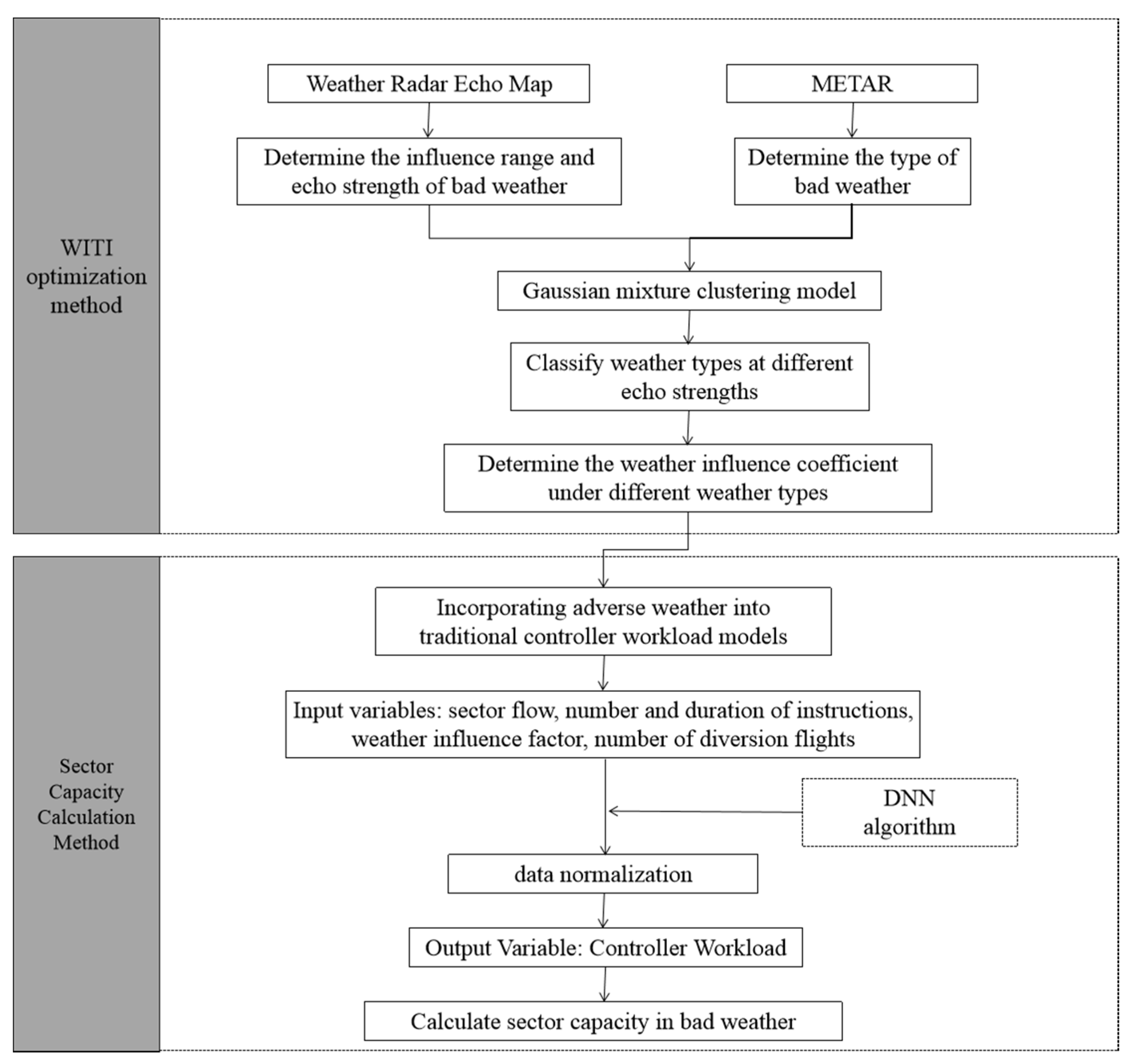
The weather-influence coefficient in the WITI model was optimized mainly by refining the bad-weather types, and the severity of weather was expressed in the form of echo intensity. However, there was no suitable measurement relationship between echo intensity and bad-weather types to classify them. The relationship between the three bad-weather types and radar echo intensities was investigated using a Gaussian mixture clustering model.

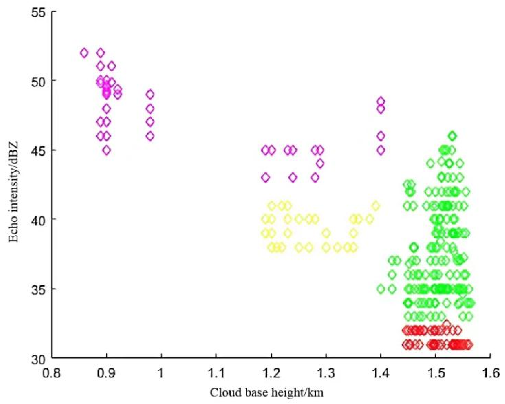
In cloudy weather, the severity of weather can be expressed by the cloud base height, and so the clustering model used two indexes (cloud base height and echo intensity) in the clustering analysis; the results are shown in Figure 5.

According to the clustering results, rainy weather could be divided into four types: high-cloud-base echo intensity, high-cloud-base echo intensity, middle-cloud-base echo intensity, and low-cloud base echo intensity; these types of weather accounted for 21.76%, 53.98%, 13.67%, and 9.59% of cases, respectively.

The visibility can be used to indicate the severity of sand-dust weather, and so the clustering model used two indicators (visibility and echo intensity) in the clustering analysis; the results are shown in Figure 6.

According to the clustering results, dust weather could be divided into five types: high visibility and low echo intensity, high visibility and moderate echo intensity, moderate visibility and moderate echo intensity, moderate visibility and high echo intensity, and low visibility and high echo intensity; these types of weather accounted for 7.32%, 37.62%, 33.45%, 12.60%, and 9.01% of cases, respectively.

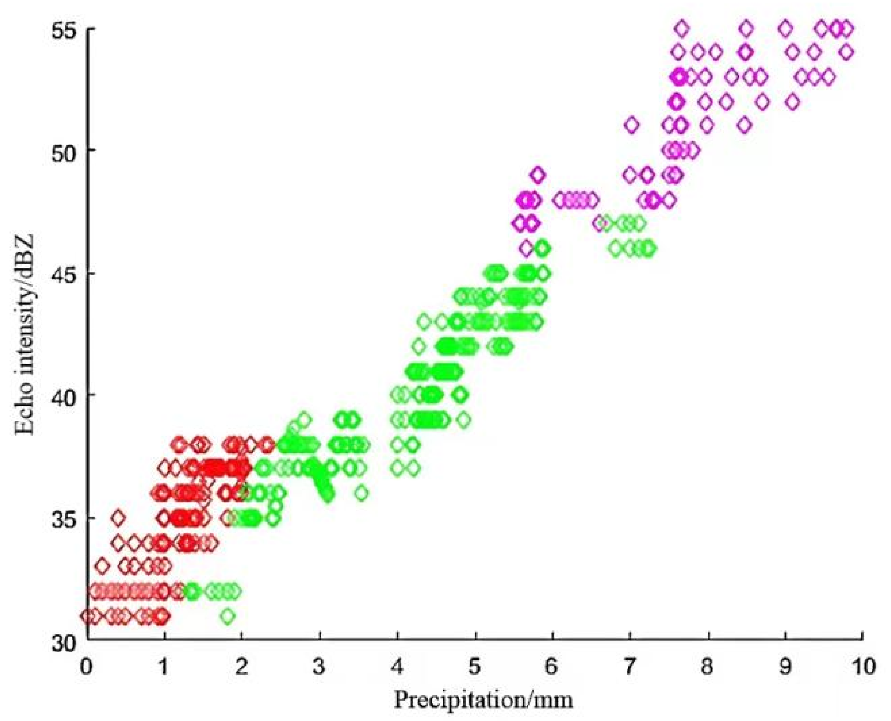
The severity of bad weather can be expressed by the precipitation in heavy-precipitation weather, and so the clustering analysis was performed using precipitation and echo intensity; the results are shown in Figure 7.

According to the clustering results, heavy-precipitation weather could be divided into three types: low precipitation and low echo intensity, moderate precipitation and moderate echo intensity, and high precipitation and high echo intensity; these types of weather with low precipitation and echo intensity accounted for 29.72%, 49.67%, and 20.61% of cases, respectively.

Therefore, bad weather could be divided into high cloud base and low echo intensity, high cloud base and low–high echo intensity, middle cloud base and high echo intensity, low cloud base and high echo intensity, high visibility and low echo intensity, moderate visibility and echo intensity, moderate visibility and high echo intensity, low visibility and high echo intensity, and low precipitation and low echo intensity. There were 12 types of bad weather with high precipitation and high echo intensity, for which the weather-influence coefficient could be obtained by calculating the ratio of the numbers of affected flights to planned flights, as listed in

Table 2. Weather-influence coefficients for various types of bad weather.

Type of Bad Weather (a)	Specific Meaning	Weather-Influence Coefficient $({\mathit{W}}_{\mathit{a}})$
1	High echo intensity and high cloud base (including cloudy weather)	0.19
2	High cloud base and low–high echo intensity (including cloudy weather)	0.27
3	High echo intensity and middle cloud base (including cloudy weather)	0.39
4	Low cloud base and high echo intensity (including cloudy weather)	0.51
5	High visibility and low echo intensity (including high blowing and floating dust weather)	0.21
6	Echo intensity in high visibility (including high blowing and floating dust weather)	0.32
7	Echo intensity in moderate visibility (including high blowing and floating dust weather)	0.41
8	Moderate visibility and high echo intensity (including high blowing and floating dust weather)	0.48
9	Low visibility and high echo intensity (including high blowing and floating dust weather)	0.59
10	Low precipitation and low echo intensity (including thunderstorms)	0.57
11	Echo intensity in moderate precipitation (including thunderstorms)	0.72
12	High precipitation and high echo intensity (including thunderstorms)	1

.

Our approach for optimizing the weather-influence coefficient in the WITI model has overcome the deficiency of only being able to express the influence of thunderstorm weather on aircraft flights. The severity of bad weather has been graded and quantified according to the echo intensity, and so that the weather-influence coefficient can more accurately and clearly reflect the type and influence of the severity of bad weather in the study area.

4.2.2. Determination of the Number of Diverted Flights

The types of bad weather classified using a fuzzy mathematics calculation method are presented in

Table 3. Classification of severe-weather grades.

Bad Weather Rating	Types of Bad Weather
1	11, 12
2	4, 8, 9, 10
3	1, 2, 3, 5, 6, 7

.

The route directions of routes are expressed by waypoints at critical points in each sector. The relationship between the routes and the waypoints at Yinchuan Hedong International Airport is presented in

Table 4. Route classification.

Route Path Number	Path
R1	Exit in the direction of OPULI
R2	Exit in the direction of DOXED
R3	Exit in the direction of DOMVA
R4	Exit in BELIP direction
R5	Go in the direction of OPULI
R6	Advance in the direction of AGVEN
R7	Heading in the direction of IDGOB
R8	LUVKO heading in

.

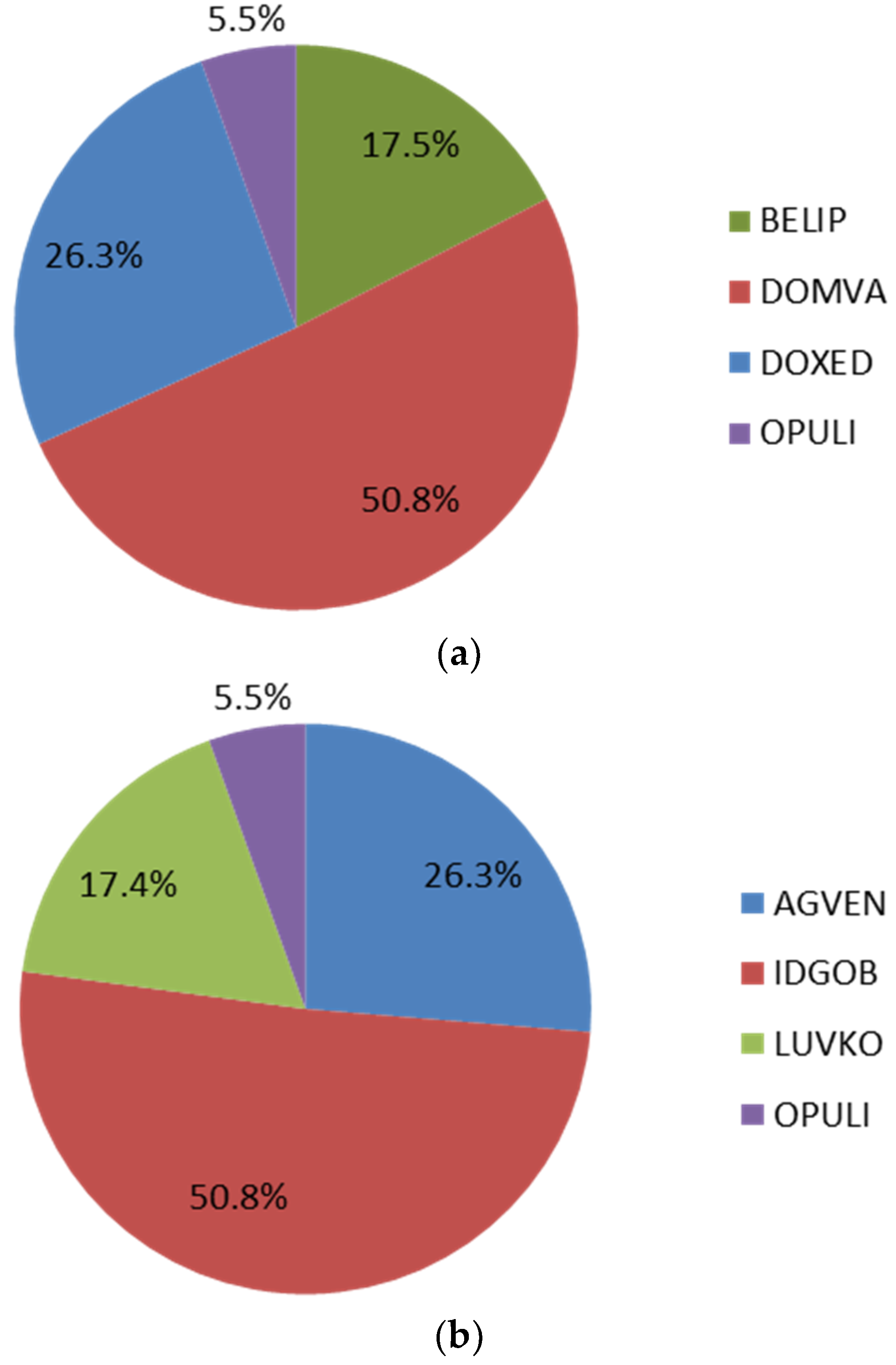
The data for 2019 were imported into the AIRTOP software model on a daily basis for the simulations. The air traffic flow in each route was determined, as was the flow distribution ratio according to the flow passing through the inbound and outbound waypoints. The statistical results are shown in Figure 8.

According to the statistical results, the inbound and outbound flights of Yinchuan Hedong International Airport accounted for 51.21% and 48.79% of the total flights, respectively. The flow distribution ratio on each route could be obtained by combining the inbound and outbound flow distribution for each route waypoint. The specific distribution is presented in

Table 5. Statistics of the proportion of route traffic in each route.

Route Path Number	Path	Proportion of Route Traffic
R1	Exit in the direction of OPULI	2.70%
R2	Exit in the direction of DOXED	13.11%
R3	Exit in the direction of DOMVA	24.80%
R4	Exit in BELIP direction	8.75%
R5	Go in the direction of OPULI	2.80%
R6	Advance in the direction of AGVEN	13.16%
R7	Heading in the direction of IDGOB	26.00%
R8	LUVKO heading in	8.68%

.

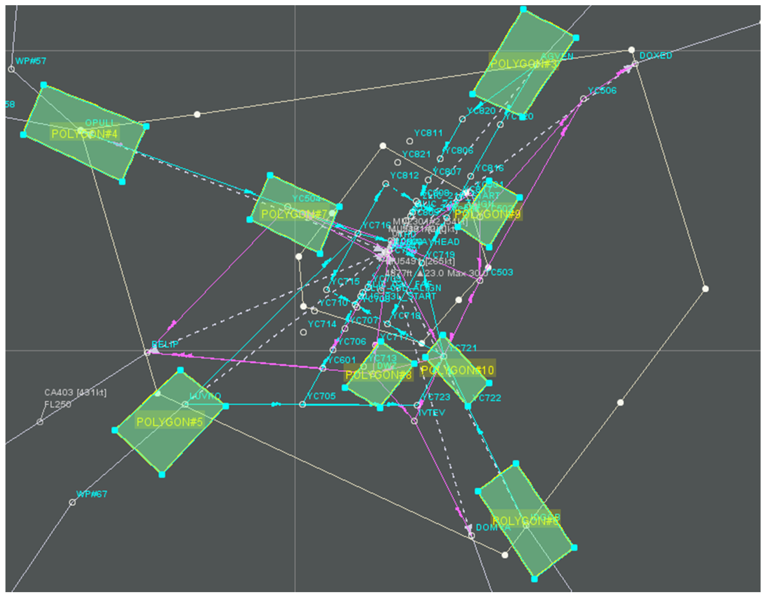
According to the position of the boundary points for the approach and departure routes, the flight-restricted area of each route was determined in the AIRTOP model. Simulations were performed based on the annual takeoff and landing operations at Yinchuan Hedong International Airport in 2019, and different restricted areas were designed according to the flow direction of the inbound and outbound routes. The specific design details are shown in Figure 9.

The opening hours of restricted areas are set according to when bad weather occurs, and the blocking degree of restricted areas is defined according to the route-availability values. The flight arrivals and departures in 2019 were simulated according to the route-availability values calculated under different grades of bad weather. When the restricted areas are opened and run according to the system settings, the aircraft in the system that is scheduled to fly over the restricted areas will be intercepted, and the intercepted aircraft will be those that need to be diverted due to bad weather.

After using the data to train the simulation system, the number of diverted flights on different routes in different bad-weather grades could be obtained. The specific results are listed in

Table 6. Numbers of flights affected by bad weather on each route.

Path Number	Grade of Bad Weather
	1	2	3
R1	6	3	2
R2	31	15	8
R3	59	29	14
R4	21	10	6
R5	7	4	3
R6	32	16	7
R7	62	31	16
R8	20	11	6

.

4.2.3. Calculation of Sector Capacity in Bad Weather

The main research data utilized were 20,460 data points extracted from the call records of controllers in bad weather during mid-2019. The data for 24 June were selected as sample data, and data for another 10 days were used in the model as training data. Yinchuan Hedong International Airport is divided into two sectors: inner sector and outer sector. The operation modes of these two sectors were implemented with a time update unit of 1 h. The results are shown for sample data on 24 June as an example.

Sector flow (S), instruction times (N), instruction duration (I), and optimized weather-influence coefficient (W) were calculated by Gaussian mixture clustering, and the number of diverted flights (C) was calculated using the route-availability model. The training form was the DNN algorithm, and the time update unit was 1 h.

Before the experiments, we compared the DNN algorithm with the Hybrid Kernel SVM algorithm. We selected three groups of 360 pieces of data as test samples, and each group of data is equipped with the evaluation criteria of air traffic control experts. Both methods only take instruction times (N) and instruction duration (I) as input variables, and the output is the controller workload.

In the Hybrid Kernel SVM Algorithm, we choose the convex combination form of the Gaussian kernel function and polynomial kernel function as the hybrid kernel function, which can theoretically improve the generalization ability and learning ability, and has the characteristics of two basic kernel functions at the same time. The hybrid kernel function is constructed as follows:

$$k(x,x^{\prime })=m{k}_{poly}(x,x^{\prime })+(1-m)k_{rbf}(x,x^{\prime })$$

(15)

There are 4 parameters to be considered in the proposed hybrid kernel function: the order $d$ of the polynomial kernel function, the kernel width $s$ of the RBF kernel, the weight coefficient $m$ and the penalty coefficient $C$. The final parameter optimization results are as follows in

Table 7. Parameter value result.

Parameter	Value
the penalty parameter $C$	24
the RBF kernel parameter $s$	2–8
the order parameter $d$	3
the weight coefficient parameter $m$	0.57

.

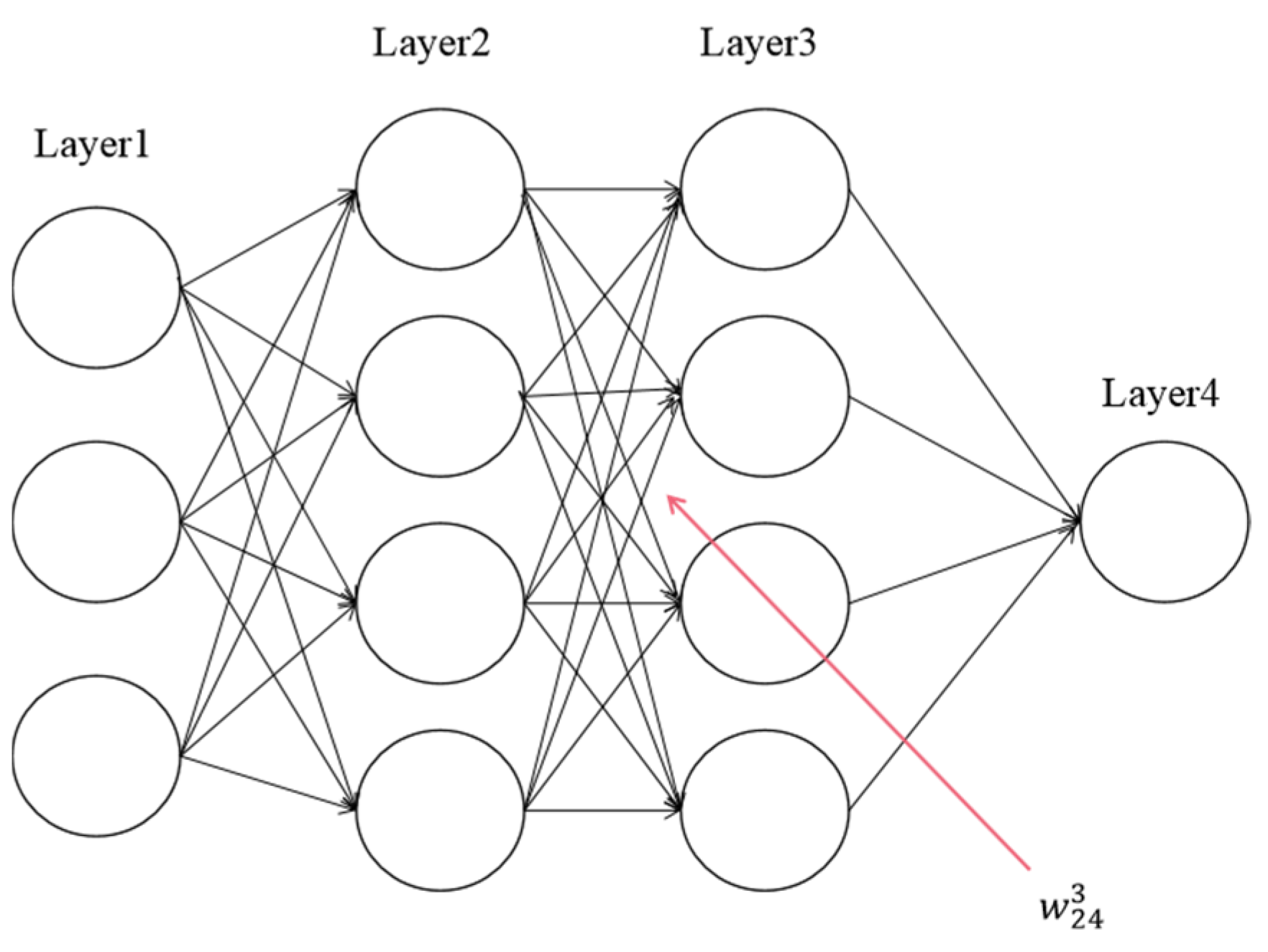
In the DNN algorithm, according to the relationship between the input variable and the output variable and the requirement of the target value of the model error, the number of layers of the hidden layer is determined to be 2. The number of nodes in each layer is determined by the formula in the range of [2,3,4,5], and the size of the evaluation mean square error value in each case is obtained according to the calculation. When the number of hidden layers is 2 and the number of nodes is 3 and 4, respectively, the mean square error of the system is the smallest 0.2267. Therefore, the model structure of the DNN algorithm is 2-{3-4}-1. According to the comparison with the expert evaluation criteria, the results of both methods are as follows in

Table 8. Validation results obtained by two methods.

Method	Validation Results
DNN algorithm	0.92529
Hybrid Kernel SVM algorithm	0.91835

.

It can be seen that the accuracy of the two methods is similar in this type of application. Considering that in the follow-up experiments, the number of variables will increase. The DNN algorithm can provide a good research model for studying the nonlinear relationship between multiple variables, and it’s error correction of it can be used to obtain a more accurate result. Therefore, we choose to use the DNN algorithm in this paper. Ten groups of 1200 pieces of data with input variables were trained using the DNN forward-propagation algorithm. The input variables of each group were divided into sector flow, talk time of controllers per hour, talk times, diverted trips, and optimized weather-influence coefficients. There were 120 pieces of input sample data in each group. The workload of output variable controllers was calculated, and the output sample data are presented in

Table 9. Controller workload after model training.

Time Interval	Controller Workload	Time Interval	Controller Workload
00:00–01:00	626.73	12:00–13:00	2030.94
01:00–02:00	142.99	13:00–14:00	1801.13
02:00–03:00	0	14:00–15:00	1002.32
03:00–04:00	0	15:00–16:00	1465.82
04:00–05:00	0	16:00–17:00	1332.77
05:00–06:00	0	17:00–18:00	1237.27
06:00–07:00	0	18:00–19:00	1576.34
07:00–08:00	932.00	19:00–20:00	2385.04
08:00–09:00	1465.82	20:00–21:00	1576.34
09:00–10:00	1688.11	21:00–22:00	1321.13
10:00–11:00	1702.43	22:00–23:00	1302.36
11:00–12:00	1576.34	23:00–24:00	1002.29

.

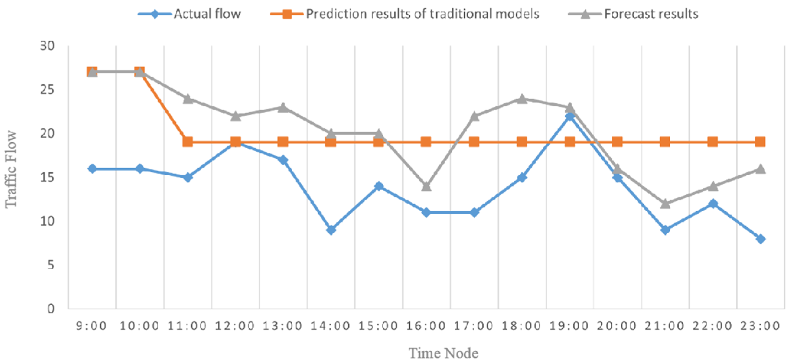
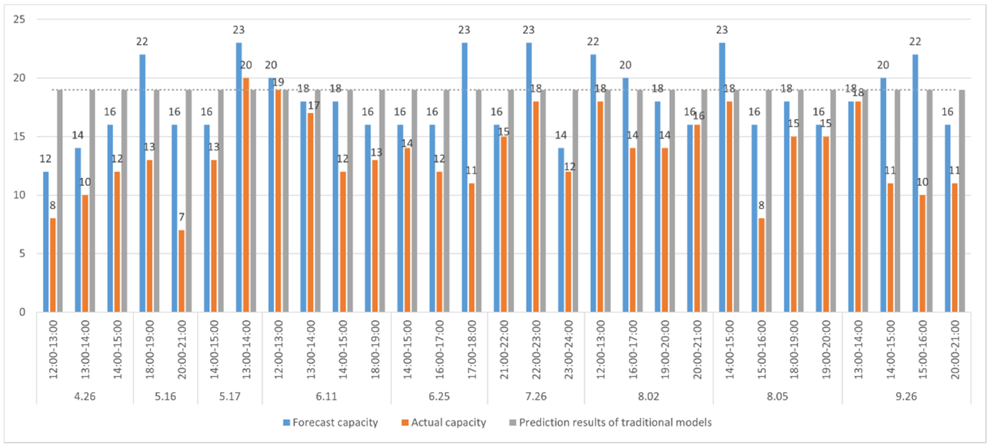
The model calculations have revealed the workload of controllers in the sector of Yinchuan Hedong International Airport under the influence of bad weather on 24 June 2019. Regression analysis was carried out between controller workload and the number of aircraft during this period, and the functional relationship between them was determined. The corresponding sector capacity during this period was calculated by the workload of controllers obtained in the model training. The calculation results are presented in

Table 10. Sector capacities predicted by the model.

Time Interval	Sector Capacity/Route	Time Interval	Sector Capacity/Route
00:00–01:00	12	12:00–13:00	22
01:00–02:00	16	13:00–14:00	23
02:00–03:00	20	14:00–15:00	20
03:00–04:00	23	15:00–16:00	20
04:00–05:00	26	16:00–17:00	14
05:00–06:00	27	17:00–18:00	22
06:00–07:00	27	18:00–19:00	24
07:00–08:00	26	19:00–20:00	23
08:00–09:00	26	20:00–21:00	16
09:00–10:00	27	21:00–22:00	12
10:00–11:00	27	22:00–23:00	14
11:00–12:00	24	23:00–24:00	16

.

4.3. Analysis

The capacity prediction results in Table 8 for the traditional WITI model and the actual traffic verify the feasibility of the present research model. The results are compared in Figure 10.

The time node of the comparison curve was selected from 09:00 to 23:00 on 24 June, during which six types of bad weather appeared. This began at 11:00, after which the sector capacity began to change accordingly; there was no influence of bad weather in the sector from 09:00 to 11:00. The predicted results for the traditional WITI model were consistent with the actual observations, and the sector capacity was 27 operations/hour. At 11:00 the sector capacity predicted by WITI model changed to 19 operations/hour and then remained constant. Meanwhile, the predicted results for the DNN model varied from 12 to 27 operations/hour according to different sector capacities of severe-weather types. In order to further compare the prediction fit of the sector capacity between the traditional prediction model and the DNN model, representative time segments were selected from the database for data comparisons; the results are shown in Figure 11.

It can be seen from Figure 11 that when bad weather occurred, the forecasting capacity of the traditional forecasting model was 19 operations/hour, and this did not change with different types of bad weather. The forecasts of the DNN model varied from 12 to 23 operations/hour according to different types of bad weather. This is because, in the traditional WITI model, the weather-influence coefficient only has a value of 1 or 0; that is, it can only identify whether or not there is bad weather in the sector, without quantifying its severity. The prediction result for the sector capacity was 19 operations/hour when bad weather was present and 27 operations/hour when it was not present. The DNN model adds the optimized weather-influence coefficient to predict the sector capacity under corresponding conditions according to different types of bad weather, which makes the prediction result closer to the actual operating situation.

By sorting and analyzing the training data, the sector capacity prediction results under different types of bad weather could be obtained; the results are presented in

Table 11. Sector capacities under different types of bad weather.

Type of Bad Weather (a)	Specific Meaning	Sector Capacity (Operations/Hour)
0	Normal weather	27
1	High echo intensity and high cloud base (including cloudy weather)	22
2	High cloud base and low–high echo intensity (including cloudy weather)	23
3	High echo intensity and middle cloud base (including cloudy weather)	20
4	Low cloud base and high echo intensity (including cloudy weather)	18
5	High visibility and low echo intensity (including high blowing and floating dust weather)	24
6	Echo intensity in high visibility (including high blowing and floating dust weather)	22
7	Echo intensity in moderate visibility (including high blowing and floating dust weather)	23
8	Moderate visibility and high echo intensity (including high blowing and floating dust weather)	23
9	Low visibility and high echo intensity (including high blowing and floating dust weather)	16
10	Low precipitation and low echo intensity (including thunderstorms)	16
11	Echo intensity in moderate precipitation (including thunderstorms)	14
12	High precipitation and high echo intensity (including thunderstorms and thunderstorms)	12

.

The input variables of the model are the sector flow, instruction times, instruction duration, optimized weather-influence coefficient, and the number of diverted flights, and the output variable is the controller workload. The first three input variables are basic variables for calculating controller workload, while the weather-influence coefficient reflects the actual sector capacity affected by weather during the specific time period, and the number of diverted flights reflects that controllers need to issue instructions to coordinate aircraft conflicts during this time period.

After model training, the controller workload involves predicting the sector capacity for the day, and at the same time, the traditional controller model is used to predict the sector capacity of the day. Comparing the two groups of data with the actual sector values revealed that the results predicted by the controller workload model considering the influence of bad weather were more consistent with the actual situation.

5. Conclusions

This study analyzed a sector capacity model based on an improved WITI index under the influence of bad weather with the aim of identifying the sector capacity for different types of bad weather. Weather-radar echo charts and the controller’s call records were taken as the research objects, and the WITI model was optimized by extracting weather information data from these charts, so that it can quantify the adverse effects of different types of bad weather. By combining a route-availability model and AIRTOP software modeling, the aircraft operations that need to be diverted under bad weather conditions were obtained through simulations. Finally, the DNN algorithm was used to calculate the influence of bad weather and the number of diverted flights, so as to obtain the controller workload in the presence of bad weather, and the sector capacity was calculated according to the controller workload model.

This research paper has described a theoretical model for calculating the sector capacity in bad weather. Most importantly, the model can be used to evaluate the sector capacity more accurately for different types of bad weather. Providing data support for making flight plans in bad weather will help to improve the punctuality rate of flights and travel efficiency.

At present, this paper studies the capacity of a single airport within a sector, and the research on severe weather currently focuses on thunderstorms and floating dust. In future work, we will consider airports with different levels of busyness in different geographical locations, such as Shanghai Hongqiao International Airport and Chengdu Shuangliu International Airport, and explore the impact of different bad weather types on sector capacity.

References

1. Civil Aviation Administration of China. Statistical Bulletin on the Development of Civil Aviation Industry in 2019; Civil Aviation Administration of China: Beijing, China, 2020.
2. McCrea, M.V.; Sherali, H.D.; Trani, A.A. A probabilistic framework for weatherbased rerouting and delay estimations within an Airspace Planning model. Transp. Res. Part C Emerg. Technol. 2008, 16, 410–431. [Google Scholar] [CrossRef]
3. Bailey, R. Human Performance Engineering: Designing High Quality, Professional User Interfaces for Computer Products Applications and Systems, 3rd ed.; Prentice Hall: Hoboken, NJ, USA, 1996. [Google Scholar]
4. Janic, M.; Tosic, V. Terminal Airspace Capacity Model. Transp. Res. Part A 1982, 16, 253–260. [Google Scholar] [CrossRef]
5. Janic, M. Enroute sector capacity model. Transp. Sci. 1991, 25, 215–224. [Google Scholar] [CrossRef]
6. Tofukuji, N. An Enroute ATC Simulation Experiment for Sector Capacity Estimation. IEEE Trans. Control Syst. Technol. 1993, 1, 138–143. [Google Scholar] [CrossRef]
7. Tofukuji, N. An Airspace Design and Evaluation of En-route Sector by Air Traffic control Simulation Experiments. Electron. Commun. Jpn. Part 1 (Commun.) 1996, 79, 103–113. [Google Scholar] [CrossRef]
8. Chatterji, G.B.; Sridhar, B. Neural Network Based Air Traffic Controller Workload Prediction. In Proceedings of the American Control Conference, San Diego, CA, USA, 2–4 June 1999; pp. 2620–2624. [Google Scholar]
9. Basu, A.; Mitchell, J.S.B.; Sabhnani, G. Geometric algorithms for optimal airspace design and air traffic controller workload balancing. In Proceedings of the 9th Workshop on Algorithm Engineering and Experiments (ALENEX), San Francisco, CA, USA, 6 January 2007. [Google Scholar]
10. Wang, B. Research on Controller Workload Evaluation Based on Air Traffic Complexity. Master’s Thesis, Nanjing University of Aeronautics and Astronautics, Nanjing, China, 2008. [Google Scholar]
11. Yang, S. Research on Capacity Evaluation Technology of Multi-Sector Coupling Operation. Master’s Thesis, Nanjing University of Aeronautics and Astronautics, Nanjing, China, 2015. [Google Scholar]
12. Li, S. Research on Capacity Evaluation Method under Sector Coupling Conditions. In Proceedings of the 1st Annual Conference on Air Traffic Management System Technology, Chinese Society of Command and Control, Nanjing, China, 29 November 2018; Volume 4, pp. 149–152. [Google Scholar]
13. DeLaura, R.A. Evaluation of Consolidated Storm Prediction for Aviation (CoSPA) 0–8 Hour Convective Weather Forecast Using the Airspace Flow Program Blockage-based Capacity Forecast (“The Matrix”); Project ReportATC-385; MIT: Cambridge, MA, USA, 2011. [Google Scholar]
14. Chen, J.; Chen, L.; Sun, D. Air traffic flow management under uncertainty using chance-constrained optimization. Transp. Res. Part B Methodol. 2017, 102, 124–141. [Google Scholar] [CrossRef]
15. Liu, J.; Zhu, X.; Wu, Y.; Yin, W.; Zeng, X. Sector capacity evaluation considering the workload of WITI and controllers. Aviat. Comput. Technol. 2018, 48, 11–14+19. [Google Scholar]
16. Zhang, W.; Wang, Y.; Yan, W.; Li, C. Multi-sector dynamic capacity evaluation method under severe weather. Firepower Command Control 2019, 44, 126–130+140. [Google Scholar]
17. Michalek, D.; Balakrishnan, H. Dynamic reconfiguration of terminal airspace during convective weather. In Proceedings of the 2010 49th IEEE Conference on Decision and Control, CDC 2010, Atlanta, GA, USA, 15–17 December 2010; pp. 4875–4881. [Google Scholar]
18. Welch, J.D.; Andrews, J.W.; Martin, B.D. Macroscopic Workload Model for Estimating EN Route Sector Capacity; NASA Ames Research Center: Mofferr Field, CA, USA, 2011.
19. Agustin, A.; Alonso-Ayuso, A.; Escudero, L.F.; Pizarro, C. On air traffic flow management with rerouting. Part II: Stochastic case. Eur. J. Oper. Res. 2012, 219, 167–177. [Google Scholar] [CrossRef]
20. Bengio, Y. Learning Deep Architectures for AI. Found. Trends® Mach. Learn. 2009, 2, 1–127. [Google Scholar] [CrossRef]
21. Mi, C.; Shao, C.; He, H.; He, C.; Ma, H. Evaluating Tissue Mechanical Properties Using Quantitative Mueller Matrix Polarimetry and Neural Network. Appl. Sci. 2022, 12, 9774. [Google Scholar] [CrossRef]
Figure 1. The architecture diagram of the overall system.
Applsci 12 10114 g001
Figure 2. 4 layers DNN structure.
Applsci 12 10114 g002
Figure 3. Flow chart of model building.
Applsci 12 10114 g003
Figure 4. DNN model structure.
Applsci 12 10114 g004
Figure 5. Clustering results for rainy weather.
Applsci 12 10114 g005
Figure 6. Schematic diagram of dust weather clustering results.
Applsci 12 10114 g006
Figure 7. Schematic diagram of clustering results for heavy-precipitation weather.
Applsci 12 10114 g007
Figure 8. Flow distribution for approach and departure. (a) Departure flow distribution, (b) Approach flow distribution.
Applsci 12 10114 g008
Figure 9. Schematic diagram of flight-restricted areas of the approach and departure routes.
Applsci 12 10114 g009
Figure 10. Comparison of typical daily data.
Applsci 12 10114 g010
Figure 11. Comparison of data over multiple days.
Applsci 12 10114 g011