A Semi-Supervised Extreme Learning Machine Algorithm Based on the New Weighted Kernel for Machine Smell

Abstract

At present, machine sense of smell has shown its important role and advantages in many scenarios. The development of machine sense of smell is inseparable from the support of corresponding data and algorithms. However, the process of olfactory data collection is relatively cumbersome, and it is more difficult to collect labeled data. However, in many scenarios, to use a small amount of labeled data to train a good-performing classifier, it is not feasible to rely only on supervised learning algorithms, but semi-supervised learning algorithms can better cope with only a small amount of labeled data and a large amount of unlabeled data. This study combines the new weighted kernel with SKELM and proposes a semi-supervised extreme learning machine algorithm based on the weighted kernel, SELMWK. The experimental results show that the proposed SELMWK algorithm has good classification performance and can solve the semi-supervised gas classification task of the same domain data well on the used dataset.

1. Introduction

At present, machine smell has been applied in many fields. Many people try to use machine smell to solve related problems. For example, Xu et al. used an electronic nose system to evaluate the quality of tea leaves based on the volatile components of tea leaves and tea infusions, demonstrating the feasibility of the electronic nose system in qualitative and quantitative analysis of tea quality [1]. With the development of sensor technology, signal processing technology and machine learning technology [2,3,4], various solutions have emerged in the field of machine smell technology. Liu et al. used four machine learning methods to classify wine, concluding that BP neural network has a better recognition effect [5]. In environmental detection, Zhang et al. [6]. proposed a new neural network method based on a chaos optimization algorithm and combined it with a portable electronic nose to estimate the indoor pollutant concentration. It has been verified that this method is superior and efficient. In the medical field [7,8,9,10], the development of sensor technology and the neural network has also promoted the development of machine sense of smell. VA B et al. used a robotic olfactory system based on a MOS sensor array to analyze breath for non-invasive detection of COPD and lung cancer [11]. Hendrick H et al. proposed a method for non-invasive detection of pulmonary tuberculosis, which analyzed the exhaled breath of tuberculosis patients and ordinary people through an olfactory machine system. They used multiple machine learning methods to classify them [12].

Semi-supervised learning (SSL) is a key problem in the field of pattern recognition and machine learning. It is a learning method combining supervised learning with unsupervised learning. Semi-supervised learning uses a large number of unlabeled data and uses labeled data at the same time to carry out pattern recognition. The basic idea of semi-supervised learning is to use model assumptions in data distribution to build a learner to label unlabeled samples.

Semi-supervised learning aims to discover more data feature information from a small amount of labeled data and a large amount of unlabeled data [13]. The idea of semi-supervised learning has been used in various applications, such as a semi-supervised learning workflow based on a generative adversarial network (GAN) for acoustic impedance inversion [14], deep transfer learning for few-shot SAR image classification [15], a SAR target detection network based on a semi-supervised learning and attention mechanism [16] and Semi-supervised few-shot learning [17]. Commonly used methods for semi-supervised learning include self-training, co-training, transductive support vector machines and graph-based methods.

In this study, the semi-supervised classification problem of the same domain data in the field of machine smell is studied at the algorithm level. The so-called same-domain data refers to the data collected successively when the sensor does not have drift or has a slight drift problem, usually collected under the same conditions using the same equipment for a continuous period. This paper proposes a semi-supervised extreme learning machine algorithm based on the weighted kernel (SELMWK). Aiming at the problem that machine olfactory experiments are usually cumbersome and it is relatively difficult to collect labeled data, the semi-supervised classification problem of the same domain data is caused. Inspired by a Semi-supervised Extreme Learning Machine (SSELM) and multi-core learning, the SELMWK algorithm is proposed. It improves the poor operation stability of semi-supervised extreme learning machines due to random hidden layers, and avoids the poor applicability of single-core learning. The effectiveness of the algorithm is verified from two data sets. It has been verified that this algorithm is better than the proposed SSELM and Semi-supervised Extreme Learning Machine (SKELM) algorithms.

2. Related Work

The self-training algorithm was originally proposed by Yarowsky, who used this algorithm for semantic elimination to predict the meaning of words based on context [18]. In [19], Li et al. proposed a self-learning semi-supervised deep learning network for identifying fake news on the network. By adding a belief network layer, the accuracy of the network was improved.

The co-training algorithm was first proposed by A.Blum and T.Mitchell in [20] for the task of web page classification. Yaslan and Cataltepe proposed a random subspace collaborative algorithm, which uses the random subspace generated by the algorithm to perform semi-supervised ensemble learning on unlabeled data. Experiments show that the algorithm achieves good results on real data sets [21]. In 2018, Qiao et al., inspired by the collaborative training method, proposed a deep collaborative training algorithm to complete the task of semi-supervised image recognition by training multiple neural networks into multiple different views. Demonstrated better performance on the dataset [22].

Joachims T. used transduction support vector machines for the task of text classification with great results [23]. In the literature [24], N. Zemmal et al. proposed a semi-supervised support vector machine algorithm for breast cancer classification. First, three types of features were extracted, and the dimension of the feature vector was reduced by using a genetic algorithm. Finally, the semi-supervised classification was carried out. Classifier S3VM.

The graph semi-supervised method mainly uses labeled and unlabeled data to construct a data graph and propagates the labels according to the adjacency relationship. Combining the knowledge of graph Laplacian and multi-feature learning, Zhang et al. proposed a semi-supervised joint learning model based on multi-feature kernels to improve the robustness of electronic noses [25].

3. Dataset

3.1. Dataset Description

In this study, two public datasets were selected to verify the effect of the SELMWK algorithm, namely:

(1)

Dataset 1: The gas delivery platform facility at the Chemical Signaling Laboratory of the Institute of Biological Circuits, University of California, San Diego, was selected using sensors from A Vergara et al. and published this dataset on the UCI Machine Learning Repository [26,27]. The dataset has a total of 13,910 measurements, using a sensor array consisting of 16 gas sensors to collect data for 6 different gases at different concentrations. The measurement system platform provides the versatility to obtain the concentration of desired chemicals with high accuracy and reproducibility, thereby minimizing common errors caused by human intervention and allowing focus on chemical sensors. The resulting dataset consists of records from six different pure gaseous substances, with 8 data points selected from each specific sensor as feature points over the entire time series, so a set of data yields a total of 8 × 16 = 128-dimensional feature vectors. The dataset was divided into 10 batches in total, which were collected in different months.

Table 1. Data volume for different sample gases in 10 batches 6.

Batch ID	Month	Acetone	Acetaldehyde	Ethanol	Ethylene	Ammonia	Toluene	Total
Batch 1	1–2	90	98	83	30	70	74	445
Batch 2	3–10	164	334	100	109	532	5	1244
Batch 3	11–13	365	490	216	240	275	0	1586
Batch 4	14, 15	64	43	12	30	12	0	161
Batch 5	16	28	40	20	46	63	0	197
Batch 6	17–20	514	574	110	29	606	467	2300
Batch 7	21	649	662	360	744	630	568	3613
Batch 8	22, 23	30	30	40	33	143	18	294
Batch 9	24, 30	61	55	100	75	78	101	470
Batch10	36	600	600	600	600	600	600	3600

shows the details of dataset 1.

(2)

Dataset 2: Select the gas data collected by J. Fonollosa et al. using 8 MOX sensors [28]. They exposed the sensor arrays to 10 different ethanol, methane, ethylene, and carbon monoxide concentrations. The duration of each experiment is 600 s, and the conductivity of each sensor is 100 Hz, so a set of data has 60,000 × 8 = 480,000 data. In the experiments of this chapter, in order to train a classifier with better applicability and make it better to deal with gases of different concentrations, the same type of gas with different concentrations is set as the same sample, and only the type of target gas is analyzed. For classification prediction, the labels of the same gas samples with different concentrations are set to the same class.

Table 2. Eight MOX Sensors.

Sensor Type	Sensitive Gas
TGS2611 5.65V	Methane, natural gas
TGS2612 5.65V	Methane, propane, butane
TGS2610 5.65V	Propane, butane
TGS2602 5.65V	Toluene and other VOC volatile gases
TGS2611 5.00V	Methane, natural gas
TGS2612 5.00V	Methane, propane, butane
TGS2610 5.00V	Propane, butane
TGS2602 5.00V	Toluene and other VOC volatile gases

is the information of 8 MOX sensors, and

Table 3. Amounts and concentrations of different gases in dataset 2.

Gas Type	Number of Samples	Concentration (ppm)
Ethanol	160	12.5, 25, 37.5, 50, 62.5, 75, 87.5, 100, 112.5, 125
Methane	160	25, 50, 75, 100, 125, 150, 175, 200, 225, 250
Vinyl	160	12.5, 25, 37.5, 50, 62.5, 75, 87.5, 100, 112.5, 125
Carbon Monoxide	160	25, 50, 75, 100, 125, 150, 175, 200, 225, 250

is the number of samples and concentrations of different gases in this data set.

(3)

It can be known from Table 2 and Table 3 that the 8 MOX sensors have good sensitivity to the four gases to be measured so that the response curve of the sensor can be avoided because the gas to be measured does not react with the sensor array. The lack of more useful information will eventually make the gas classification effect less effective. At the same time, it can be seen from the number of samples that the number of four samples is relatively uniform so that the data skew problem will not be caused due to the excessive amount of data of certain sample gas, thereby reducing the accuracy of gas classification.

3.2. Dataset Processing

Data Cropping and Filtering

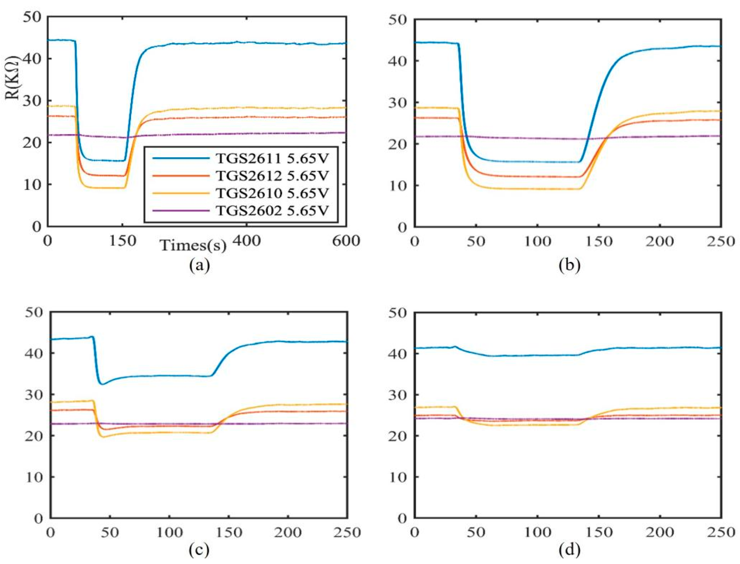
Different from the data in Dataset 1, Dataset 2 provides the complete data within 600 s without preprocessing and data extraction. This means that if the data in this dataset is used directly, each sample will reach a dimension of 480,000. Figure 1 is the response curve of different gas sensors:

Figure 1a is a graph of the sensor response for raw 250 ppm methane gas. It can be seen from the figure that the resistance value of the sensor is not always changing. Only during the desorption process and a short period during the reaction process does the resistance value of the sensor change due to the redox reaction. When in the stable and maximum response stages, the resistance value basically does not change or fluctuates little. Therefore, there is too much redundant information in the 480,000-dimensional data. Excessive data dimensions will not only greatly increase the computational complexity of model training but also cause model training to be slow. Therefore, it is necessary to perform dimensionality reduction operations on the data. In addition, when processing the data in the data set, it is found that due to data preservation reasons, many data samples in the public data set do not reach the dimension of 480,000, and there is data loss, which will bring difficulties to the subsequent feature extraction. In order to ensure the uniformity of the dimensions of the sample data, the entire data set is screened and the data samples are trimmed. First, discard the samples with too much missing data, and reduce the entire data set to 600 data samples. After that, the data is trimmed to reduce the amount of data in the two cleaning processes and the stabilization stage, and finally, the dimension of each sample is reduced to 25,000 × 8 = 200,000.

Figure 1b–d shows the data response curves of trimmed 250 ppm methane gas, 25 ppm methane gas and 250 ppm carbon monoxide, respectively. By comparing Figure 1b,c, it can be seen that the sensor response curves of two gases with different concentrations but the same type in the same sensor array are different. It can be seen that the gas with higher concentration makes the resistance value of the sensor change more, but the changing trend of the resistance value of each sensor is roughly the same. However, it can be seen in Figure 1b,d that the response values and changing trends of the sensor arrays are different at the same concentration of carbon monoxide gas and methane gas. The pattern recognition algorithm of machine smell is to classify the gas by extracting the features in the response curve.

Table 4. Number of different gas samples.

Gas Type	Number of Samples
Ethanol	150
Methane	146
Vinyl	154
Carbon Monoxide	150

below shows the number of different gas samples after cropping the dataset.

4. Method

4.1. Manifold Regularization

Manifold regularization is a graph-based semi-supervised learning method that constructs an undirected graph from labeled and unlabeled data. The vertices of the graph are data samples, and the edges are the similarities between data samples to correlate labeled data with unlabeled data. Since the manifold regularization framework must satisfy the manifold assumption, the smoothness assumption is enforced on the data by minimizing the loss function, which leads to Equation (1):

$${\mathrm{L}}_{\mathrm{m}}=\frac{1}{2}{\displaystyle \sum }_{\mathrm{i},\mathrm{j}}{\mathrm{w}}_{\mathrm{i},\mathrm{j}}{\Vert P\left(y|x_i\right)-P\left(y|x_j\right)\Vert }^2$$

(1)

where ${\mathrm{w}}_{\mathrm{i},\mathrm{j}}$ is the similarity $\mathrm{i}$ between ${\mathrm{x}}_{\mathrm{i}}$ and ${\mathrm{x}}_{\mathrm{j}}$ data, $\mathrm{j}=1,2,\cdots \mathrm{l}+\mathrm{u}$, $\mathrm{l}$ is labeled data, $\mathrm{u}$ is unlabeled data. $\mathrm{P}\left({\mathrm{y}|\mathrm{x}}_{\mathrm{i}}\right)$ and $\mathrm{P}({\mathrm{y}|\mathrm{x}}_{\mathrm{j}})$ are conditional probabilities.

Since the conditional probability calculation is relatively difficult, Equation (1) can be replaced with Equation (2):

$${\tilde{L}}_m=\frac{1}{2}{\displaystyle \sum }_{\mathrm{i},\mathrm{j}}{\mathrm{w}}_{\mathrm{i},\mathrm{j}}{\Vert {\tilde{y}}_i-{\tilde{y}}_j\Vert }^2$$

(2)

where $\widetilde{{\mathrm{y}}_{\mathrm{i}}}$ and $\widetilde{{\mathrm{y}}_{\mathrm{j}}}$ are the prediction results based on the data ${\mathrm{x}}_{\mathrm{i}}$ and ${\mathrm{x}}_{\mathrm{j}}$.

By simplifying Equation (2), Equation (3) can be obtained:

$${\tilde{L}}_m=\mathrm{Tr}\left({\tilde{Y}}^{T}L\tilde{Y}\right)$$

(3)

where $\mathrm{Tr}\left(·\right)$ is the trace of the matrix, $\tilde{\mathrm{Y}} ={[{\tilde{\mathrm{y}}}_1,{\tilde{\mathrm{y}}}_2,\cdots ,{\tilde{\mathrm{y}}}_{\mathrm{l}+\mathrm{u}}]}^{\mathrm{T}}$.

According to the principle of Laplacian, $\mathrm{L}=\mathrm{D}-\mathrm{W}$, $\mathrm{D}$ is a diagonal matrix, and the elements in the matrix are shown in Equation (4):

$${\mathrm{D}}_{\mathrm{ii}}={\displaystyle \sum }_{\mathrm{j}=1}^{\mathrm{l}+\mathrm{u}}{\mathrm{w}}_{\mathrm{i},\mathrm{j}}$$

(4)

W is an adjacency matrix. Set the set of $\mathrm{k}$ nearest neighbors of the data $\mathrm{x}$ to ${\mathrm{N}}_{\mathrm{k}}\left(\mathrm{x}\right)$, then the elements in the adjacency matrix can be obtained by Equation (5):

$${\mathrm{w}}_{\mathrm{i},\mathrm{j}}=\{\begin{array}{c}\exp \left(-\frac{{\Vert x_i-x_j\Vert }^2}{2{\mathsf{\sigma }}^2}\right) {\mathrm{x}}_{\mathrm{i}}\in {\mathrm{N}}_{\mathrm{k}}\left({\mathrm{x}}_{\mathrm{j}}\right) \mathrm{or} {\mathrm{x}}_{\mathrm{j}}\in {\mathrm{N}}_{\mathrm{k}}\left({\mathrm{x}}_{\mathrm{i}}\right)\\ 0 \mathrm{otherwise}\end{array}.$$

(5)

4.2. Semi-Supervised Kernel Extreme Learning Machine Improvement Scheme

The SKELM algorithm has good applicability, but its generalization ability is affected by the kernel function, and the selection of the kernel function often affects the performance of the entire SKELM model. In ordinary SKELM models, only one kernel function is usually used for feature mapping of hidden layers. However, this has drawbacks. For different data, different kernel functions will give the model different performance, so the applicability of a single KELM is not outstanding.

Therefore, to make the trained classifier have a better recognition effect and better stability and generalization ability, this study combines the weighted kernel with the SKELM model and proposes an improved semi-supervised algorithm SELMWK based on the weighted kernel extreme learning machine. The model inherits the advantages of the semi-supervised kernel extreme learning machine and simultaneously makes up for the problem of the insufficient generalization ability of the single-kernel model.

4.2.1. Improved Design of Kernel Function

To increase the applicability of a single kernel function, combining multiple kernel functions is a good solution. In the article [29], Gönen M introduced various ways of combining kernels and showed that using multiple kernels is generally more effective than using a single kernel. After many experiments, the weighted kernel function calculated by this calculation method is applied to this semi-supervised learning task. It also shows a better effect than single-kernel learning. The following is a brief list of four common basic kernel functions:

(1)

Linear Kernel function, whose form is shown in Equation (6):

$$\mathrm{K}\left(x_i,x_j\right)=x_i^T{x}_j$$

(6)

(2)

Polynomial Kernel function,$\mathrm{c}, \mathrm{d}$ are hyperparameters whose form is shown in Equation (7):

$$\mathrm{K}\left(x_i,x_j\right)={\left(x_i^T{x}_j+\mathrm{c}\right)}^{\mathrm{d}}$$

(7)

(3)

Radial basis function kernel, $\mathsf{\sigma }$ is a hyperparameter whose form is shown in Equation (8):

$$\mathrm{K}\left(x_i,x_j\right)=\exp \left(-\frac{{\Vert x_i-x_j\Vert }^2}{2{\mathsf{\sigma }}^2}\right)$$

(8)

(4)

Sigmoid kernel function, where $\mathrm{a}, \mathrm{c}$ are hyperparameters, and its form is shown in Equation (9):

$$\mathrm{K}\left(x_i,x_j\right)=\tanh \left(\mathrm{a}{x}_i^T{x}_j+\mathrm{c}\right)$$

(9)

A linear kernel function is a linear map and a special case of the RBF kernel. RBF can not only non-linearly map data to high-dimensional space but also has fewer parameters than the poly kernel function, so it has less complexity. In addition, when the parameter d in the poly kernel function is high, the element value of the kernel matrix tends to be infinitely large or infinitely small, which greatly increases the difficulty of calculation. Sigmoid as the basic core will not conform to Mercer’s theorem. Therefore, in this study, the RBF kernel is selected as the basic kernel function to obtain the weighted kernel function through a weighted combination. The calculation process is as follows:

First, define a weighted nonlinear mapping function $\mathsf{\Phi }\left(\mathrm{x}\right)$, where $\mathsf{\theta }$ is a weighting parameter, ${\mathsf{\Phi }}_1\left(\mathrm{x}\right)$ and ${\mathsf{\Phi }}_2\left(\mathrm{x}\right)$ are two different nonlinear mapping functions, the form is shown in Equation (10):

$$\mathsf{\Phi }\left(x\right)={\mathsf{\theta }\mathsf{\Phi }}_1\left(x\right)+\left(1-\mathsf{\theta }\right){\mathsf{\Phi }}_2\left(x\right)$$

(10)

Then define a kernel function $\mathrm{K}\left({\mathrm{x}}_{\mathrm{i}},{\mathrm{x}}_{\mathrm{j}}\right)=<\mathsf{\Phi }\left({\mathrm{x}}_{\mathrm{i}}\right),\mathsf{\Phi }\left({\mathrm{x}}_{\mathrm{j}}\right)>$, and bring Equation (10) into it to get Equation (11):

$$\mathrm{K}\left(x_i,x_j\right)={\mathsf{\theta }}^2{\mathrm{K}}_1\left(x_i,x_j\right)+{\left(1-\mathsf{\theta }\right)}^2{\mathrm{K}}_2\left(x_i,x_j\right)+2\mathsf{\theta }\left(1-\mathsf{\theta }\right){\mathrm{K}}_{1,2}\left(x_i,x_j\right)$$

(11)

where ${\mathrm{K}}_1\left({\mathrm{x}}_{\mathrm{i}},{\mathrm{x}}_{\mathrm{j}}\right)=<{\mathsf{\Phi }}_1\left({\mathrm{x}}_{\mathrm{i}}\right),{\mathsf{\Phi }}_1\left({\mathrm{x}}_{\mathrm{j}}\right)>$, ${\mathrm{K}}_2\left({\mathrm{x}}_{\mathrm{i}},{\mathrm{x}}_{\mathrm{j}}\right)=<{\mathsf{\Phi }}_2\left({\mathrm{x}}_{\mathrm{i}}\right),{\mathsf{\Phi }}_2\left({\mathrm{x}}_{\mathrm{j}}\right)>$ is a common basic kernel function, ${\mathrm{K}}_{1,2}\left({\mathrm{x}}_{\mathrm{i}},{\mathrm{x}}_{\mathrm{j}}\right)$ is the cross-kernel function.

When RBF is selected as the basic kernel function, their forms can be expressed as Equations (12)–(14):

$${\mathrm{K}}_1\left(x_i,x_j\right)=\exp \left(-\frac{{\Vert x_i-x_j\Vert }^2}{2{{\mathsf{\sigma }}_1}^2}\right)$$

(12)

$${\mathrm{K}}_2\left(x_i,x_j\right)=\exp \left(-\frac{{\Vert x_i-x_j\Vert }^2}{2{{\mathsf{\sigma }}_2}^2}\right)$$

(13)

$${\mathrm{K}}_{1,2}\left(x_i,x_j\right)={\left(\frac{2{\mathsf{\sigma }}_1{\mathsf{\sigma }}_2}{{{\mathsf{\sigma }}_1}^2+{{\mathsf{\sigma }}_2}^2}\right)}^{\frac{\mathrm{N}}{2}}\exp \left(-\frac{{\Vert 2x_i-x_j\Vert }^2}{{{\mathsf{\sigma }}_1}^2+{{\mathsf{\sigma }}_2}^2}\right)$$

(14)

where ${\mathsf{\sigma }}_1$ and ${\mathsf{\sigma }}_2$ are the parameters of the RBF kernel function, and $\mathrm{N}$ is the dimension of the input data $\mathrm{x}$.

The weighted kernel can be obtained by substituting Equations (12)–(14) into Equation (11), and the weighted kernel form is shown in Equation (15):

$$\mathrm{K}\left(x_i,x_j\right)={\mathsf{\theta }}^2\exp \left(-\frac{{\Vert x_i-x_j\Vert }^2}{2{{\mathsf{\sigma }}_1}^2}\right)+{\left(1-\mathsf{\theta }\right)}^2\exp \left(-\frac{{\Vert x_i-x_j\Vert }^2}{2{{\mathsf{\sigma }}_2}^2}\right)+2\mathsf{\theta }\left(1-\mathsf{\theta }\right){\left(\frac{2{\mathsf{\sigma }}_1{\mathsf{\sigma }}_2}{{{\mathsf{\sigma }}_1}^2+{{\mathsf{\sigma }}_2}^2}\right)}^{\frac{\mathrm{N}}{2}}\exp \left(-\frac{2{\Vert x_i-x_j\Vert }^2}{{{\mathsf{\sigma }}_1}^2+{{\mathsf{\sigma }}_2}^2}\right)$$

(15)

Equation (15) is the weighted kernel function mainly used in this study. Its kernel function is composed of a single kernel function and a cross kernel function. It improves the problem of smoothing variable information caused by the direct linear addition of single kernel functions, maps data to more feature spaces, and obtains more data information, thereby increasing the classifier’s performance.

4.2.2. Semi-Supervised Weighted Kernel Extreme Learning Machine Algorithm Process

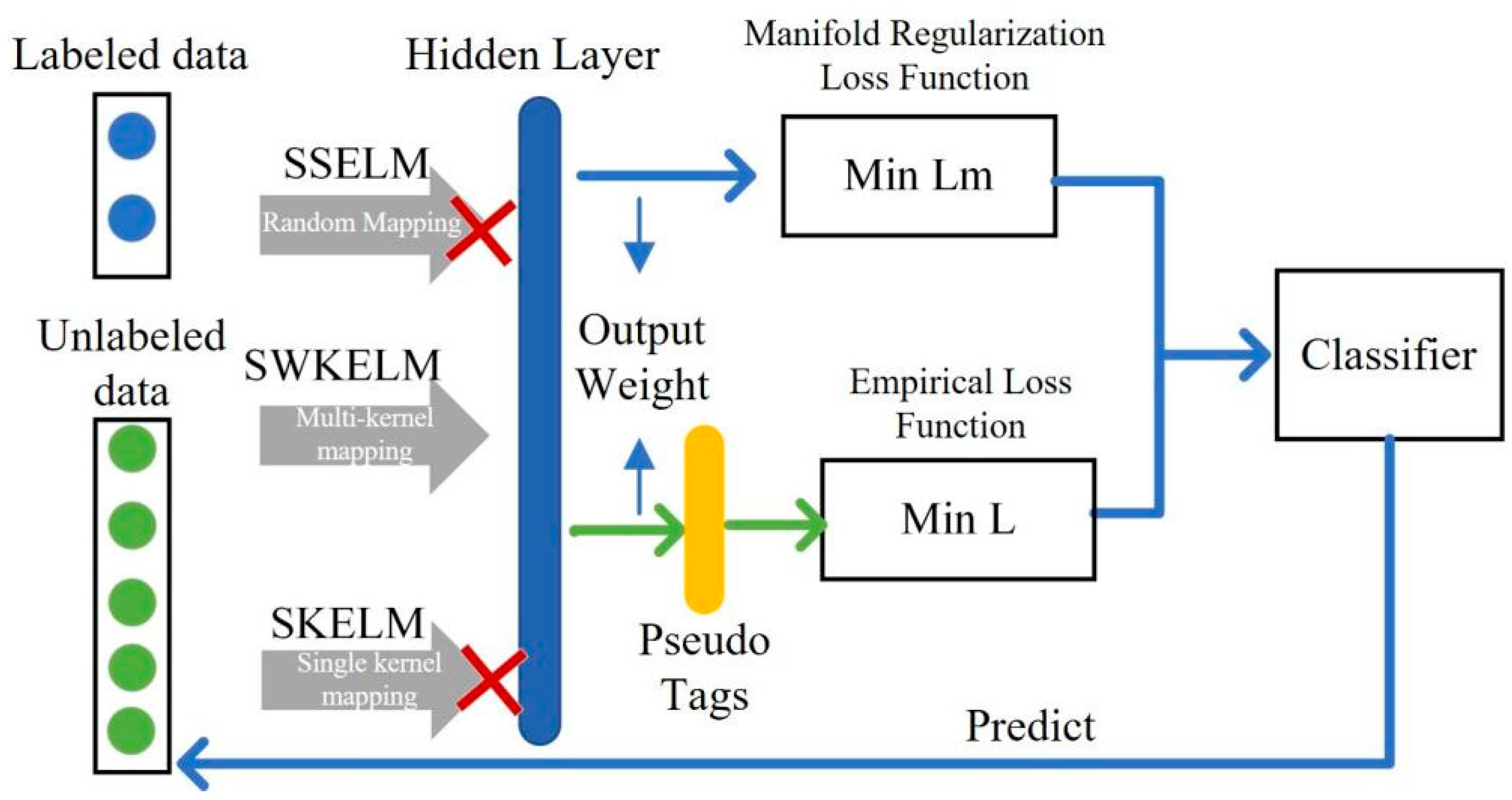
The SELMWK algorithm proposed in this study aims to use the manifold regularization method to jointly train a good-performing semi-supervised classifier on both labeled and unlabeled data. The flowchart of the algorithm is shown in Figure 2:

As can be seen from Figure 2, the most significant difference between the SELMWK algorithm and the SSELM and SKELM algorithms is the mapping method of the input data to the hidden layer. SSELM uses explicit random mapping to get hidden layers. This method has high applicability but has poor operational stability and requires a large amount of computation when mapping to high dimensions. The other two methods use kernel mapping, which belongs to implicit mapping and cannot directly calculate the hidden layer. SKELM using the single-core method, has better operational stability but lower applicability. By using the weighted kernel, SELMWK can observe the data from multiple angles and extract the key information, while the applicability and operation stability are relatively good. After obtaining the hidden layer through two constraints and minimizing the manifold regularization loss function while minimizing the empirical loss function, the trained classifier is finally obtained to test the unlabeled label data. The calculation flow of the SELMWK algorithm will be described in detail below. First, define the algorithm as an optimization problem as Equation (16):

$$\underset{\mathrm{f}ϵℱ}{\min }{\mathsf{\lambda }\mathrm{L}}_{\mathrm{m}}\left(\mathrm{f}\left(X\right)\right)+\mathrm{CL}\left(Y_L,\mathrm{f}\left(X_L\right)\right)+{\Vert f\Vert }_{\mathrm{H}}^2$$

(16)

where $\mathsf{\lambda }$ and $\mathrm{C}$ are the penalty parameters, $\mathrm{X}={\left[{\mathrm{X}}_{\mathrm{L}}^{\mathrm{T}},{\mathrm{X}}_{\mathrm{U}}^{\mathrm{T}}\right]}^{\mathrm{T}}$ is the input data, ${\mathrm{X}}_{\mathrm{L}}$ is the labeled data, ${\mathrm{X}}_{\mathrm{U}}$ is the unlabeled data, ${\mathrm{Y}}_{\mathrm{L}}$ is the real label of the labeled data, $\mathrm{f}\left(·\right)$ is the correlation map. The first term is the loss function of manifold regularization, which aims to make the predicted results more in line with the geometric structure represented by the X distribution of the input data. The second term is the empirical loss function, which aims to align the predicted results more with the actual results. The third term is a regularization term that prevents the model from overfitting.

Because the kernel mapping is a nonlinear implicit mapping, for the convenience of expressing the point after the weighted kernel mapping of the input data $\mathrm{X}$ is expressed as Equation (17):

$$H=\mathsf{\Phi }\left(X\right)$$

(17)

In the formula, $\mathrm{H}={\left[{\mathrm{H}}_{\mathrm{L}}^{\mathrm{T}},{\mathrm{H}}_{\mathrm{U}}^{\mathrm{T}}\right]}^{\mathrm{T}}$, $\mathsf{\Phi }(·)$ weighted nonlinear mapping function, because $\mathrm{K}\left({\mathrm{x}}_{\mathrm{i}},{\mathrm{x}}_{\mathrm{j}}\right)=\langle \mathsf{\Phi }\left({\mathrm{x}}_{\mathrm{i}}\right),\mathsf{\Phi }\left({\mathrm{x}}_{\mathrm{j}}\right)\rangle$, where $\langle ·\rangle$ represents the inner product of vectors, so the kernel matrix can be expressed as Equation (18):

$$K=H{H}^T$$

(18)

Since the predicted labels $\tilde{\mathrm{Y}}=\mathrm{H}\mathsf{\beta }$, $\tilde{\mathrm{Y}}={\left[{\tilde{\mathrm{Y}}}_{\mathrm{L}}^{\mathrm{T}},{\tilde{\mathrm{Y}}}_{\mathrm{U}}^{\mathrm{T}}\right]}^{\mathrm{T}}$, $\mathsf{\beta }$ is the output weight matrix of the network, the loss function of the first term manifold regularization in Equation (16), which can be written in the form of Equation (19):

$${\mathrm{L}}_{\mathrm{m}}=\mathrm{Tr}\left({\mathsf{\beta }}^T{H}^T\mathrm{L}H\mathsf{\beta }\right)$$

(19)

The second loss function in Equation (16) can be written in the form of Equation (20):

$$\mathrm{L}\left({\mathrm{Y}}_{\mathrm{L}},\mathrm{f}\left({\mathrm{X}}_{\mathrm{L}}\right)\right)={{\displaystyle \sum }}_{\mathrm{i}=1}^{{\mathrm{N}}_{\mathrm{L}}}{\Vert {\tilde{\mathrm{y}}}_{\mathrm{Li}}-{\mathrm{y}}_{\mathrm{Li}}\Vert }^2$$

(20)

where parameter ${\mathrm{N}}_{\mathrm{L}}$ is the amount of labeled data. Simplifying Equation (20), we can finally get the loss function of the second term in Equation (16), which can be rewritten in the form of Equation (21):

$$\mathrm{L}\left({\mathrm{Y}}_{\mathrm{L}},\mathrm{f}\left({\mathrm{X}}_{\mathrm{L}}\right)\right)={\Vert H_L\mathsf{\beta }-Y_L\Vert }^2$$

(21)

Bringing Equation (21) and Equation (19) into Equation (16) can finally obtain the function that needs to be optimized as Equation (22):

$$\underset{\mathsf{\beta }}{\min }\frac{\mathsf{\lambda }}{2}\mathrm{Tr}\left({\mathsf{\beta }}^T{H}^{T}LH\mathsf{\beta }\right)+\frac{{\mathrm{C}}_0}{2}{\Vert H_L\mathsf{\beta }-Y_L\Vert }^2+\frac{1}{2}{\Vert \mathsf{\beta }\Vert }^2$$

(22)

where $\mathsf{\lambda }$ and ${\mathrm{C}}_0$ are custom trade-off parameters used to balance the influence of these two parts. For the convenience of subsequent calculations, write ${\mathrm{C}}_0$ in the form of a diagonal matrix, such as Equation (23):

$${\Lambda }_C=\mathrm{dig}\left({\mathrm{C}}_0,{\mathrm{C}}_0,\cdots ,{\mathrm{C}}_0,0,\cdots ,0\right)$$

(23)

In Equation (23), the number of ${\mathrm{C}}_0$ is the number of labeled samples, and the number of $0$ is not the number of unlabeled samples. So, Equation (22) can be rewritten as Equation (24):

$$\underset{\mathsf{\beta }}{\min }\frac{\mathsf{\lambda }}{2}\mathrm{Tr}\left({\mathsf{\beta }}^T{H}^{T}LH\mathsf{\beta }\right)+\frac{1}{2}\mathrm{Tr}\left[{\left(Y^{*}-H\mathsf{\beta }\right)}^T{\Lambda }_C\left(Y^{*}-H\mathsf{\beta }\right)\right]+\frac{1}{2}{\Vert \mathsf{\beta }\Vert }^2$$

(24)

In the formula, ${\mathrm{Y}}^{*}\in {\mathrm{R}}^{\mathrm{N}}$, where the first ${\mathrm{N}}_{\mathrm{L}}$ rows are true labels with labeled data, and the rest are pseudo labels without labeled data, set to $-1$. Solving the optimization problem of Equation (24) and finding its gradient, Equation (25) can be obtained:

$$\nabla =\mathsf{\beta }+H^T{\Lambda }_C\left(H\mathsf{\beta }-Y^{*}\right)+\lambda ·H^{T}LH\mathsf{\beta }$$

(25)

Let $\nabla =0$, the output weight matrix of the network is obtained as Equation (26):

$$\mathsf{\beta }=H^T{\left({\Lambda }_{C}H{H}^T+\lambda LH{H}^T+I_N\right)}^{-1}{\Lambda }_C{Y}^{*}$$

(26)

Substituting Equation (18) into Equation (26), the form of the output weight matrix of the network can be changed to the form of Equation (27):

$$\mathsf{\beta }=H^T{\left({\Lambda }_{C}K+\lambda LK+I_N\right)}^{-1}{\Lambda }_C{Y}^{*}$$

(27)

Kernel mapping is an implicit mapping, and its specific form is not known. Therefore ${\mathrm{H}}^{\mathrm{T}}$ is not known, so $\mathsf{\beta }$ cannot be calculated. However, the network’s output can be calculated directly to skip the process of calculating β. The final output of the SELMWK algorithm is Equation (28):

$$Y_{out}=\left[\mathrm{K}\left(x_t,x_1\right),\cdots ,\mathrm{K}\left(x_t,x_N\right)\right]{\left({\Lambda }_{C}K+\lambda LK+I_N\right)}^{-1}{\Lambda }_C{Y}^{*}$$

(28)

5. Result

In this part, we mainly use two public data to conduct related experiments on data analysis and algorithm performance analysis. It is mainly divided into the following three parts: (1) The experiment of feature extraction on dataset 2; (2) The algorithm effect before and after feature extraction is analyzed and compared; (3) The comparison of SELMWK and other algorithms in recognition effect experiments. These three experiments verify the effectiveness of the SELMWK algorithm proposed in this study in solving the semi-supervised classification problem of the same domain data in machine smell.

5.1. Feature Extraction Experiment

After the cutting process of data processing, the problem of data sample data alignment is solved, and the dimension of the data is reduced to a certain extent. However, the data sample dimension is still too large, and the information is redundant, which will greatly increase the calculation in the training and testing process [30]. Directly reducing the dimension of data samples through random feature matrix mapping is likely to lose a lot of critical information. This study adopts a very good simple, and effective feature extraction method.

Table 5. Features extracted from the data curve.

Steady State Characteristics	Dynamic Features
	Adsorption stage	Desorption stage
$\Delta \mathrm{X}$	$\max \left({\mathrm{Y}}_{0.01}\right)$	$\min \left({\mathrm{Y}}_{0.01}\right)$
$\Delta {\mathrm{X}}^{*}$	$\max \left({\mathrm{Y}}_{0.001}\right)$	$\min \left({\mathrm{Y}}_{0.001}\right)$
	$\max \left({\mathrm{Y}}_{0.0001}\right)$	$\min \left({\mathrm{Y}}_{0.0001}\right)$

shows all the features extracted by this feature extraction method:

First, select the steady-state feature, the difference between the maximum data value and the baseline. The selection method is as shown in Equation (29):

$$\Delta \mathrm{X}=\underset{\mathrm{t}}{\max }\mathrm{x}\left(\mathrm{t}\right)-\underset{\mathrm{t}}{\min }\mathrm{x}\left(\mathrm{t}\right)$$

(29)

However, due to sensor drift, the maximum response and baseline of the sensor may change, so it is not enough to extract a single maximum difference. The effect of sensor drift can be reduced by comparing the differential value with the baseline so that the normalized steady-state characteristic can be expressed as Equation (30):

$$\Delta {\mathrm{X}}^{*}=\frac{\underset{\mathrm{t}}{\max }\mathrm{x}\left(\mathrm{t}\right)-\underset{\mathrm{t}}{\min }\mathrm{x}\left(\mathrm{t}\right)}{\underset{\mathrm{t}}{\min }\mathrm{x}\left(\mathrm{t}\right)}$$

(30)

where $\mathrm{x}\left(\mathrm{t}\right)$ represents the time-varying data collected by the sensor, and $\mathrm{t}$ represents the time $\mathrm{t}\in \left[0,\mathrm{T}\right]$.

The above two characteristics belong to the steady state characteristics and can only reflect the characteristics of the steady state. During the gas reaction process and desorption process, important features of the data are often preserved. In order to represent the dynamic characteristics of the sensor, a method in the field of econometrics called Exponential Moving Average (EMA) will be used. The calculation method is shown in Equation (31):

$$\mathrm{y}\left(\mathrm{t}\right)=\left(1-\mathsf{\theta }\right)\mathrm{y}\left(\mathrm{t}\right)+\mathsf{\theta }\left(\mathrm{x}\left(\mathrm{t}\right)-\mathrm{x}\left(\mathrm{t}-1\right)\right)$$

(31)

In Equation (31), $\mathrm{t}=1,2,3,\cdots \mathrm{T}$, the initial value $\mathrm{y}\left(0\right)=0$, $\mathsf{\theta }$ is the smoothing parameter, and its values are set to 0.01, 0.001, 0.0001 respectively. Figure 3 shows the exponential moving average transformed graph of the chemical sensor TGS2612 5.65V at 250 ppm methane gas, using different $\mathsf{\theta }$ parameters:

As seen in Figure 3, the graph reflects the dynamic characteristics of the sensor response curve well. The minimum and maximum values of the curve represent the maximum rate of change of the sensor resistance during the adsorption and desorption phases of the sensor array, respectively. At the same time, smoothing parameters are used to reduce the influence of resistance value fluctuations during the sensor response process. A total of three smoothing parameters were selected in this experiment to extract the maximum and minimum values of the data after exponential transformation. Therefore, each sensor has eight features, including two dynamic features and six steady-state features.

5.2. Comparative Experiment of Feature Extraction

Due to the lack of data in some samples in the original data, the original 480,000-dimensional data was not used for comparison in this experiment. The experiment is mainly carried out by comparing the cropped data and the data after feature extraction.

Table 6. Comparison of computing time before and after feature extraction (s).

Training Set Size	SVM-Linear	SVM-rbf	LDA	SELMWK
Before feature extraction
10	5.5 × 10−2	6.5 × 10−2	2.6 × 10−1	1.8 × 10−1
50	5.7 × 10−1	1.0	1.5	1.4
500	1.2	1.4	4.1	99.43
After feature extraction
10	5.1 × 10−4	4.6 × 10−4	4.6 × 10−3	1.9 × 10−3
50	6.9 × 10−4	8.4 × 10−4	6.3 × 10−3	6.3 × 10−3
500	7.8 × 10−4	1.2 × 10−3	3.6 × 10−2	1.1 × 10−1

shows the comparison of the computing time required before and after feature extraction, and

Table 7. Differences in algorithm recognition accuracy before and after feature extraction (%).

Training Set	SVM-Linear	SVM-rbf	LDA	SELMWK
10	+31.69	+38.48	+23.74	+10.2
50	+9.45	+29.09	+0.91	+8
500	+1	+6	0	+5

shows the difference in recognition accuracy before and after feature extraction:

In this experiment, three traditional machine learning methods are selected to test the effect of feature extraction, including the semi-supervised learning algorithm SELMWK proposed in this paper. Three traditional supervised learning methods are linear support vector machine (SVM-linear), support vector machine based on RBF kernel function (SVM-rbf) and LDA. The SELMWK algorithm all uses four labeled data for experiments.

Table 6 mainly analyzes the aspect of the algorithm running time. Due to the reasons of the computer itself, it cannot be guaranteed that the environment of each running is the same, so the running time will vary, but the change is not large. The data collected in this experiment is an average of 20 runs. By comparing the running time before and after feature extraction, it can be seen that the algorithm’s running time is significantly reduced. Especially for the SELMWK algorithm, the running time before and after feature extraction is 99.43 s and 0.11 s, respectively, which greatly shortens the model training time.

Table 7 analyzes the recognition accuracy of the algorithm. The purpose of feature extraction is to reduce the computational complexity of the model and to grasp the key information points in the data. The feature extraction process cannot lose too much useful information in the original data. From the results, the feature extraction method used in this paper not only does not reduce the recognition accuracy of the algorithm but also increases the recognition accuracy of the algorithm, especially when the amount of data is small.

From the above experiments, the feature extraction method used in this study is simple, effective and easy to implement. While extracting the key information of the data, the dimension of the data is greatly reduced, thereby reducing the cost of model training.

5.3. SELMWK Algorithm Effect Comparison Experiment

5.3.1. Algorithm Verification

This experiment mainly verifies the proposed SELMWK algorithm and conducts three sets of comparative experiments. The first set of comparative experiments compares the SELMWK algorithm’s recognition accuracy with three traditional supervised learning algorithms (SVM-linear, SVM-rbf and ELM) [31,32] and a semi-supervised learning algorithm SSELM algorithm. The first dataset of this set of experiments selected Batch10 data in dataset 1, and the second dataset selected dataset 2. Figure 4 shows the test results of five different algorithms on two datasets:

Figure 4a shows the effect of 5 different algorithms on Batch10. Take 1000 samples in the dataset as the test set, and test the recognition accuracy of different algorithms when the number of labeled samples = {6,12,24,48,96,192}. As can be seen from Figure 4a, in this dataset, two SVM algorithms have the lowest recognition accuracy, while another supervised learning algorithm, ELM, has achieved good results. This is because the random hidden layer of the ELM algorithm maps the data to extract the features in the data well. When observing two semi-supervised algorithms, when there is a small amount of labeled data, the recognition effect of the SELMWK algorithm used in this paper is better than that of SSELM.

Figure 4b shows the performance of 5 different algorithms on dataset 2. Take 100 data as test samples, and test the recognition effects of different algorithms when the number of labeled samples = {4,8,16,32,64,128}. The same conclusion can be drawn from the figure; the two semi-supervised learning algorithms have better results when there is only a small amount of labeled data. Among them, the SELMWK algorithm proposed in this study is based on the SSELM algorithm, obtains a stronger mapping ability through the weighted kernel, and maps the data from multiple angles. The SELMWK algorithm can extract features from data from multiple high-dimensional spaces, resulting in better recognition results.

5.3.2. Algorithm Stability Comparison

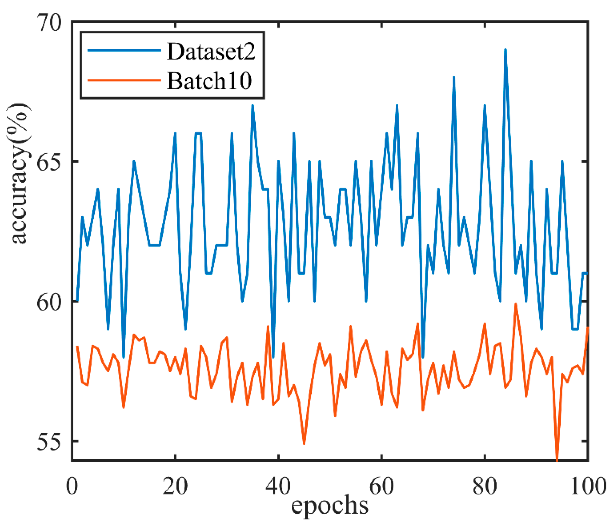
Figure 5 shows the results of the SSELM algorithm running 100 times on the above two datasets without changing any conditions. The number of labeled samples is 4 and 6, respectively:

As can be seen from Figure 5, the recognition effect of the SSELM algorithm is not stable. In Batch10, the highest recognition accuracy of the SSELM algorithm differs from the lowest recognition accuracy by about 7%. The difference between the highest and lowest recognition accuracy of the SSELM algorithm in Dataset2 is about 10%. This is because SSELM uses random hidden layer mapping, so even if the data and hyperparameters are not changed, the classifier trained by the SSELM algorithm will be different each time, so the recognition effect will continue to change. In the SELMWK algorithm, the kernel matrix is generated according to the input data after the parameters are set. The result is the same every time, so the SELMWK algorithm is more stable than the SSELM algorithm.

5.3.3. Validating the Advantages of Weighted Kernels

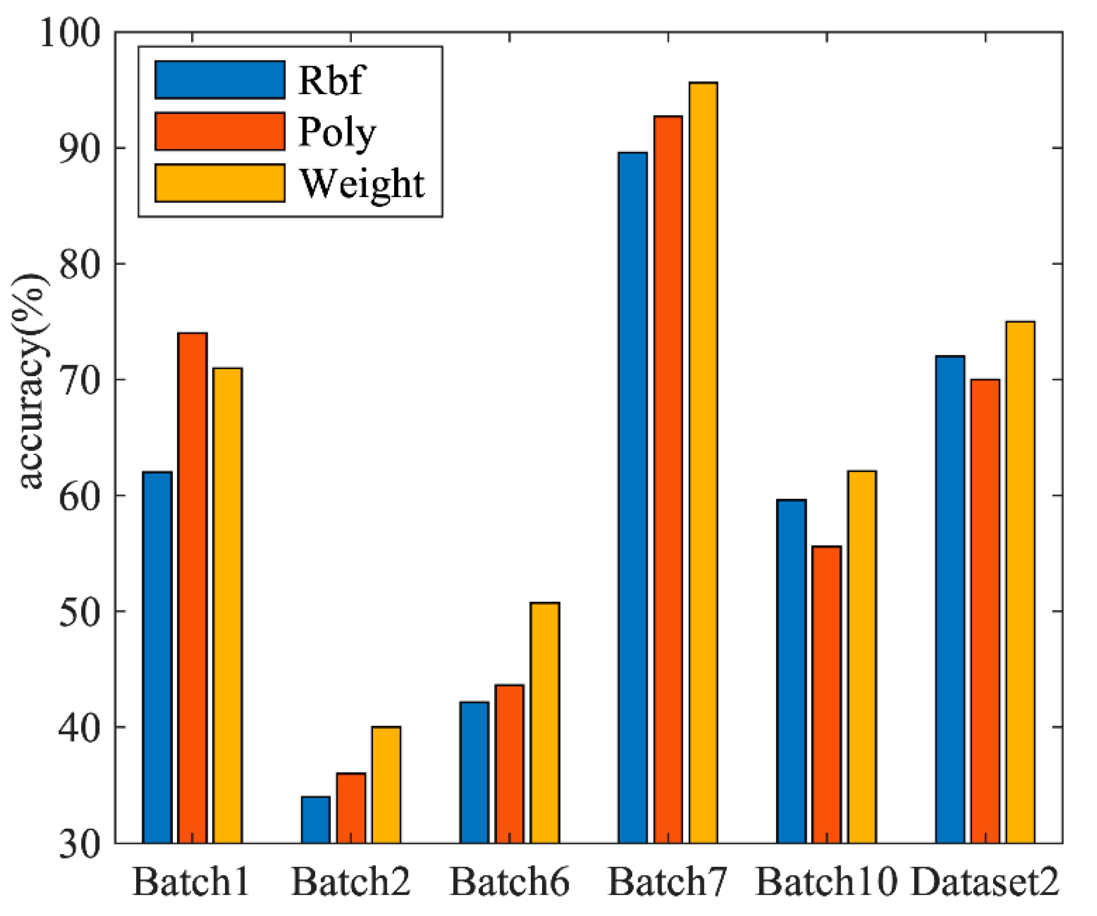
The third set of comparative experiments verifies the weighted kernel’s advantages relative to the single kernel. Figure 6 is a comparison chart of the recognition effects of the three algorithms on different data sets:

Figure 6 shows the recognition effects of the three algorithms on Batch1, Batch2, Batch6, Batch7, Batch10 and Dataset 2. Among them are six labeled data in different batch datasets in dataset 1 and four labeled data in dataset 2. It can be seen from the figure that the SELMWK using the weighted kernel function has a good recognition effect on each data set except Batch1, and the overall recognition effect is also the best. In addition, the effect of the SKELM algorithm using the RBF kernel from Batch1, Batch2, and Batch3 is lower than that of the SKELM algorithm using the Poly kernel. Especially in Batch1, it is more obvious, and the recognition accuracy differs by about 10%.

6. Discussion

The gas data collection process is cumbersome, and it is difficult to label the data, while it is relatively easy to obtain unlabeled data. In this case, this paper proposes a semi-supervised learning method based on Weighted Kernel Extreme Learning Machine (SELMWK) for the semi-supervised classification problem of the same domain data. The method combines a novel combinatorial weighted kernel with a semi-supervised kernel extreme learning machine. The model instability problem caused by the random hidden layer of the traditional semi-supervised extreme learning machine algorithm and the low generalization ability of the semi-supervised kernel extreme learning machine algorithm is improved. After verification on two public datasets, the effectiveness of the proposed algorithm is proved.

In the feature processing stage, since the experiments are carried out in the same environment, the algorithm’s running time can represent the amount of computation in the model training process. It can be seen from this that feature extraction can effectively reduce the amount of computation in the model training process. Aiming for increased recognition accuracy of the algorithm, this paper believes that this is because when the data set is small, the algorithm cannot learn the characteristics of the original gas data well, resulting in poor classification accuracy. When the amount of data increases, the algorithm gradually learns this part of the features, so the classification accuracy increases.

In the algorithm comparison experiment, two learning methods are compared. When the number of labels increases, supervised learning uses more data and learns more data features to gradually increase recognition accuracy. When the labeled data reaches 192, the recognition effects of the five algorithms are basically the same. On the other hand, when there are only a few data samples. Two graph-based semi-supervised learning methods associate labeled data with unlabeled data. Using a large amount of unlabeled data to learn the features in the data has a better recognition effect than the supervised algorithm.

In the comparative experiments of different kernel functions, using the RBF kernel has better results on the latter two datasets. This is because the SKELM algorithm that only uses a single core has higher requirements on core selection and is less applicable. The weighted kernel combines the kernel functions in a weighted way to project the data into different nonlinear spaces so that more useful information in the data can be mined, so the recognition effect is better.

7. Conclusions

The main problem solved in this study is the semi-supervised classification of data when there are only a small amount of labeled data and a large amount of unlabeled data in the same domain. The method of manifold regularization is introduced and inspired by the two algorithms of SSELM and SKELM; a new weighted kernel and SKELM are combined to propose a semi-supervised method SELMWK based on a weighted kernel extreme learning machine. And introduce it into the field of machine smell to solve the semi-supervised gas classification problem. The algorithm not only absorbs the characteristics of the fast learning rate of the SSELM algorithm but also absorbs the advantages of good stability of SKELM and improves the problem of the poor generalization ability of the single-kernel model. The algorithm is validated on two datasets and compared with four algorithms. The feature extraction method used in this study is simple, effective, and easy to implement. While extracting the key information of the data, the dimension of the data is greatly reduced, thereby reducing the cost of model training. The experimental results show that the proposed SELMWK algorithm has the best classification performance and can well solve the semi-supervised gas classification task of the same domain data on both datasets. In the best case, the recognition accuracy is 10% higher than other algorithms.

References

- Xu, M.; Wang, J.; Zhu, L. Tea quality evaluation by applying E-nose combined with chemometrics methods. J. Food Sci. Technol. 2021, 58, 1549–1561. [Google Scholar] [CrossRef] [PubMed]
- Zheng, W.; Yang, B.; Xiao, Y.; Tian, J.; Liu, S.; Yin, L. Low-Dose CT Image Post-Processing Based on Learn-Type Sparse Transform. Sensors 2022, 22, 2883. [Google Scholar] [CrossRef] [PubMed]
- Zhang, W.; Yao, G.; Yang, B.; Zheng, W.; Liu, C. Motion Prediction of Beating Heart Using Spatio-Temporal LSTM. IEEE Signal Process. Lett. 2022, 29, 787–791. [Google Scholar] [CrossRef]
- Dankwa, S.; Zheng, W. Special Issue on Using Machine Learning Algorithms in the Prediction of Kyphosis Disease: A Comparative Study. Appl. Sci. 2019, 9, 3322. [Google Scholar] [CrossRef]
- Liu, H.; Li, Q.; Yan, B.; Zhang, L.; Gu, Y. Bionic electronic nose based on MOS sensors array and machine learning algorithms used for wine properties detection. Sensors 2019, 19, 45. [Google Scholar] [CrossRef]
- Zhang, L.; Tian, F.; Liu, S.; Guo, J.; Hu, B.; Ye, Q.; Dang, L.; Peng, X.; Kadri, C.; Feng, J. Chaos based neural network optimization for concentration estimation of indoor air contaminants by an electronic nose. Sens. Actuators A Phys. 2013, 189, 161–167. [Google Scholar] [CrossRef]
- Zhang, Z.; Liu, Y.; Tian, J.; Liu, S.; Yang, B.; Xiang, L.; Yin, L.; Zheng, W. Study on Reconstruction and Feature Tracking of Silicone Heart 3D Surface. Sensors 2021, 21, 7570. [Google Scholar] [CrossRef]
- Tang, Y.; Liu, S.; Deng, Y.; Zhang, Y.; Yin, L.; Zheng, W. Construction of force haptic reappearance system based on Geomagic Touch haptic device. Comput. Methods Programs Biomed. 2020, 190, 105344. [Google Scholar] [CrossRef]
- Yang, B.; Liu, C.; Zheng, W.; Liu, S.; Huang, K. Reconstructing a 3D heart surface with stereo-endoscope by learning eigen-shapes. Biomed. Opt. Express 2018, 9, 6222–6236. [Google Scholar] [CrossRef]
- Yang, B.; Liu, C.; Huang, K.; Zheng, W. A triangular radial cubic spline deformation model for efficient 3D beating heart tracking. Signal Image Video Process. 2017, 11, 1329–1336. [Google Scholar] [CrossRef]
- VA, B.; Subramoniam, M.; Mathew, L. Noninvasive detection of COPD and Lung Cancer through breath analysis using MOS Sensor array based e-nose. Expert Rev. Mol. Diagn. 2021, 21, 1223–1233. [Google Scholar] [CrossRef] [PubMed]
- Hendrick, H.; Hidayat, R.; Horng, G.J.; Wang, Z.H. Non-invasive method for tuberculosis exhaled breath classification using electronic nose. IEEE Sens. J. 2021, 21, 11184–11191. [Google Scholar] [CrossRef]
- Zhu, X.; Goldberg, A.B. Introduction to semi-supervised learning. Synth. Lect. Artif. Intell. Mach. Learn. 2009, 3, 1–130. [Google Scholar]
- Wu, B.; Meng, D.; Zhao, H. Semi-Supervised Learning for Seismic Impedance Inversion Using Generative Adversarial Net-works. Remote Sens. 2021, 13, 909. [Google Scholar] [CrossRef]
- Rostami, M.; Kolouri, S.; Eaton, E.; Kim, K. Deep Transfer Learning for Few-Shot SAR Image Classification. Remote Sens. 2019, 11, 1374. [Google Scholar] [CrossRef]
- Wei, D.; Du, Y.; Du, L.; Li, L. Target Detection Network for SAR Images Based on Semi-Supervised Learning and Attention Mechanism. Remote Sens. 2021, 13, 2686. [Google Scholar] [CrossRef]
- Zhang, B.; Ye, H.; Yu, G.; Wang, B.; Wu, Y.; Fan, J.; Chen, T. Sample-Centric Feature Generation for Semi-Supervised Few-Shot Learning. IEEE Trans. Image Process. 2022, 31, 2309–2320. [Google Scholar] [CrossRef]
- Yarowsky, D. Unsupervised word sense disambiguation rivaling supervised methods. In Proceedings of the 33rd Annual Meeting of the Association for Computational Linguistics, Cambridge, MA, USA, 26–30 June 1995; pp. 189–196. [Google Scholar]
- Li, X.; Lu, P.; Hu, L.; Wang, X.; Lu, L. A novel self-learning semi-supervised deep learning network to detect fake news on social media. Multimed. Tools Appl. 2021, 81, 19341–19349. [Google Scholar] [CrossRef]
- Blum, A.; Mitchell, T. Combining labeled and unlabeled data with co-training. In Proceedings of the Eleventh Annual Conference on Computational Learning Theory, Madison, WI, USA, 24–26 July 1998; pp. 92–100. [Google Scholar]
- Yaslan, Y.; Cataltepe, Z. Co-training with relevant random subspaces. Neurocomputing 2010, 73, 1652–1661. [Google Scholar] [CrossRef]
- Qiao, S.; Shen, W.; Zhang, Z.; Wang, B.; Yuille, A. Deep co-training for semi-supervised image recognition. In Proceedings of the European Conference on Computer Vision (ECCV), Munich, Germany, 8–14 September 2018; pp. 135–152. [Google Scholar]
- Joachims, T. Transductive Inference for Text Classification Using Support Vector Machines; Universität Dortmund: Dortmund, Germany, 1999; pp. 200–209. [Google Scholar]
- Zemmal, N.; Azizi, N.; Dey, N.; Sellami, M. Adaptive semi supervised support vector machine semi supervised learning with features cooperation for breast cancer classification. J. Med. Imaging Health Inform. 2016, 6, 53–62. [Google Scholar] [CrossRef]
- Zhang, L.; Zhang, D.; Yin, X.; Liu, Y. A novel semi-supervised learning approach in artificial olfaction for E-nose application. IEEE Sens. J. 2016, 16, 4919–4931. [Google Scholar] [CrossRef]
- Vergara, A.; Vembu, S.; Ayhan, T.; Ryan, M.A.; Homer, M.L.; Huerta, R. Chemical gas sensor drift compensation using classifier ensembles. Sens. Actuators B Chem. 2012, 166, 320–329. [Google Scholar] [CrossRef]
- Rodriguez-Lujan, I.; Fonollosa, J.; Vergara, A.; Homer, M.; Huerta, R. On the calibration of sensor arrays for pattern recognition using the minimal number of experiments. Chemom. Intell. Lab. Syst. 2014, 130, 123–134. [Google Scholar] [CrossRef]
- Fonollosa, J.; Fernandez, L.; Gutiérrez-Gálvez, A.; Huerta, R.; Marco, S. Calibration transfer and drift counteraction in chemical sensor arrays using Direct Standardization. Sens. Actuators B Chem. 2016, 236, 1044–1053. [Google Scholar] [CrossRef]
- Gönen, M.; Alpaydın, E. Multiple kernel learning algorithms. J. Mach. Learn. Res. 2011, 12, 2211–2268. [Google Scholar]
- Li, Y.; Zheng, W.; Liu, X.; Mou, Y.; Yin, L.; Yang, B. Research and improvement of feature detection algorithm based on FAST. Rend. Lince 2021, 32, 775–789. [Google Scholar] [CrossRef]
- Chauhan, V.K.; Dahiya, K.; Sharma, A. Problem formulations and solvers in linear SVM: A review. Artif. Intell. Rev. 2019, 52, 803–855. [Google Scholar] [CrossRef]
- Ding, S.; Zhao, H.; Zhang, Y.; Xu, X.; Nie, R. Extreme learning machine: Algorithm, theory and applications. Artif. Intell. Rev. 2015, 44, 103–115. [Google Scholar] [CrossRef]