
An Improved Algorithm of Drift Compensation for Olfactory Sensors
 , , , and
Abstract
:1. Introduction
2. Datasets
3. Materials and Methods
3.1. Maximum Average Discrepancy
3.2. Sensor Drift Compensation Algorithm
4. Results
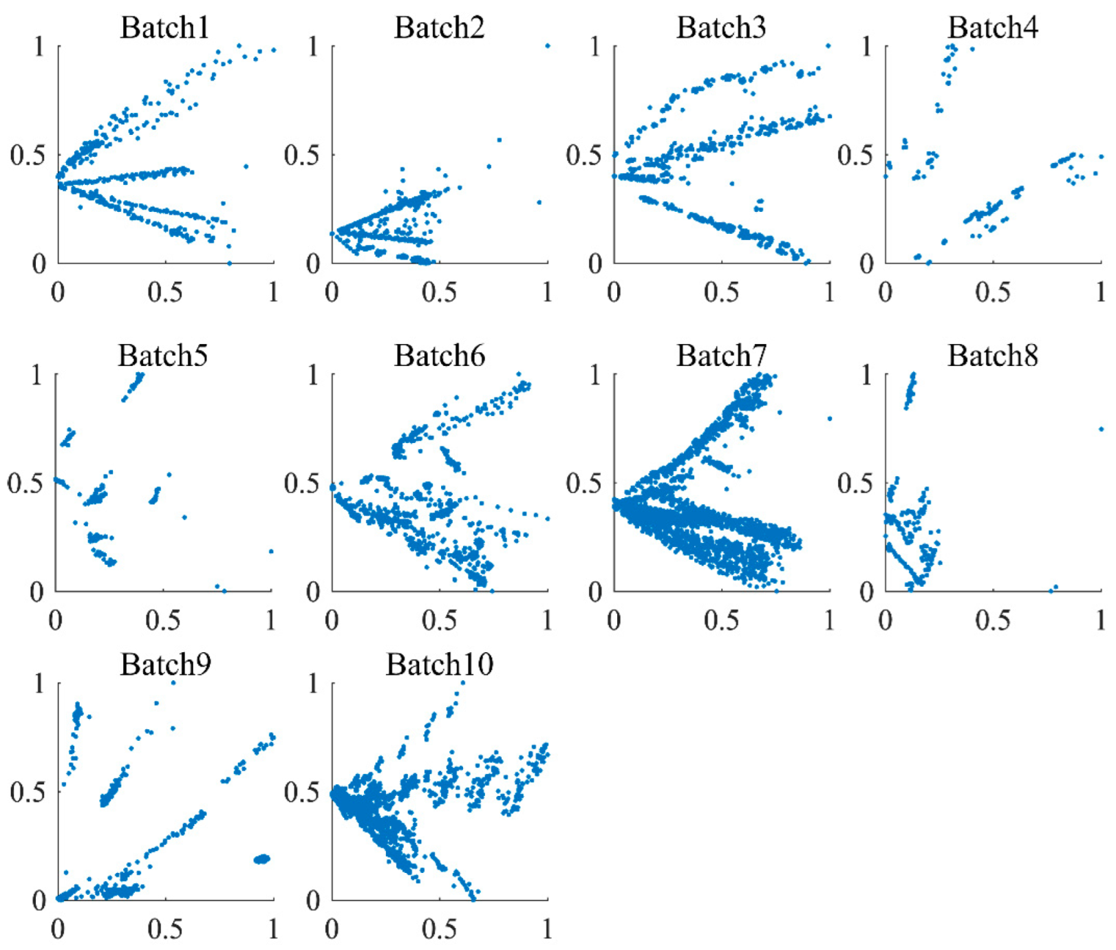
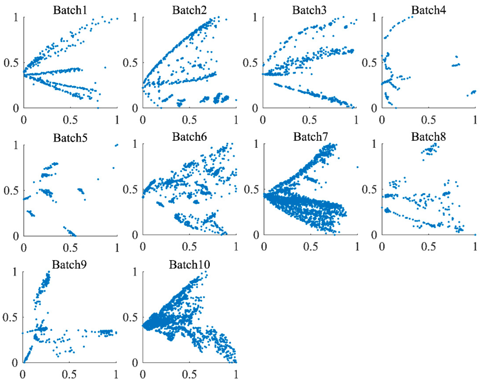
4.1. Experimental Data Distribution Analysis
4.2. Sensor Drift Algorithm Comparison Experiment
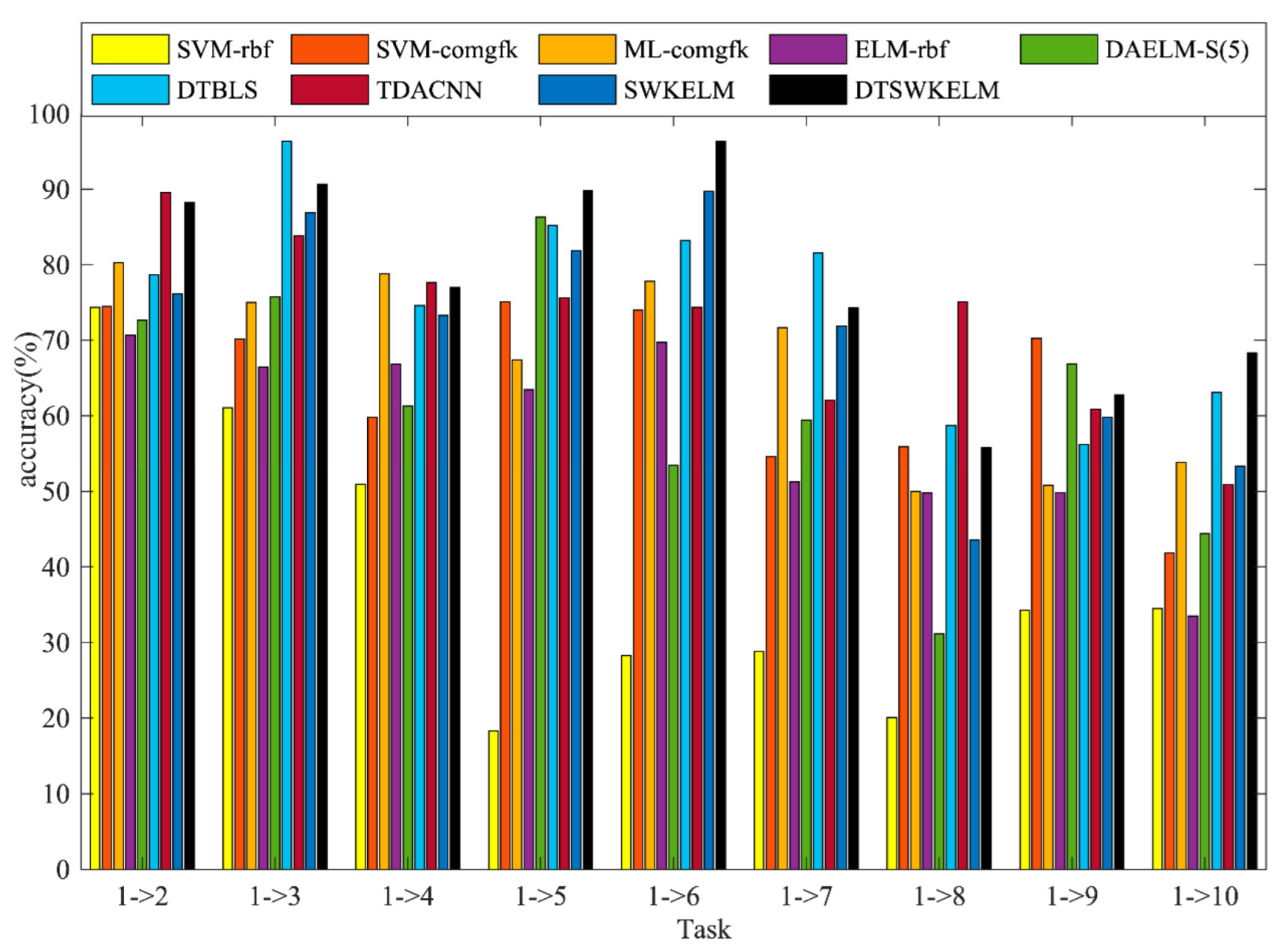
4.2.1. Experiment 1
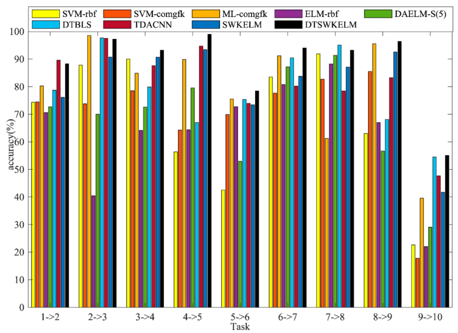
4.2.2. Experiment 2
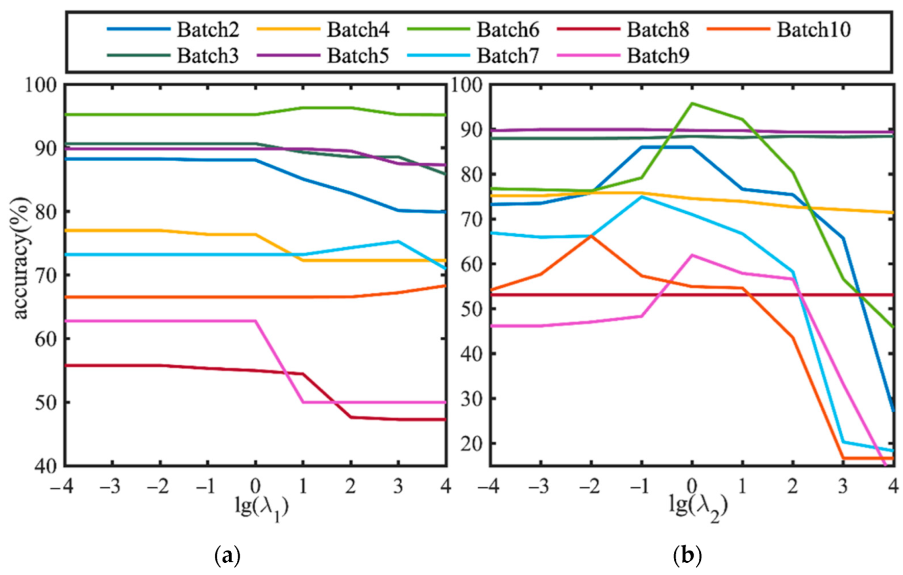
4.3. Parameter Influence and Analysis
5. Discussion
6. Conclusions
Author Contributions
Funding
Institutional Review Board Statement
Informed Consent Statement
Data Availability Statement
Conflicts of Interest
References
- Wakhid, S.; Sarno, R.; Sabilla, S.I. The effect of gas concentration on detection and classification of beef and pork mixtures using E-nose. Comput. Electron. Agric. 2022, 195, 106838. [Google Scholar] [CrossRef]
- Oates, M.J.; González-Teruel, J.D.; Ruiz-Abellon, M.C.; Guillamon-Frutos, A.; Ramos, J.A.; Torres-Sánchez, R. Using a Low-Cost Components e-Nose for Basic Detection of Different Foodstuffs. IEEE Sens. J. 2022, 22, 13872–13881. [Google Scholar] [CrossRef]
- Huang, C.; Gu, Y. A Machine Learning Method for the Quantitative Detection of Adulterated Meat Using a MOS-Based E-Nose. Foods 2022, 11, 602. [Google Scholar] [CrossRef] [PubMed]
- Alagoz, B.B.; Simsek, O.I.; Ari, D.; Tepljakov, A.; Petlenkov, E.; Alimohammadi, H. An Evolutionary Field Theorem: Evolutionary Field Optimization in Training of Power-Weighted Multiplicative Neurons for Nitrogen Oxides-Sensitive Electronic Nose Applications. Sensors 2022, 22, 3836. [Google Scholar] [CrossRef] [PubMed]
- Ari, D.; Alagoz, B.B. An effective integrated genetic programming and neural network model for electronic nose calibration of air pollution monitoring application. Neural. Comput. Applic. 2022, 34, 12633–12652. [Google Scholar] [CrossRef]
- Sarno, R.; Inoue, S.; Ardani, M.S.; Purbawa, D.P.; Sabilla, S.I.; Sungkono, K.R.; Fatichah, C.; Sunaryono, D.; Bakhtiar, A.; Prakoeswa, C.R. Detection of Infectious Respiratory Disease Through Sweat from Axillary Using an E-Nose With Stacked Deep Neural Network. IEEE Access 2022, 10, 51285–51298. [Google Scholar] [CrossRef]
- Holmberg, M.; Artursson, T. Drift Compensation, Standards, and Calibration Methods; Wiley-VCH Verlag GmbH & Co. KGaA: Weinheim, Germany, 2004. [Google Scholar]
- Schöberl, M.; Fößel, S.; Kaup, A. Fixed pattern noise column drift compensation (CDC) for digital moving picture cameras. In Proceedings of the IEEE International Conference on Image Processing, Hong Kong, 26–29 September 2010; IEEE: New York, NY, USA, 2010. [Google Scholar]
- Ahmadou, D.; Laref, R.; Losson, E.; Siadat, M. Reduction of drift impact in gas sensor response to improve quantitative odor analysis. In Proceedings of the 2017 IEEE International Conference on Industrial Technology (ICIT), Toronto, Canada, 22–25 March 2017; IEEE: New York, NY, USA, 2017. [Google Scholar]
- Hang, L.; Chu, R.; Jian, R.; Xia, J. Long-term drift compensation algorithms based on the kernel-orthogonal signal correction in electronic nose systems. In Proceedings of the International Conference on Fuzzy Systems & Knowledge Discovery, Zhangjiajie, China, 15–17 August 2015; IEEE: New York, NY, USA, 2016. [Google Scholar]
- Whslén, J.; Orhan, I.; Sturm, D.; Lindh, T. Performance evaluation of time synchronization and clock drift compensation in wireless personal area networks. In Proceedings of the 7th International Conference on Body Area Networks, Oslo, Norway, 24–26 September 2012. [Google Scholar]
- Tao, Y.; Zeng, K.; Liang, Z. Drift compensation algorithm based on Time-Wasserstein dynamic distribution alignment. In Proceedings of the 2020 IEEE/CIC International Conference on Communications in China (ICCC), Xiamen, China, 28–30 July 2020; pp. 130–135. [Google Scholar] [CrossRef]
- Wold, S.; Antti, H.; Lindgren, F.; Öhman, J. Orthogonal signal correction of near-infrared spectra. Chemom. Intell. Lab. Syst. 1998, 44, 175–185. [Google Scholar] [CrossRef]
- Feng, J.; Tian, F.; Jia, P.; He, Q.; Shen, Y.; Fan, S. Improving the performance of electronic nose for wound infection detection using orthogonal signal correction and particle swarm optimization. Sens. Rev. 2014, 2014, 34. [Google Scholar] [CrossRef]
- Artursson, T.; Eklöv, T.; Lundström, I.; Mårtensson, P.; Sjöström, M.; Holmberg, M. Drift correction for gas sensors using multivariate methods. J. Chemom. A J. Chemom. Soc. 2000, 14, 711–723. [Google Scholar] [CrossRef]
- Yan, J.; Chen, F.; Liu, T.; Zhang, Y.; Peng, X.; Yi, D.; Duan, S. Subspace alignment based on an extreme learning machine for electronic nose drift compensation. Knowl. Based Syst. 2022, 235, 107664. [Google Scholar] [CrossRef]
- Ma, Z.; Luo, G.; Qin, K.; Wang, N.; Niu, W. Online Sensor Drift Compensation for E-Nose Systems Using Domain Adaptation and Extreme Learning Machine. Sensors 2018, 18, 742. [Google Scholar]
- Distante, C.; Siciliano, P.; Vasanelli, L. Odor discrimination using adaptive resonance theory. Sens. Actuators B Chem. 2000, 69, 248–252. [Google Scholar] [CrossRef]
- Zuppa, M.; Distante, C.; Siciliano, P.; Persaud, K.C. Drift counteraction with multiple self-organising maps for an electronic nose. Sens. Actuators B: Chem. 2004, 98, 305–317. [Google Scholar] [CrossRef]
- Liang, Z.; Zhang, L.; Tian, F.; Wang, C.; Yang, L.; Guo, T.; Xiong, L. A novel WWH problem-based semi-supervised online method for sensor drift compensation in E-nose. Sens. Actuators B Chem. 2021, 349, 130727. [Google Scholar] [CrossRef]
- Das, P.; Manna, A.; Ghoshal, S. Gas sensor drift compensation by ensemble of classifiers using extreme learning machine. In Proceedings of the International Conference on Renewable Energy Integration into Smart Grids: A Multidisciplinary Approach to Technology Modelling and Simulation (ICREISG), Bhubaneswar, India, 14–15 February 2020. [Google Scholar]
- Vergara, A.; Vembu, S.; Ayhan, T.; Ryan, M.A.; Homer, M.L.; Huerta, R. Chemical gas sensor drift compensation using classifier ensembles. Sens. Actuators B Chem. 2012, 166, 320–329. [Google Scholar] [CrossRef]
- Liu, Q.; Li, X.; Ye, M.; Ge, S.S.; Du, X. Drift compensation for electronic nose by semi-supervised domain adaption. IEEE Sens. J. 2013, 14, 657–665. [Google Scholar] [CrossRef]
- Jian, Y.; Lu, K.; Deng, C.; Wen, T.; Yan, J. Drift compensation for e-nose using qpso-based domain adaptation kernel elm. In International Symposium on Neural Networks (ISNN2018); Springer: Cham, Switzerland, 2018. [Google Scholar]
- Guo, T.; Yu, K.; Cheng, X.; Bashir, A.K. Robust electronic nose in industrial cyber physical systems based on domain adaptive subspace transfer model. In Proceedings of the 2021 IEEE International Conference on Communications Workshops (ICC Workshops), Montreal, QC, Canada, 14–23 June 2021; IEEE: New York, NY, USA, 2021. [Google Scholar]
- Liu, R.; Chen, X.; Tian, F.; Qian, J.; Wang, F.; Yi, L. MCSP-SSS: A Domain Adaptive Framework for High-Accuracy Sensor Data Classification. IEEE Sens. J. 2021, 21, 25995–26005. [Google Scholar] [CrossRef]
- Zhang, L.; Zhang, D. Domain adaptation extreme learning machines for drift compensation in E-nose systems. IEEE Trans. Instrum. Meas. 2014, 64, 1790–1801. [Google Scholar] [CrossRef]
- Rodriguez-Lujan, I.; Fonollosa, J.; Vergara, A.; Homer, M.; Huerta, R. On the calibration of sensor arrays for pattern recognition using the minimal number of experiments. Chemom. Intell. Lab. Syst. 2014, 130, 123–134. [Google Scholar] [CrossRef]
- Borgwardt, K.M.; Gretton, A.; Rasch, M.J.; Kriegel, H.P.; Schölkopf, B.; Smola, A.J. Integrating structured biological data by kernel maximum mean discrepancy. Bioinformatics 2006, 22, e49–e57. [Google Scholar] [CrossRef] [Green Version]
- Liu, B.; Zeng, X.; Tian, F.; Zhang, S.; Zhao, L. Domain transfer broad learning system for long-term drift compensation in electronic nose systems. IEEE Access 2019, 7, 143947–143959. [Google Scholar] [CrossRef]
- Zhang, Y.; Xiang, S.; Wang, Z.; Peng, X.; Tian, Y.; Duan, S.; Yan, J. TDACNN: Target-domain-free domain adaptation convolutional neural network for drift compensation in gas sensors. Sens. Actuators B Chem. 2022, 361, 131739. [Google Scholar] [CrossRef]


| Batch ID | Month | Acetone | Acetaldehyde | Ethanol | Ethylene | Ammonia | Toluene | Total |
|---|---|---|---|---|---|---|---|---|
| Batch 1 | 1–2 | 90 | 98 | 83 | 30 | 70 | 74 | 445 |
| Batch 2 | 3–10 | 164 | 334 | 100 | 109 | 532 | 5 | 1244 |
| Batch 3 | 11–13 | 365 | 490 | 216 | 240 | 275 | 0 | 1586 |
| Batch 4 | 14,15 | 64 | 43 | 12 | 30 | 12 | 0 | 161 |
| Batch 5 | 16 | 28 | 40 | 20 | 46 | 63 | 0 | 197 |
| Batch 6 | 17–20 | 514 | 574 | 110 | 29 | 606 | 467 | 2300 |
| Batch 7 | 21 | 649 | 662 | 360 | 744 | 630 | 568 | 3613 |
| Batch 8 | 22,23 | 30 | 30 | 40 | 33 | 143 | 18 | 294 |
| Batch 9 | 24,30 | 61 | 55 | 100 | 75 | 78 | 101 | 470 |
| Batch10 | 36 | 600 | 600 | 600 | 600 | 600 | 600 | 3600 |
| Task | 1–>2 | 1–>3 | 1–>4 | 1–>5 | 1–>6 | 1–>7 | 1–>8 | 1–>9 | 1–>10 | AVG |
|---|---|---|---|---|---|---|---|---|---|---|
| SVM-rbf | 74.36 | 61.03 | 50.93 | 18.27 | 28.26 | 28.81 | 20.07 | 34.26 | 34.48 | 38.94 |
| SVM-comgfk | 74.47 | 70.15 | 59.78 | 75.09 | 73.99 | 54.59 | 55.88 | 70.23 | 41.85 | 64 |
| ML-comgfk | 80.25 | 74.99 | 78.79 | 67.41 | 77.82 | 71.68 | 49.96 | 50.79 | 53.79 | 67.28 |
| ELM-rbf | 70.63 | 66.44 | 66.83 | 63.45 | 69.73 | 51.23 | 49.76 | 49.83 | 33.5 | 57.93 |
| DAELM-S(5) | 72.66 | 75.72 | 61.3 | 86.29 | 53.45 | 59.4 | 31.16 | 66.85 | 44.39 | 61.25 |
| DTBLS | 78.67 | 96.36 | 74.6 | 85.23 | 83.2 | 81.53 | 58.67 | 56.19 | 63.1 | 75.28 |
| TDACNN | 89.56 | 83.83 | 77.64 | 75.63 | 74.36 | 62.08 | 75.1 | 60.85 | 50.88 | 72.21 |
| SWKELM | 76.13 | 86.88 | 73.29 | 81.82 | 89.73 | 71.88 | 43.57 | 59.78 | 53.31 | 70.71 |
| DTSWKELM | 88.26 | 90.66 | 77.01 | 89.85 | 96.31 | 74.29 | 55.78 | 62.77 | 68.33 | 78.14 |
| Task | 1–>2 | 2–>3 | 3–>4 | 4–>5 | 5–>6 | 6–>7 | 7–>8 | 8–>9 | 9–>10 | AVG |
|---|---|---|---|---|---|---|---|---|---|---|
| SVM-rbf | 74.36 | 87.83 | 90.06 | 56.35 | 42.52 | 83.53 | 91.84 | 62.98 | 22.64 | 68.01 |
| SVM-comgfk | 74.47 | 73.75 | 78.51 | 64.26 | 69.97 | 77.69 | 82.69 | 85.53 | 17.76 | 69.40 |
| ML-comgfk | 80.25 | 98.55 | 84.89 | 89.85 | 75.53 | 91.17 | 61.22 | 95.53 | 39.56 | 79.62 |
| ELM-rbf | 70.63 | 40.44 | 64.16 | 64.37 | 72.7 | 80.75 | 88.2 | 67 | 22 | 63.36 |
| DAELM-S(5) | 72.66 | 69.99 | 72.61 | 79.54 | 52.93 | 87.18 | 91.36 | 56.66 | 29.05 | 68 |
| DTBLS | 78.67 | 97.65 | 79.88 | 67.01 | 75.34 | 90.44 | 95.1 | 68.09 | 54.47 | 78.52 |
| TDACNN | 89.56 | 97.46 | 87.58 | 94.68 | 73.9 | 80.18 | 78.43 | 83.19 | 47.64 | 81.48 |
| SWKELM | 76.13 | 90.73 | 90.68 | 93.4 | 73.43 | 83.73 | 87.07 | 92.55 | 41.69 | 81.05 |
| DTSWKELM | 88.26 | 97.23 | 93.17 | 98.98 | 78.43 | 93.99 | 93.19 | 96.38 | 55.08 | 88.30 |
Publisher’s Note: MDPI stays neutral with regard to jurisdictional claims in published maps and institutional affiliations. |
© 2022 by the authors. Licensee MDPI, Basel, Switzerland. This article is an open access article distributed under the terms and conditions of the Creative Commons Attribution (CC BY) license (https://creativecommons.org/licenses/by/4.0/).
Share and Cite
Lu, S.; Guo, J.; Liu, S.; Yang, B.; Liu, M.; Yin, L.; Zheng, W. An Improved Algorithm of Drift Compensation for Olfactory Sensors. Appl. Sci. 2022, 12, 9529. https://doi.org/10.3390/app12199529
Lu S, Guo J, Liu S, Yang B, Liu M, Yin L, Zheng W. An Improved Algorithm of Drift Compensation for Olfactory Sensors. Applied Sciences. 2022; 12(19):9529. https://doi.org/10.3390/app12199529
Chicago/Turabian StyleLu, Siyu, Jialiang Guo, Shan Liu, Bo Yang, Mingzhe Liu, Lirong Yin, and Wenfeng Zheng. 2022. "An Improved Algorithm of Drift Compensation for Olfactory Sensors" Applied Sciences 12, no. 19: 9529. https://doi.org/10.3390/app12199529