
Post-Buckling Behaviour of Steel Structures with Different Types of Imperfections


Faculty of Civil and Transport Engineering, Poznan University of Technology, Piotrowo 5, 60-965 Poznań, Poland
Appl. Sci. 2022, 12(18), 9018; https://doi.org/10.3390/app12189018
Submission received: 25 July 2022
/
Revised: 4 September 2022
/
Accepted: 5 September 2022
/
Published: 8 September 2022
(This article belongs to the Special Issue Steel Structures Design and Evaluation in Building Engineering)
Abstract
:In this paper, the stability of steel members with a complex initial geometrical imperfection pattern are analysed. This issue is extremely important in the case of slender structures, characterised by multiple close critical loads and modal interactions, which can lead to unstable post-critical paths and imperfection sensitivity. Despite the fact that the loss of stability, as a result of complex geometrical imperfections, is a very common mechanism for the destruction of slender steel structures, there is still no unambiguous and adequate research in the literature and in scientific research taking into account multimodal buckling. Therefore, in this study, special attention was focused on the analysis of the equilibrium path of the structure in the pre- and post-buckling range. This was studied by introducing a model of a structure composed of four rigid bars connected by elastic nodes. For this model, as well as for the structure with and without initial geometrical imperfections, a set of nonlinear algebraic equations of equilibrium was developed. A complex pattern of imperfections was taken into account using a linear superposition of buckling modes obtained from a linear eigenvalue problem. In order to investigate the nature of bifurcation points, the concept of minimum of potential energy was adopted. By means of numerous examples, the influence of imperfections on the structural behaviour was discussed. It was found that, for special imperfection patterns, an increase in the amplitude of initial geometrical imperfection can result in an increase in the value of the critical load defining the bifurcation point. In these cases, initial geometrical imperfections can play a positive role, resulting in stable post-buckling behaviour. This phenomenon corresponds with the so-called “modal nudging” which aims to improve the buckling response of slender elastic structures by introducing a small disturbance in the primary geometry of the structure, which results in equilibrium paths of greater load-carrying capacity. Among other observations, a snap-through phenomenon caused by transition from the local to the global minimum of potential energy was also noted. The observed snap-through was caused by the specific configuration of initial geometrical imperfections, which in this case played quite a dangerous role. It should be emphasised that the proposed model structure allows for a full description of the post-critical behaviour and a trace of the influence of complex imperfection configurations in a simple and clear manner.
1. Introduction
In order to understand the essence of the work of steel bar structures, it is worth going back to the beginnings related to their mechanics. In the case of a slender bar, the most typical failure mechanism is loss of stability. In general, the stability of a structure can be defined as a phenomenon in which a slight disturbance causes a very large change. Depending on the effect of the disturbance, the condition of the structure can be defined as stable or unstable. Usually, such a definition is referred to as stability in Lyapunov’s meaning. Another approach to the analysis of the equilibrium states of the structure is based on the potential energy analysis. It is assumed that the structure is in equilibrium when potential energy reaches a minimum. The necessary condition for the occurrence of minimum potential energy is the disappearance of its first variation. The nature of the equilibrium path is determined by higher order variations of potential energy. The type of bifurcation point can be defined based on the analysis of the second variation of potential energy. This approach was proposed by Stepan Timoshenko [1], who was considered to be the father of modern engineering mechanics. In the classical theory of stability, the type of equilibrium path can be illustrated by a ball moving on a differently shaped surface as stable, unstable and neutral. In problems with many degrees of freedom, there is also another case, called the metastable point of equilibrium. This state is characterised by temporary equilibrium and local minimum of potential energy. Note that the nature of a bifurcation point can be defined by the higher-order variation of potential energy and can be symmetric or asymmetric.
In engineering practice, i.e., in the current codes [2], the most common concept is the one of critical stress, which was proposed originally by the Swiss mathematician Leonhard Euler, who in 1757 derived the formula of critical load. This formula describes the compressive load at which, due to initial geometrical imperfection, a slender column suddenly bends. This phenomenon is called buckling and can take different forms with respect to the bar cross-sectional characteristic. In case of slender, thin-walled bar members, a spatial loss of stability is observed. In the profile, warping occurs, combined with elastic couplings involving bending and torsion. Vasilii Zakharovich Vlasov developed a torsion theory in which restrained warping is included [3]. This theory is also called “warping torsion” or “non-uniform torsion”. Note that the loss of stability is limited by the occurrence of initial geometrical imperfections. In typical structural elements, geometrical imperfections can take global and local forms. Global imperfections refer mainly to the bending or twisting of rod axes. On the other hand, local imperfections may occur in the form of deviations of the dimensions of individual cross-sectional walls, or the shape of the contour of the cross-section associated with the local deformation of walls, or the symmetric and asymmetric “opening” and “closing” of the cross-section. These imperfections are particularly dangerous when their shape coincides with particular forms of the local or distortion buckling mode [4]. Taking into account the actual geometrical imperfections, both global and local, is possible using the finite element method [5,6]. Issues connected with the accuracy of the computational models which take into account the initial geometrical imperfections and residual stresses were dealt with in [7]. The influence of local geometrical imperfections of thin-walled sections on the stability of columns and short beams was analysed in [8]. There are many methods of introducing geometrical imperfections into the FEM numerical model. One of the simplest methods is the equivalent load method in which the force induces in the numerical model deformation corresponding to initial geometrical imperfections [9,10]. This method is especially suitable for generating global geometrical imperfections, but its disadvantage is the creation of additional stresses, which in fact are not accompanied by the formation of geometrical imperfections. An alternative method of imperfection modelling is a concept based on the equivalent bar stiffness proposed by [11]. In [12] the author shows that geometrically exact beam finite elements can be successfully employed to determine, accurately, the behaviour of steel I-section beams undergoing large displacements and finite rotations. For this purpose, a two-node, geometrically exact, beam element was presented and validated, which can handle arbitrary initial configurations (e.g., curved configurations), plasticity, geometric imperfections and residual stresses. A very realistic model of construction imperfections, both global and local, can be obtained by introducing a distorted geometry of the FE mesh by measuring the actual imperfections “in situ”. This approach requires the use of highly advanced measuring devices (such as 3D scanners) to create 3D imperfection maps and convert them to FEM programs. Unfortunately, in the case of civil engineering structures, this method is still rarely used because of a relatively high cost. It has one more drawback, namely it allows the creation of an initial imperfections pattern only for a given structural element. Therefore, it only covers one particular case. Due to the high randomness of imperfections, the results obtained on the basis of deterministically defined imperfections are not always reliable and do not allow potentially dangerous configurations to be identified. An alternative method of taking into account imperfections may be a method of shaping deformed geometry as a linear superposition of buckling modes obtained from a linear solution of the eigenvalue problem [13]. In this approach, the amplitude of buckling modes can be scaled by proportional coefficient factors determined arbitrarily based on standard tolerances or on a limited number of measurements of real imperfections.
Nonlinear FE formulations based on von Kármán kinematics with initial geometrical imperfections are taken into account in [14]. The authors proposed a predictor–corrector reduced-order modelling method for the nonlinear buckling analysis of thin-walled structures with initial geometrical imperfections based on Koiter theory. The main innovation of this method is the implementation of initial geometrical imperfection, instead of equivalent loads. This makes the Koiter–Newton reduced-order modelling method applicable for pre- and post-buckling, even for relatively large imperfection amplitudes.
The idea of increasing buckling capacity with modal geometrical imperfections was discussed by [15]. They note that not all imperfections are detrimental to buckling problems. A recent design trend called “modal nudging” takes advantage of geometrical imperfections to change the primary structure to equilibrium paths with greater bearing capacity. In this article, the authors proposed an automated procedure based on a Koiter-inspired reduced-order model that allows the equilibrium paths of structures with geometrical imperfections to be estimated rapidly according to the first linearized buckling modes. Fast random search is used to select a geometrical imperfection that pushes the structure onto a favourable equilibrium path. In this case, a geometrical imperfection may play a beneficial role. “Modal nudging” aims to improve the buckling response of slender elastic structures by introducing a small change to the base geometry, capable of pushing the structure onto equilibrium paths with higher bearing capacity, both for unstable and stable equilibrium pathways. However, the authors note that it is not enough to guarantee a response that is insensitive to imperfections. In fact, designers should be aware that small random imperfections could push the structure back onto unstable paths. The “modal nudging” was also used by [16], as a design strategy that intends to improve the load-carrying capacity of a structure, by nudging the structure to follow a specific equilibrium path. They proved that “modal nudging” by small deterministically chosen geometric changes lead the steel frames onto their higher load-carrying paths. This is why it is so important in engineering practice to study different imperfection configurations.
The nonlinear finite element model used to simulate equilibrium paths is presented in [17]. Special interest is focused on the identification of critical points which contribute to the understanding and quantification of stability processes in a nonlinear system. The paper discusses the methods of stochastic and sensibility analyses which are frequently applied to the assessment of the safety and reliability of supporting structural systems. It is pointed out that the failures of the slender structural system caused by stability loss very often causes its decrease in safety and reliability. Therefore, reliable methods of stability analysis are important instruments to ensure the general effectiveness of modern structural systems.
The snap-through phenomenon is very important in the stability analyses of steel members with initial imperfection. It is also observed in real engineering structures as well as during experiments.
This issue is studied by [18] on the example of geometrically nonlinear truss structures. By tracing their equilibrium paths, using an arc length approach within a finite element analysis, snap-through behaviour is demonstrated. The snap-through phenomenon of the Mises truss taking into account spatial asymmetric and symmetric buckling with an out-of-plane lateral linear spring is also investigated in [19]. In the paper, the tangent stiffness matrix, for the primary equilibrium trajectory, is obtained in a closed-form and eigenvalues of the stiffness matrix are also derived analytically. They are used for the detection, classification and sequencing of critical points, in the primary equilibrium path of the Mises truss. The kinematic approach was used to formulate a spatial truss finite element, in which the expressions of the internal forces and the tangent stiffness are dependent on the direction and the current length of the bar element. The main innovation of this paper is the introduction of an additional DOF in the Mises truss, which allows a more complex scenario of equilibrium paths and instabilities to be studied. It is important to highlight, in particular, the simplicity and efficiency of the test function based on monitoring the eigenvalue signals. Finally, the remarkably accurate numerical results obtained, in perfect agreement with those of the derived analytical results, make the developed truss element very reliable and robust.
Recently, machine learning algorithms have been used successfully in various fields of structural engineering. This modern technological tool utilization plays a key role in developing robust frameworks that can enhance the decision-making process within the construction industry. For example, machine and deep learning-based technological tools were used in [20] for providing a robust, fast, accurate, and flexible forecasting framework for the prediction influence of concrete mix properties on the shear strength of slender structured concrete beams without stirrups. In addition, in [21], machine learning algorithms were used in order to predict the shear strength accurately, which enable the automation to be applied in steel buildings.
2. Problem Formulation
The research problem posed in this work concerns the influence of the loss of stability on the load-bearing capacity of the bar structure, widely used in civil engineering, with respect to a complex geometrical imperfection pattern. Due to the high complexity of the loss-of-stability phenomenon, the routine approach to designing slender structures, as proposed by professional computer programs, can be dangerous or can lead to non-optimal solutions. Therefore, the model structure proposed in this paper can be very useful in order to understand the essence of the influence of complex imperfection configuration on the post-critical behaviour of steel bar structures. It is worth noting that the ultimate load-bearing capacity of the structure caused by the loss of stability depends on many factors, above all, on the unavoidable geometrical deviations of the structure, understood as a deviation from the ideal calculation model.
In order to study the pre- and post-buckling behaviour of bar structures with geometrical imperfections, nonlinear algebraic equilibrium equations were developed. The potentially most dangerous configurations of imperfections were taken into account using a method of shaping deformed geometry as a linear superposition of the buckling modes obtained from a linear solution of the eigenvalue problem. Next, the analysis of the equilibrium states of the structure based on the concept of the minimum of potential energy was performed. Moreover, the so-called snap-through phenomenon based on transition from the local to the global minimum of potential energy, commonly associated with the release of internal energy due to a sufficiently large impulse [22], was investigated. It was assumed that this phenomenon is caused by the specific configuration of initial geometric imperfections and is associated with the so-called metastable bifurcation point. Despite the fact that snap-through is a fully reversible phenomenon, multiple snap-throughs in the case of variable loads may cause material fatigue and, consequently, its brittle failure.
The advantage of the proposed model is the possibility of tracing various forms of deformation corresponding to the buckling modes and it enables the easy and clear description of the equilibrium equations. At the same time, the model enables the control of imperfections, which are developed in accordance with modal forms obtained from the solution of the linear eigenvalue problem. Therefore, it seems that the proposed model has full equivalents in engineering practice, and performs the ability to track various configurations of imperfections and multi-bifurcation post-critical equilibrium paths.
3. Nonlinear Model of the Structure with a Complex Geometrical Imperfection Pattern
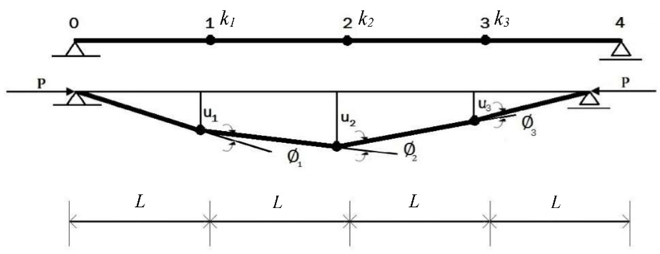
To study the complex pre- and post-buckling behaviour of a bar structure, a model in the form of straight bars with ideal hinges at the ends and subjected to axial compression force P was proposed. The bars are infinitely stiff in bending and compression, but they have elastic nodes located within the length L. This model structure provides good insight into the stability of large structural systems, because it is possible to formulate and solve problems with and without initial imperfections accounting for large displacements. A model structure was developed. It consists of four perfectly rigid bars connected by linear elastic nodes with the rotational stiffness kn, where n = 1, 2, 3 (Figure 1).
3.1. Model without Initial Geometrical Imperfections
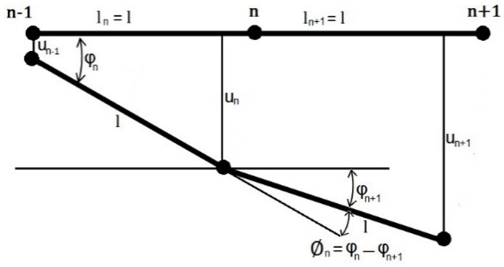
In order to determine geometrical relationships in the proposed model, a representative segment was analysed (Figure 2). Without initial geometrical imperfections, compression force P induces only elastic displacements, which are represented by superscript “e”.
Based on Figure 2, the elastic bar rotation can be expressed as follows:
The nodal rotation can be formulated in the following form:
and introducing geometrical relations (1), the following can be obtained:
where “asin” denotes arcsin.
So, the set of equilibrium equations will take the form:
For n = 1, 2, 3 the close-form Formula (4) accounting for large displacements takes the form of a set of three nonlinear algebraic equations of equilibrium:
where L = ln.
The above equations represent a non-linear eigenvalue problem, in which the elastic displacements of nodes are unknown.
In the case of small displacements, it can be assumed that , that is, the operator , then the Equation (5) becomes a linear eigenvalue problem. After the introduction of the dimensionless nodal displacement it will be received:
Equation (6) can be written in the matrix form:
where I is a unit matrix.
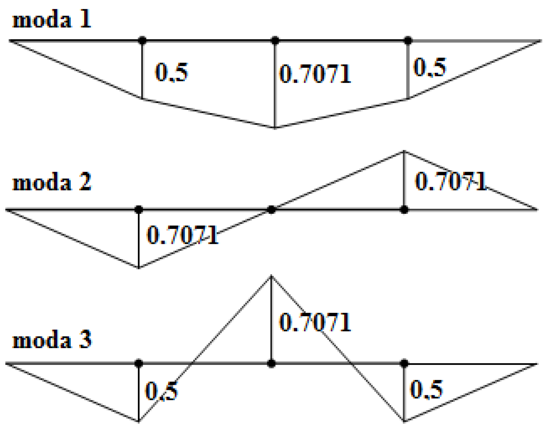
The solution of Equation (7) are the three eigenvalues (, , ) and the associated normalised eigenvectors .
The three first buckling modes obtained from the linear eigenvalue problem are presented in Figure 3.
3.2. Model with Initial Geometrical Imperfections
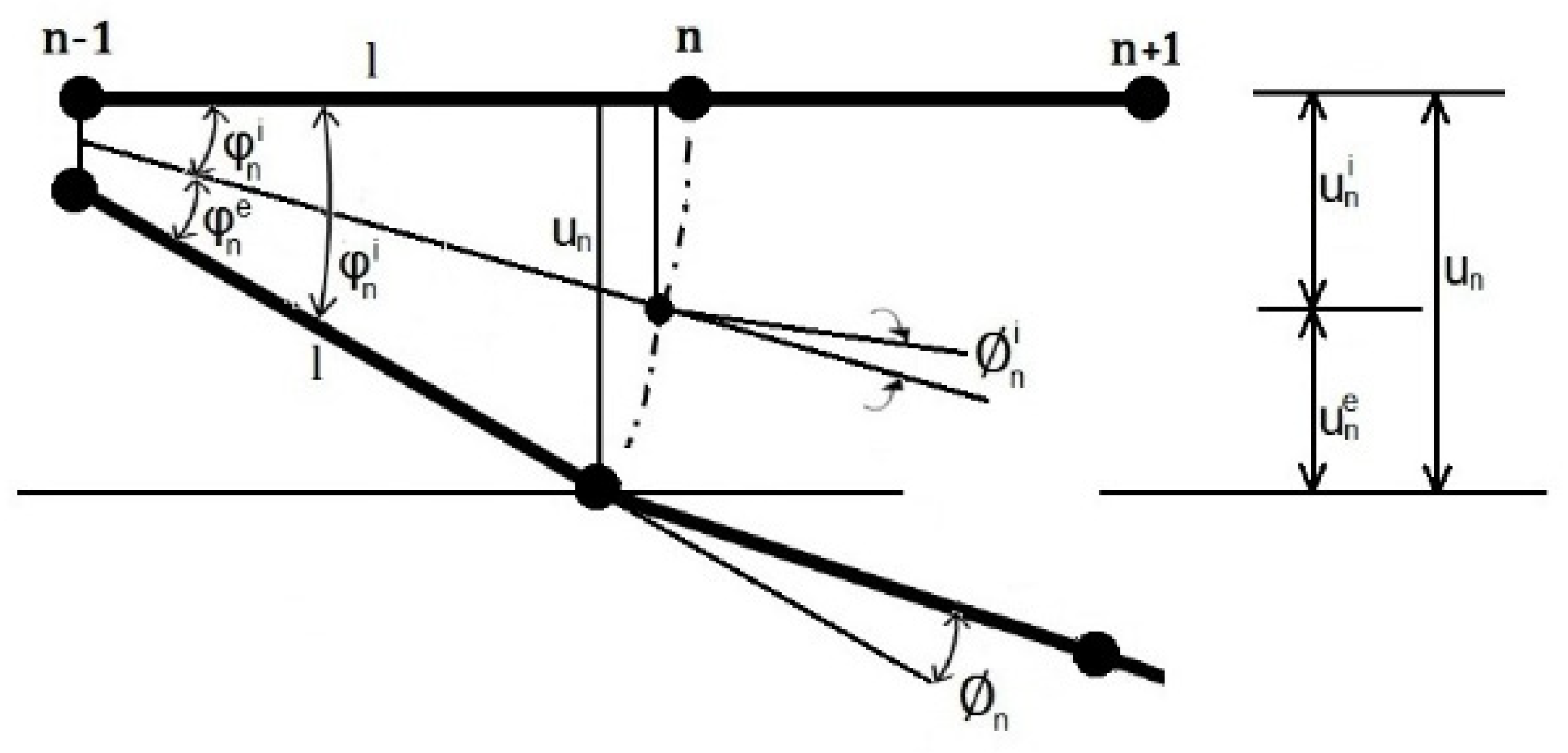
In the proposed model, initial geometrical imperfections are introduced in the form of initial nodal displacements which induce initial rotations of bars and respective node rotations (superscript “i” denote imperfections). These deformations are kinematically admissible. Therefore, they do not induce any stress. As was mentioned before, elastic deformations appear when compression force P is active. It induces moments in elastic nodes .
In order to determine geometrical relationships in the model with initial geometrical imperfections, a representative segment was analysed too (Figure 4).
Next, geometrical relations are considered in two stages. First, the initial state when compression force P is not active (P = 0), the initial bar and hinge rotations, being initial geometrical imperfections, can be described as follows:
In the second state, when compression force P is active (P > 0), displacements are the sum of the initial and elastic part and take the form:
Thus, the total hinge rotation can be expressed as:
Now, the set of non-linear equilibrium equations take the form:
For n = 1, 2, 3 the form Formula (13) takes the form of three nonlinear algebraic equations of equilibrium:
where is unknown, and is the linear combination of eigenvectors obtained as a result of the solution of a linear eigenvalue problem (7).
In order to investigate various configurations of imperfections, mode participation factors are introduced. Thus, initial node displacements can be computed as follows:
Changing the values of mode participation factor , it is possible to obtain any combination of imperfections.
4. Numerical Examples
From among many cases studied by the author, the examples shown in Figure 1 are considered. This model consists of four and three elastic nodes. In this example, the length of the bar was assumed L = 1, and compression load P = 1. Numerical examples are solved for various amplitudes of initial imperfections (Equation (15)) introduced as a linear combination of eigenvectors obtained from the linear eigenvalue problem (Equation (7)) scaled by buckling mode proportionality factor . Keeping in mind that the eigenvector is normalised, thus the displacements are not real, the buckling mode proportionality factor should be assumed so as to reflect real imperfections. This can be achieved by the measurement of imperfection in situ, based on tolerances given in codes or assumed as arbitrary amplitudes.
In this example, equilibrium paths in the model considered are analysed, taking into account different configurations of geometrical imperfections. The increasing values of imperfections associated with three successive forms of the eigenvector are considered. The amplitudes of the mode proportionality factor , used to create different configurations of the initial vector of geometrical imperfections are presented in Table 1.
Moreover, based on the analysis of potential energy, the nature of equilibrium states is described. It should be noted that the structure is in equilibrium when potential energy reaches a minimum. The necessary condition for the occurrence of minimum potential energy is the disappearance of its first variation. This condition can be written as:
In the case of the example considered, potential energy can be described according to the formula:
where λ is a load multiplier.
The nature of the equilibrium path is determined by higher order variations of potential energy. The type of bifurcation point can be determined based on the analysis of the second variation of potential energy as stable, neutral or unstable, according to:
Numerical examples are described by symbols composed of small letters of the Latin alphabet and numbers. The letter means the amplitude of the adopted buckling mode proportionality factor (m—small, s—medium, d—large), and the number—the form of a buckling mode, according to which the imperfection vector is determined, shown in Figure 3. Thus, symbol m1 denotes an example in which imperfections are introduced according to the shape of the first buckling mode with a small amplitude α1 = 0.001.
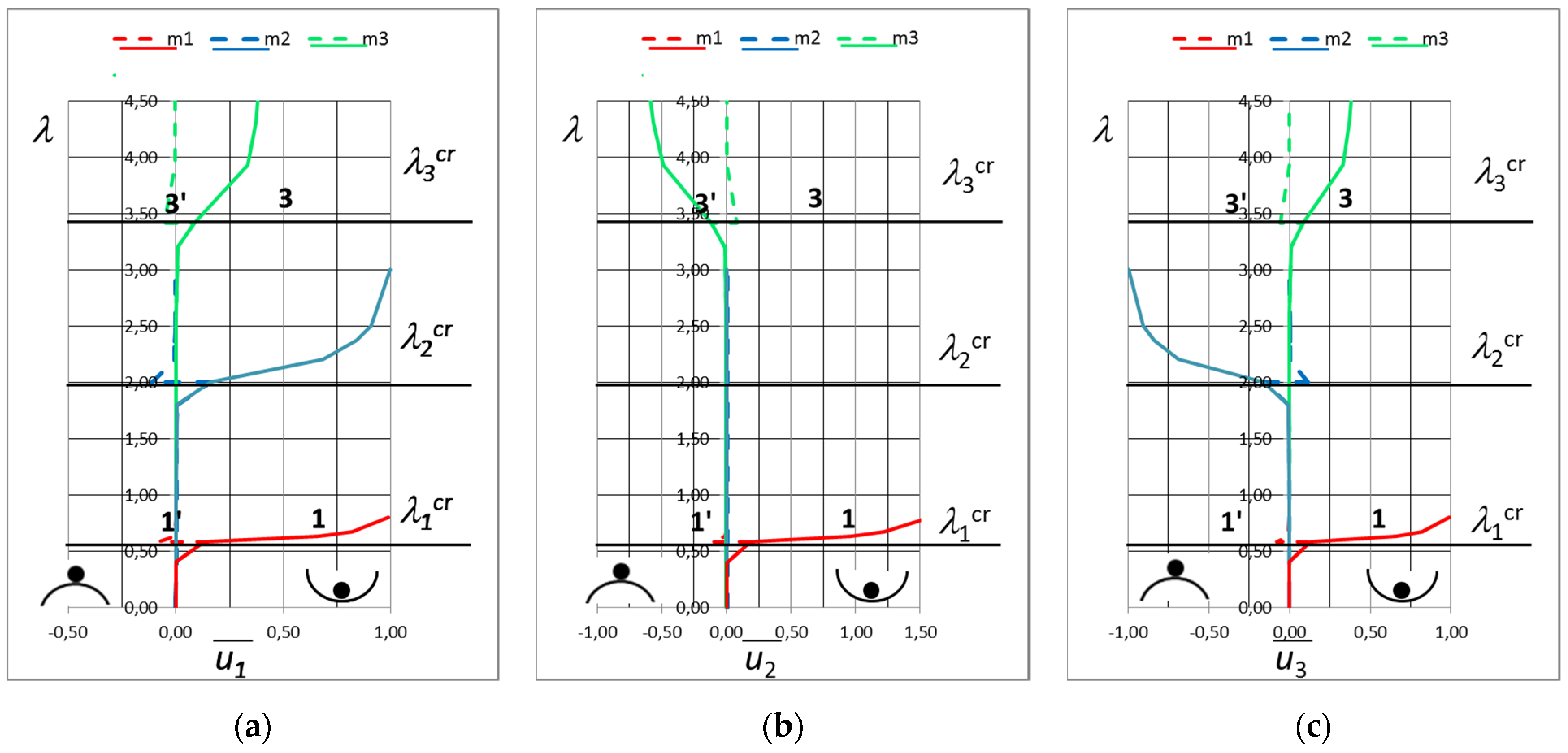
Figure 5 presents the equilibrium paths obtained for the structure with small amplitudes of initial geometrical imperfections developed in the shape of the first, second and third buckling modes, respectively (m1, m2 and m3). It is worth noting that in all three cases, a stable equilibrium path is observed, where there are points of bifurcation and the accompanying unstable equilibrium path.
When imperfection related to the first buckling, the bifurcation point corresponds almost exactly to the first eigenvalue obtained for the ideal structure. However, when imperfections are developed in accordance with the second buckling mode, the bifurcation point corresponds to the second eigenvalue, etc. It can be seen that the shape of the initial geometrical imperfection strongly determines the nature of the equilibrium path.
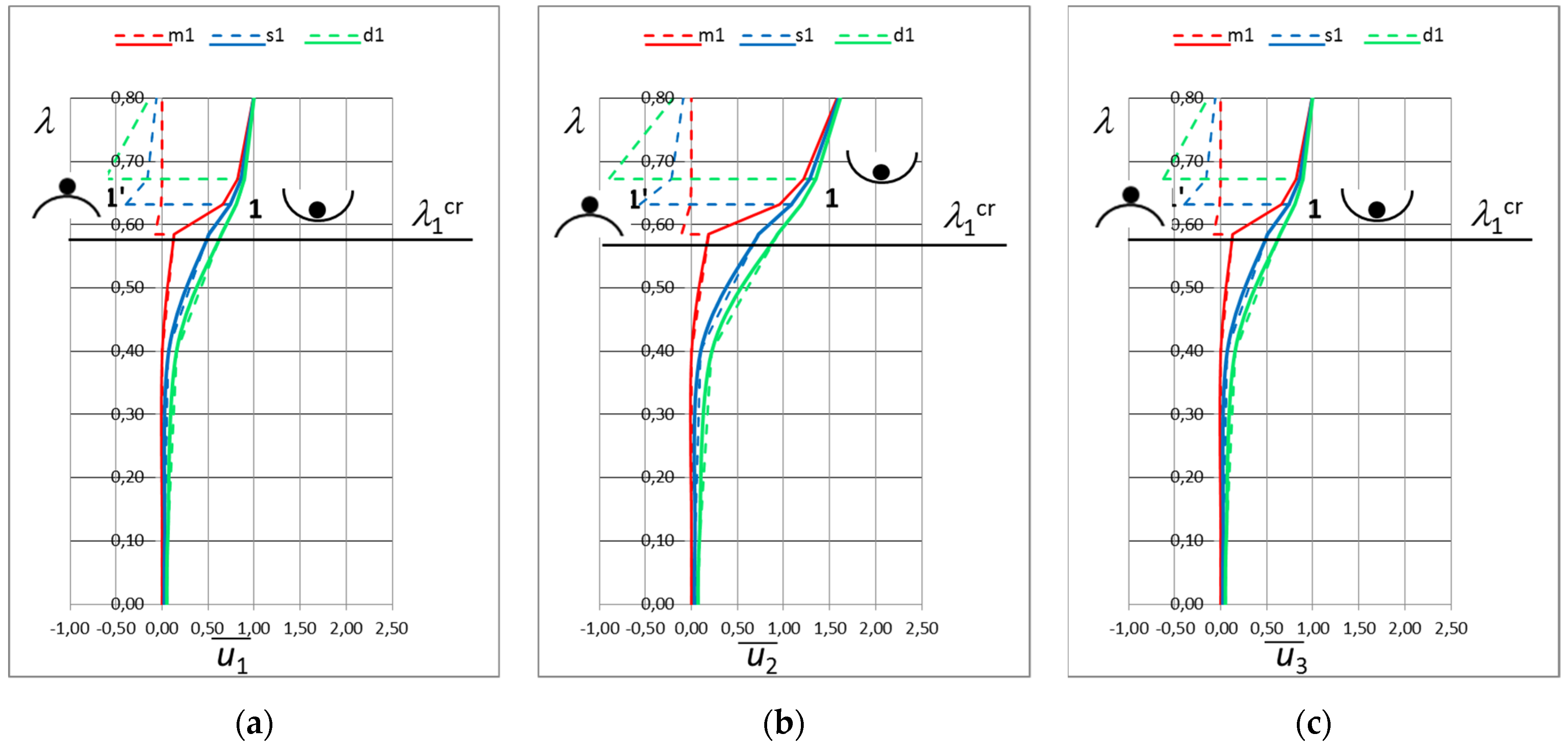
Figure 6 shows the equilibrium paths obtained for examples in which geometrical imperfections are determined according to the small, medium and large amplitude of the first buckling mode (m1, s1 and d1).
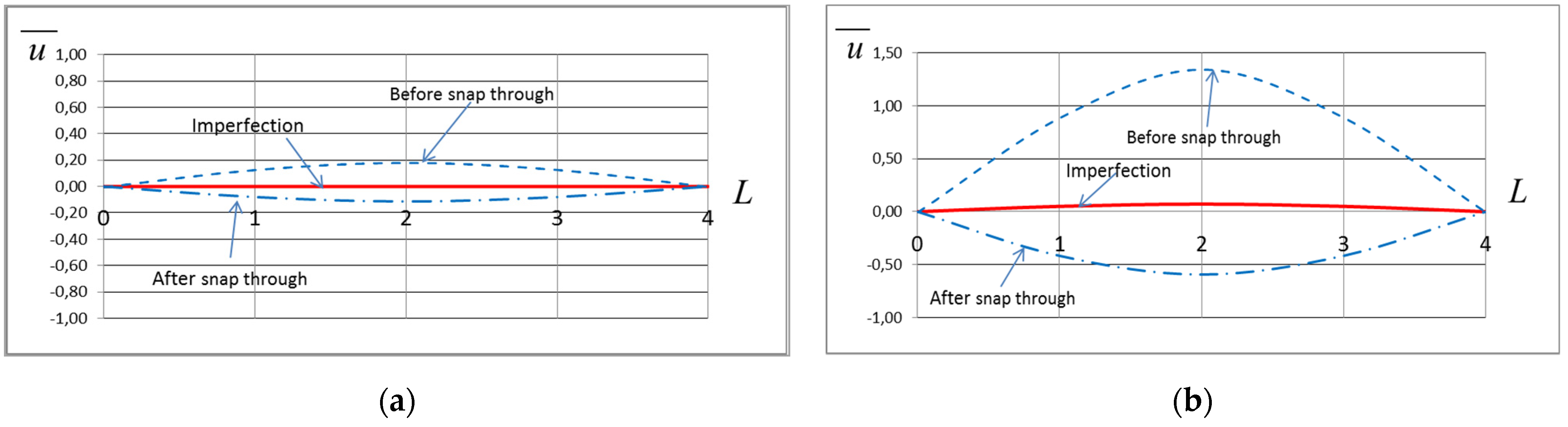
In all three cases, the bifurcation point associated only with the first critical load is observed. However, it can be observed that an increase in the amplitude of the initial geometrical imperfection results in an increase in the value of the critical load. Because the structure under consideration is primarily characterised by a stable equilibrium path, an increase in the imperfection amplitude somehow defies the snap-through of the structure to the configuration described by the unstable equilibrium path, and in this situation plays a positive role. In the case considered, the displacement both before and after the snap-through has the shape of the first buckling mode (Figure 7). Moreover, based on the analysis of the second-order variation of potential energy, it is found that before snap-through the equilibrium path is stable, and afterwards it turns into an unstable one. This is illustrated in the figures by a ball moving on a differently shaped surface.
To determine the contribution of particular buckling mode in the displacement vector for each load increment, factor is calculated according to the following relationship:
Figure 8 shows the contribution of an individual buckling mode in the displacement vector. Coefficients , and illustrate the influence of the first, second and third buckling mode on the displacement vector, respectively. It is worth noting that in the example considered, in the whole range of the equilibrium path, the first buckling mode has a significant share in the displacement vector. Thus, the initial imperfection, determined by the first buckling mode, strongly influences the shape of the total displacement vector.
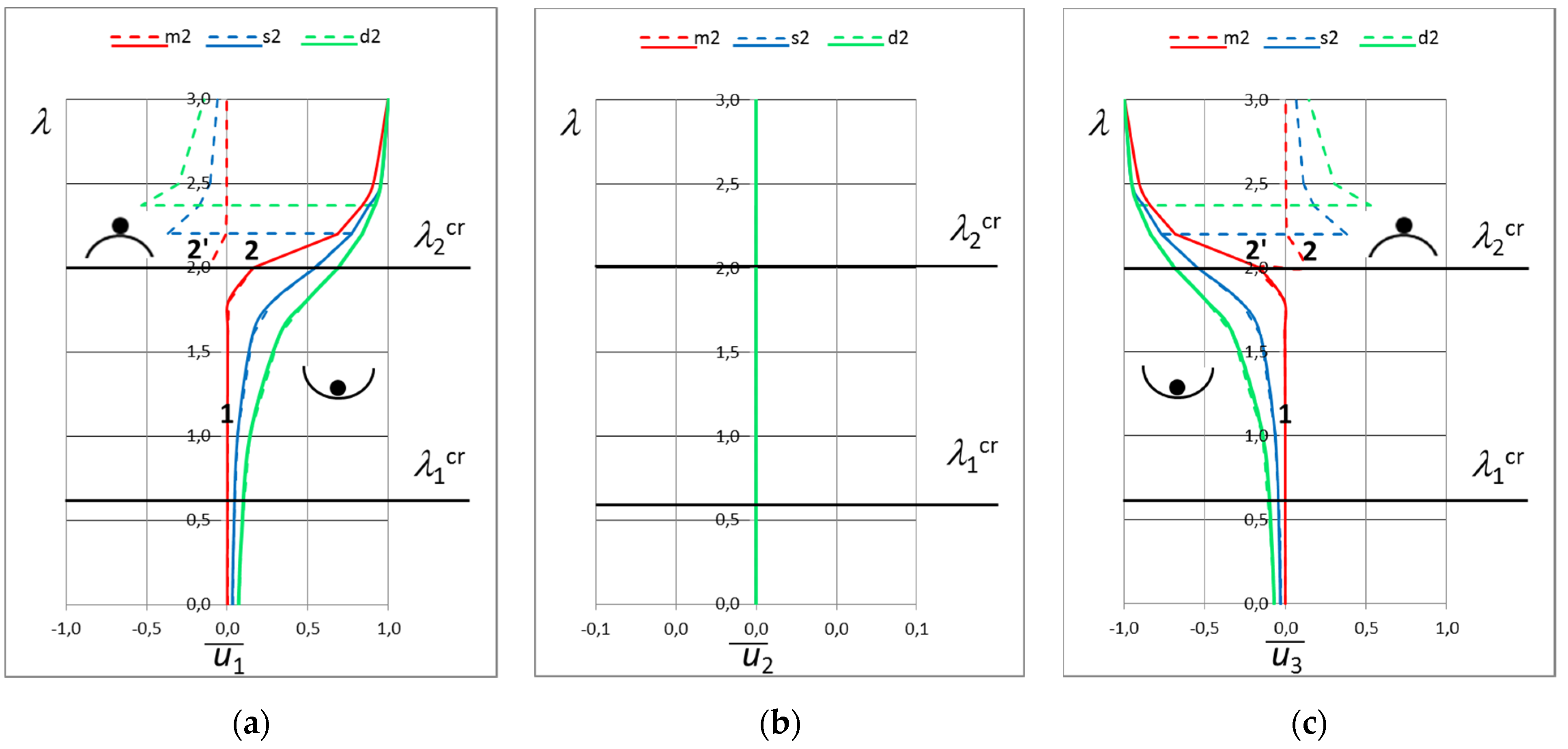
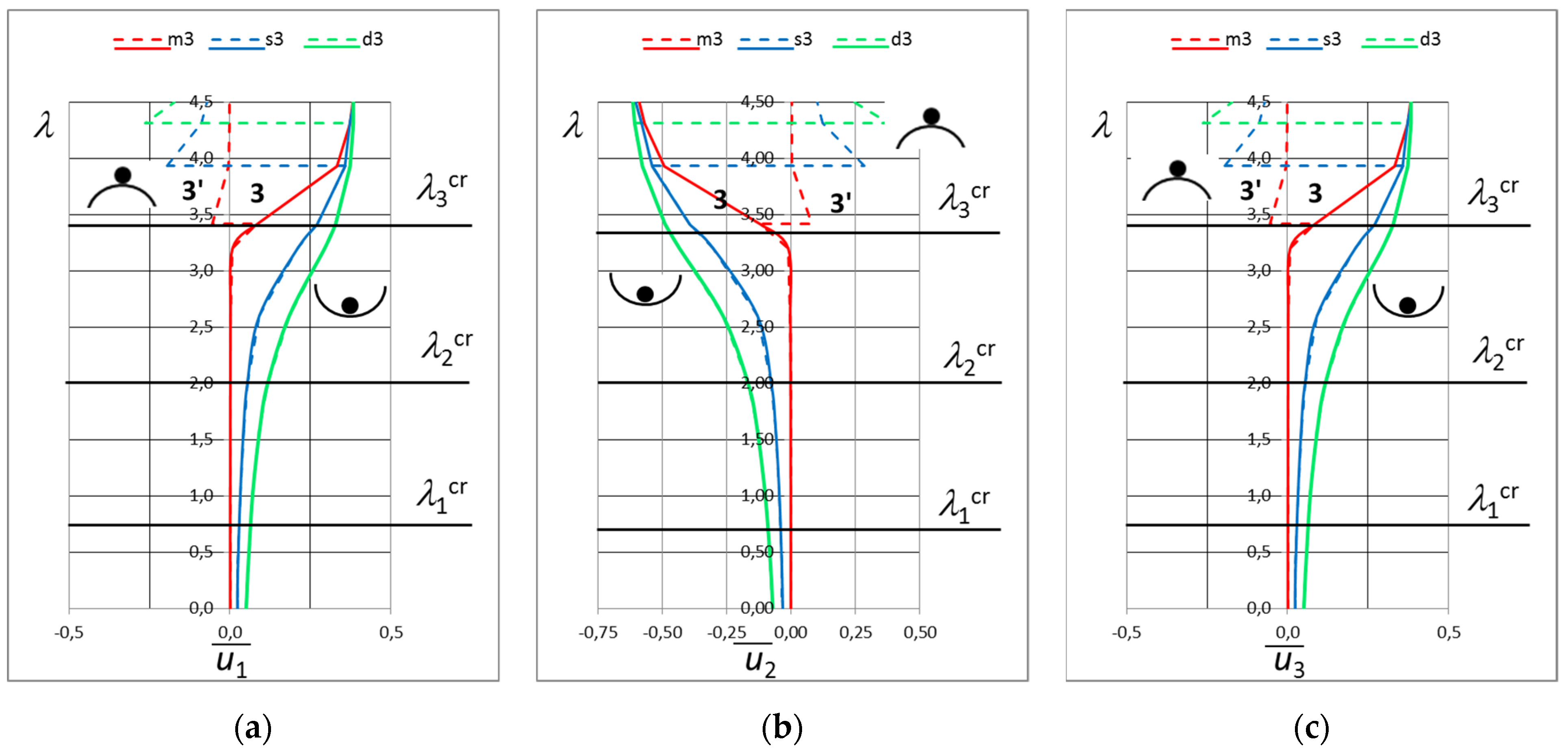
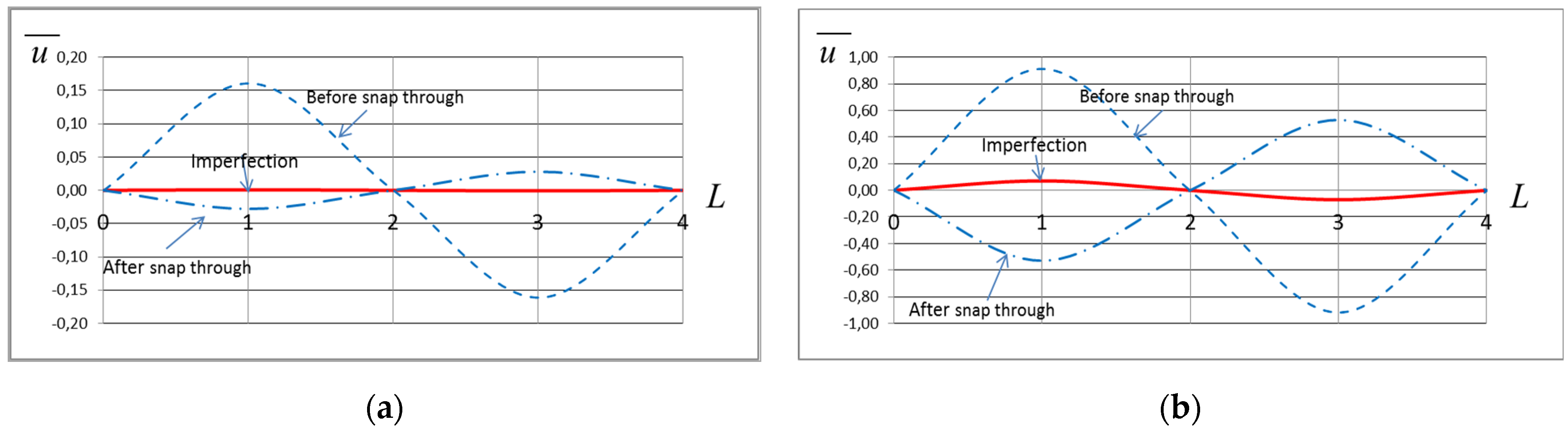
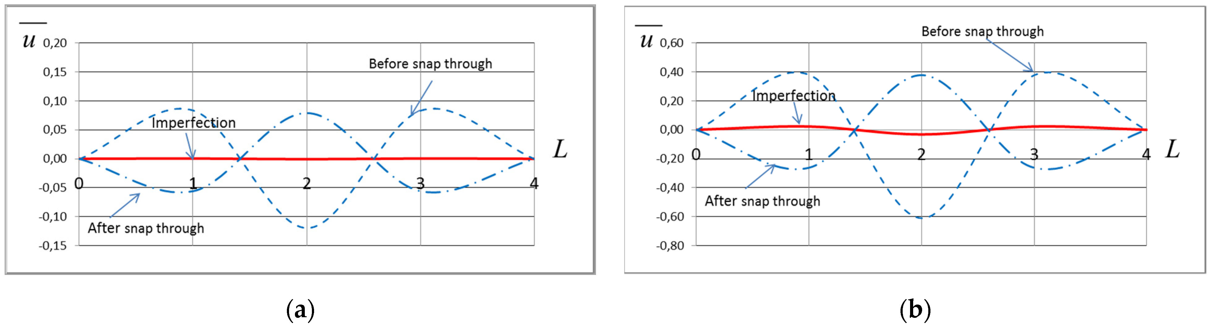
In the subsequent examples, initial geometric imperfections with three different amplitudes, developed according to the second or third buckling mode, are taken into account. For all imperfection configurations, only one bifurcation point is observed. However, the imperfection in the shape of the second buckling mode is associated with a second eigenvalue (Figure 9). In turn, for imperfections developed in accordance with the third buckling mode, the bifurcation point is associated with the third eigenvalue (Figure 10). As in the first case, an increase in the amplitude of the initial geometrical imperfection results in an increase in the value of the critical load. The displacements before and after a snap-through for all the initial amplitudes of the geometrical imperfections developed according to the second and third buckling forms have the shape of the second (Figure 11) and the third buckling form, respectively (Figure 12).
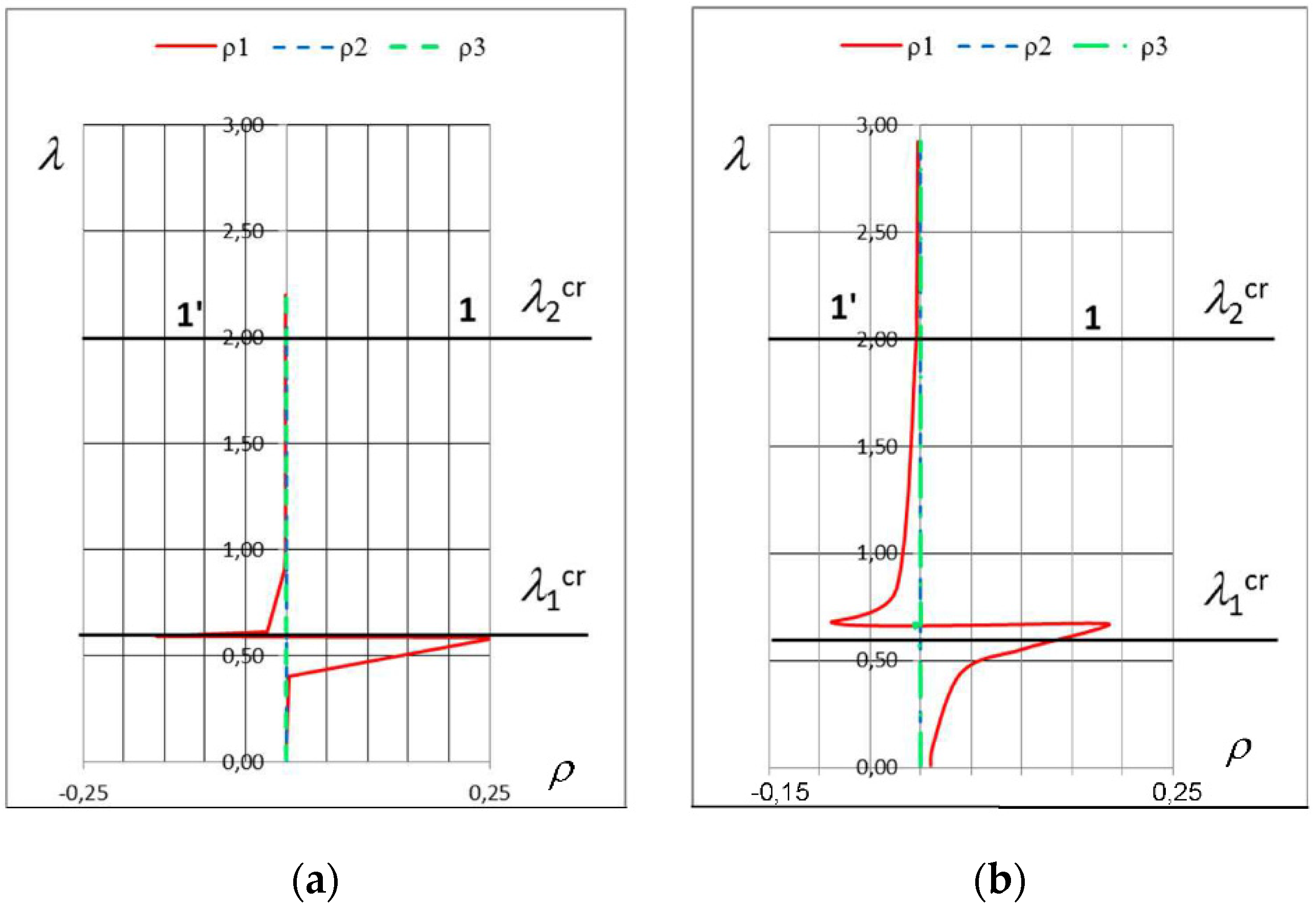
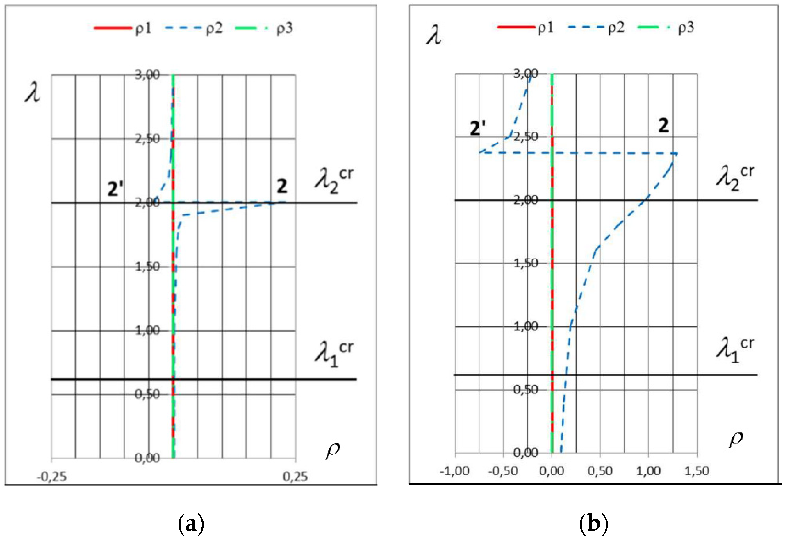
This phenomenon is confirmed by the analysis of coefficient ρ, which obtains non-zero values before and after snap-through only for the second buckling mode (Figure 13) for both small and large initial amplitudes of the geometrical imperfections developed in accordance with the second buckling mode.
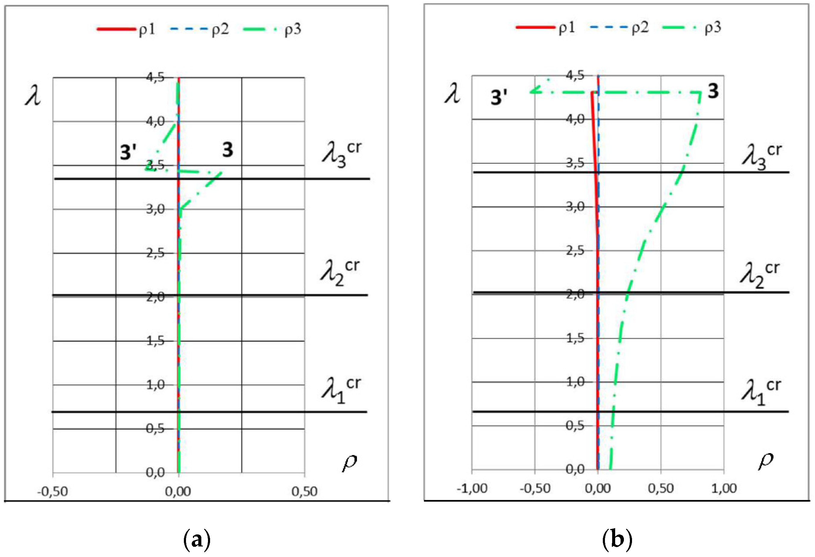
Similarly, when imperfections in the form of the third buckling mode are introduced into the structure model, non-zero values of coefficient ρ are obtained only for the third buckling mode (Figure 14).
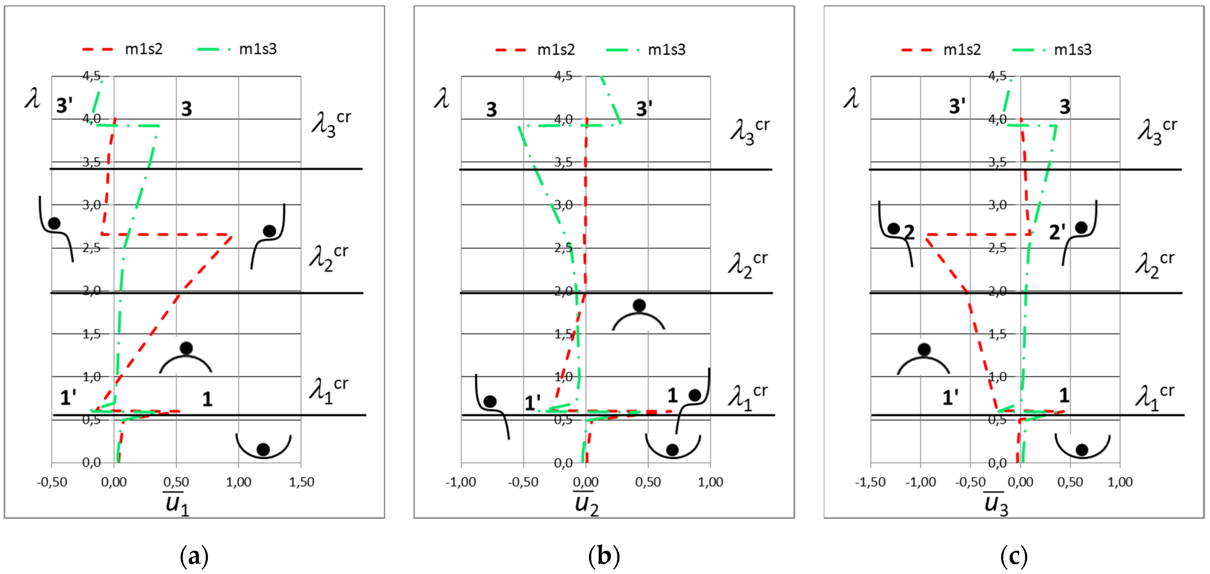
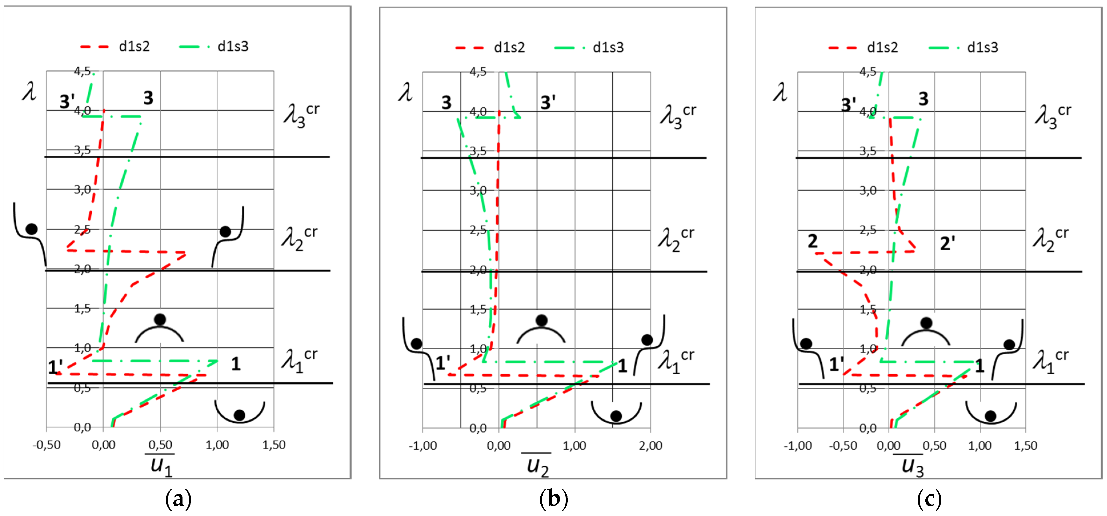
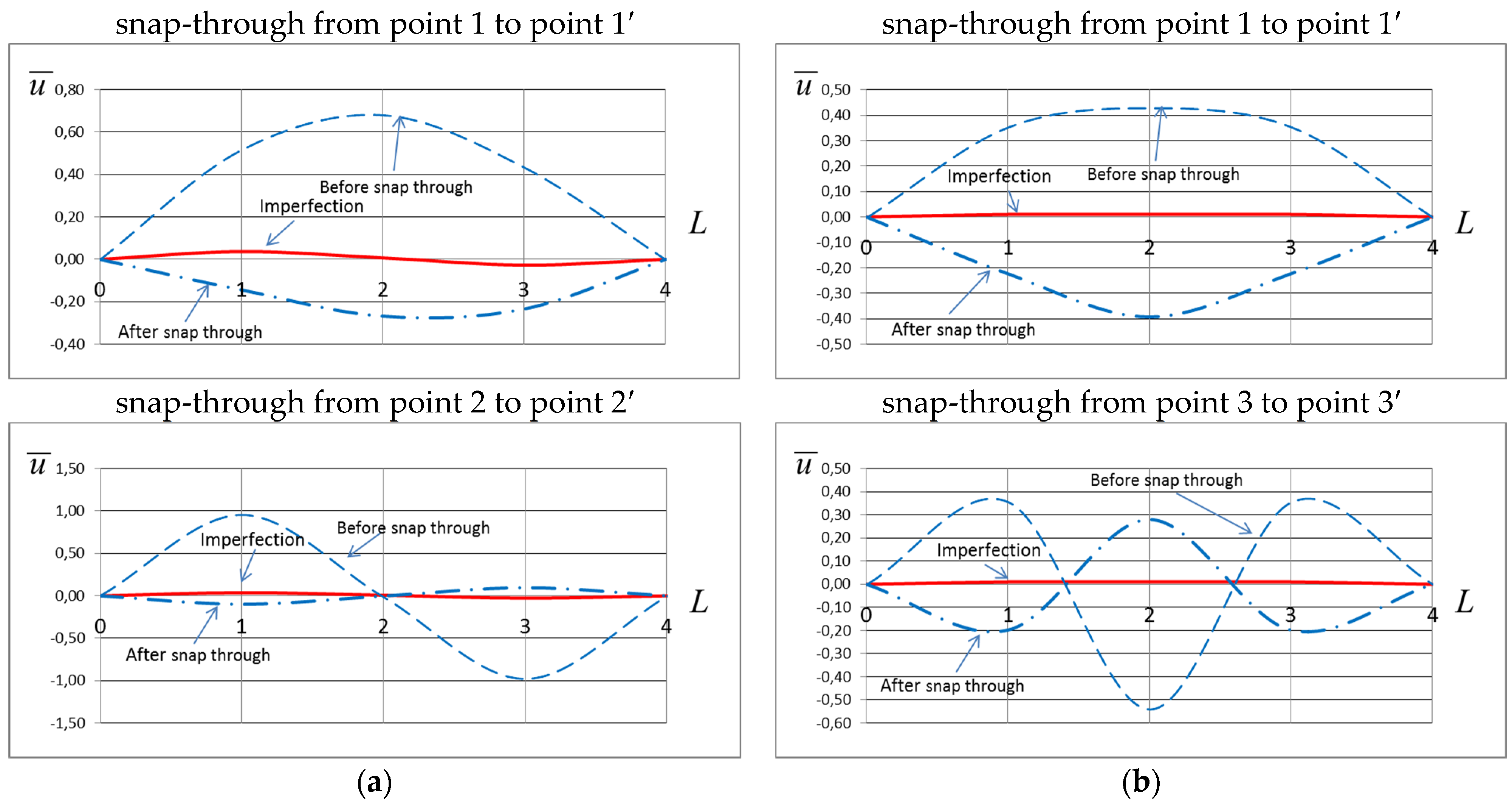
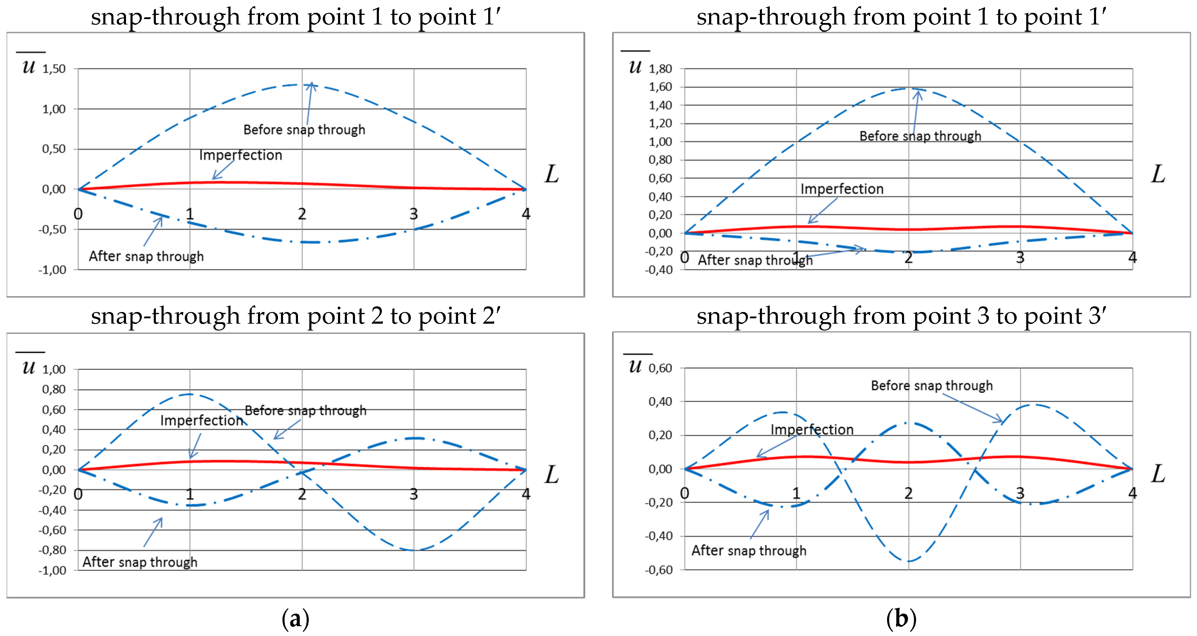
Next, analyses were carried out taking into account examples in which initial geometrical imperfections developed in the form of two different buckling modes. Figure 15 shows equilibrium paths obtained for geometrical imperfections developed according to the first low-amplitude buckling mode and second or third medium amplitude buckling mode, respectively (m1s2 or m1s3). In turn, Figure 16 shows the equilibrium paths for geometrical imperfections corresponding with a large amplitude of the first buckling mode and medium amplitude of the second or third buckling mode (d1s2 or d1s3). In all cases, two bifurcation points are observed: the first is associated with the first and the second with the second or third eigenvalue. It is observed that the introduction of geometrical imperfections developed according to two different buckling mode results in two or three snap-throughs associated with transition from the local to the global minimum of potential energy. The nature of a bifurcation point is defined by the second-order variation of potential energy and is observed to be stable before the first snap-through, and next, in case of a higher snap-through, unstable or metastable. A metastable bifurcation point is characterised by local minimum of potential energy and temporary equilibrium state. This phenomenon is illustrated by a ball moving on a differently shaped surface. The analysis of displacements before and after a snap-through shows that initial imperfection, which is a superposition of two different buckling modes, strongly influences the shape of the displacement vector.
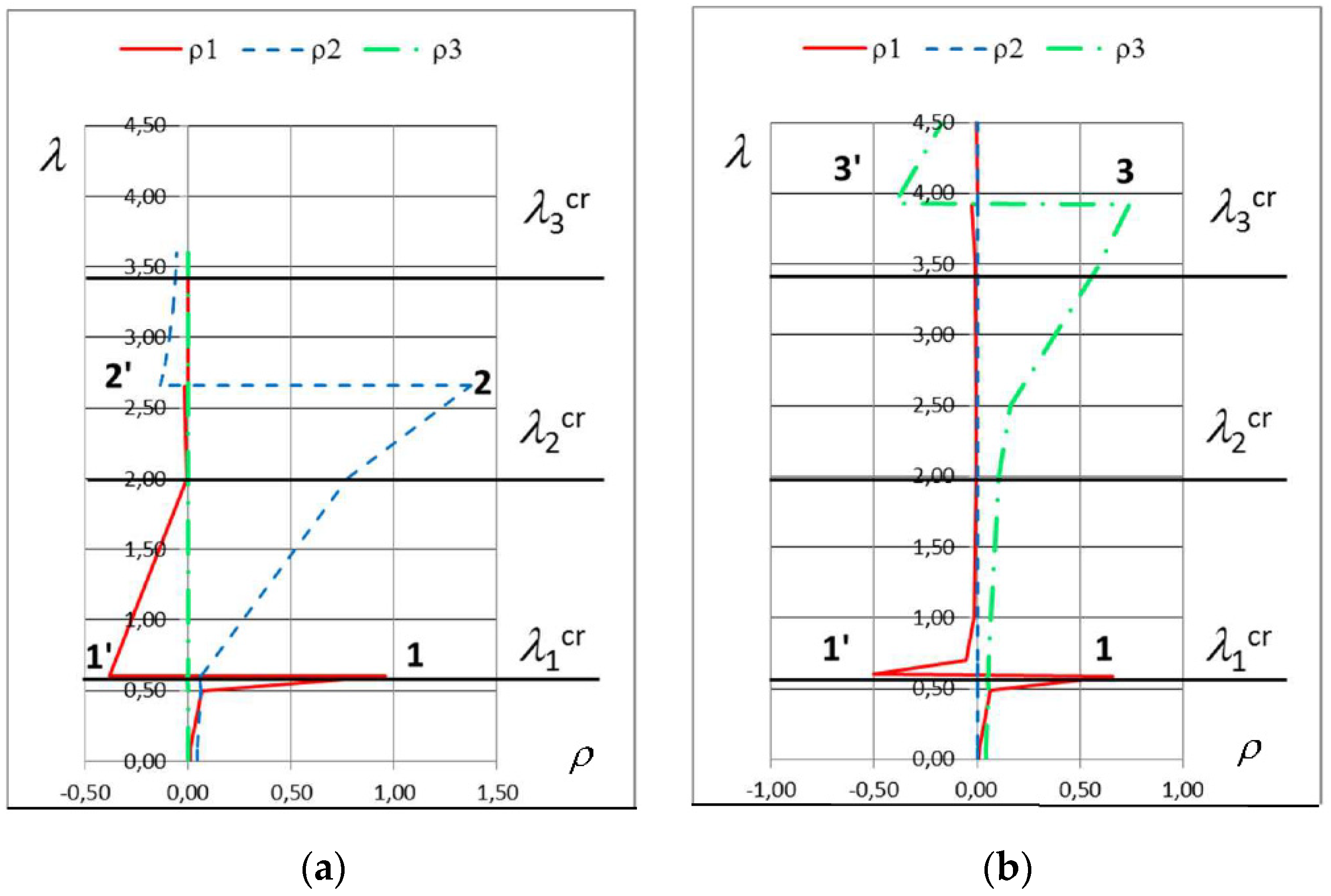
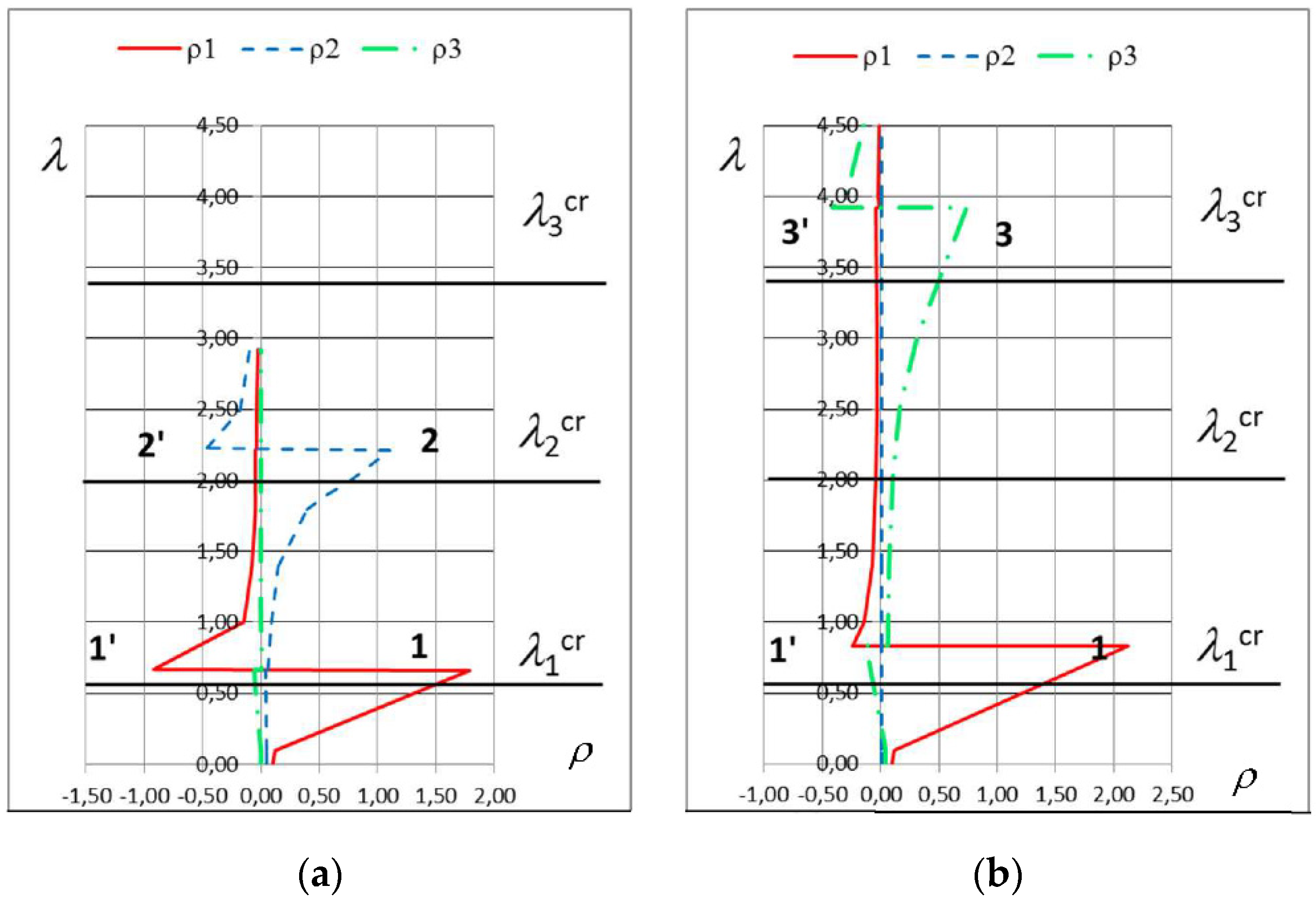
However, it is still visible that at the first bifurcation point, the most influential is the first buckling mode, at the second bifurcation point—the second buckling mode, and at third bifurcation point—the third buckling mode (Figure 17 and Figure 18). Thus, as in the previous examples, the type of initial geometrical imperfection strongly affects the whole critical path, which is also confirmed by the analysis of the coefficient of the buckling mode contribution in displacement vector ρ (Figure 19 and Figure 20). It can also be seen that in this case an increase in the amplitude of imperfection results in an increase in the value of the critical force.
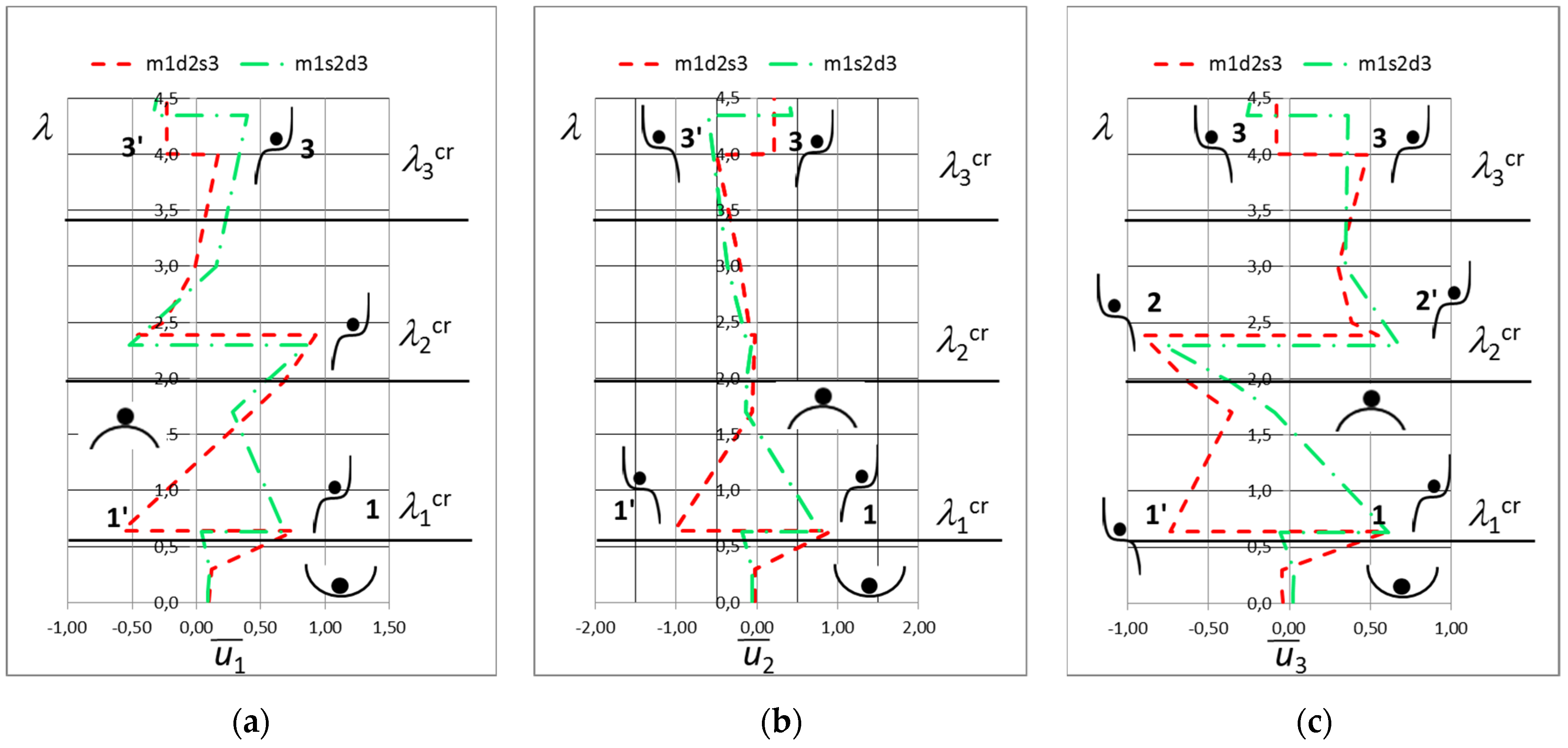
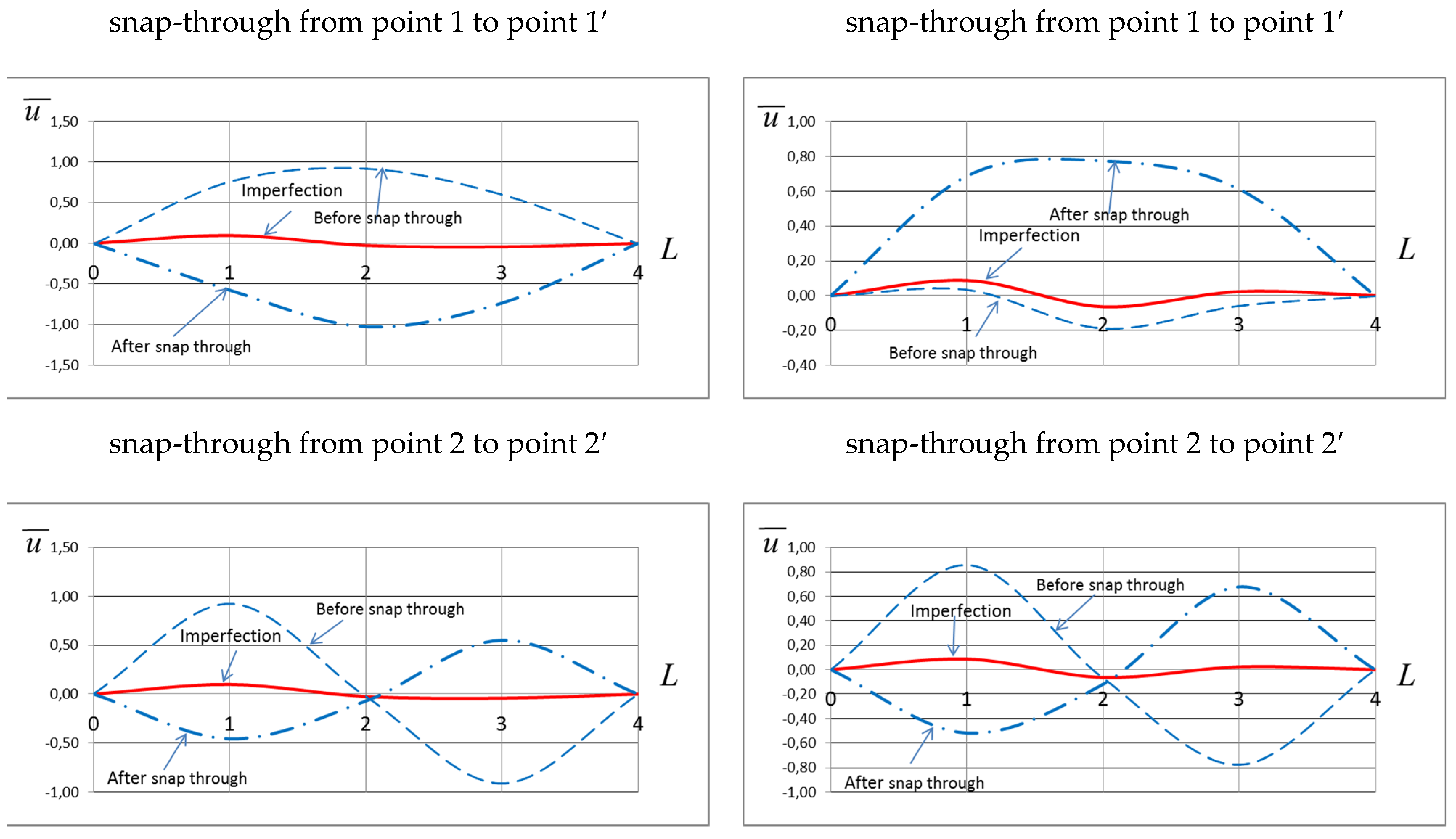
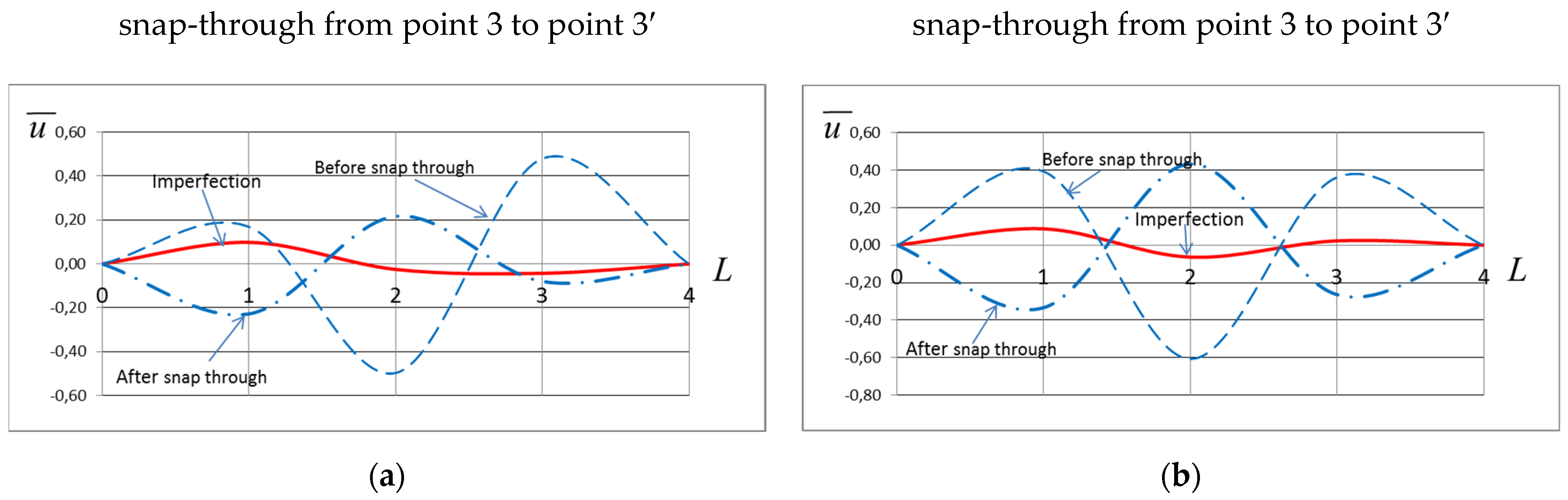
Another group are examples in which initial geometrical imperfections are developed according to three different buckling modes. In these cases, the structural response is more complicated. Figure 21 shows equilibrium paths obtained for selected configurations of initial geometrical imperfections corresponding to a small amplitude of the first buckling mode, medium or large amplitude of the second or third buckling mode m1d2s3 lub m1s2d3. In turn, in Figure 22, the pre- and post-snap through displacements observed in the above-mentioned example were compared. Three bifurcation points are observed which, depending on the type of an initial geometrical imperfection pattern, differ both in the amplitude of the displacements and the value of the eigenvalue.
It can be observed that the introduction of geometrical imperfections developed according to the three different buckling modes results in several snap-throughs which are stable, unstable or metastable. In such cases, the nature of the equilibrium path in the post-buckling range is very complex and associated with multi-transition from the local to global minimum of potential energy. Several temporary states are observed in the form of metastable bifurcation points.
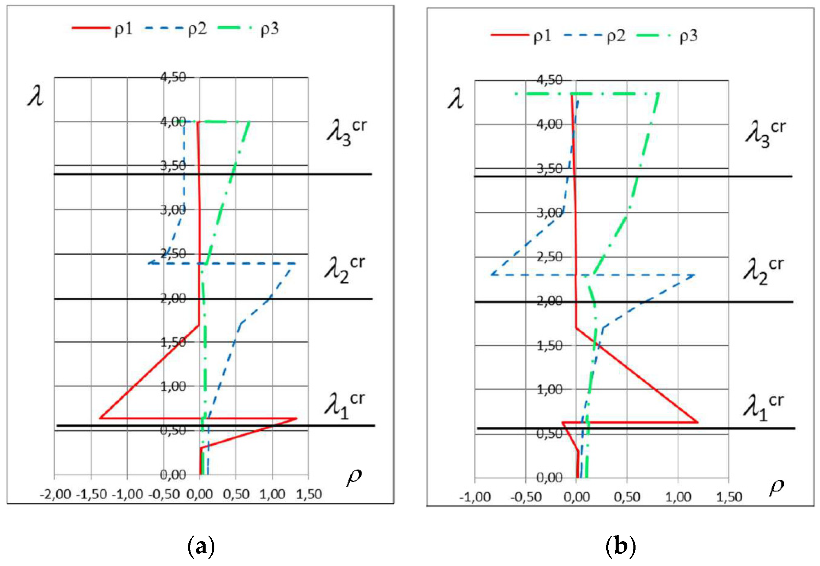
However, the snap-through is associated with the first, second, and third buckling mode, respectively. Increasing amplitudes of geometrical imperfections in the shape of the second or third form of buckling do not significantly affect the eigenvalue associated with the first buckling mode. In turn, a significant increase in the second eigenvalue is observed for a large amplitude of geometrical imperfection in the shape of the second buckling mode and, similarly, an increase in the third eigenvalue is observed for large amplitudes of imperfections developed according to the third buckling mode. The analysis of coefficient ρ leads to the conclusion that we are dealing with the interaction of three buckling modes, because in the whole range of the considered equilibrium path, all these modes are involved in the displacement vector (Figure 23). The interaction of the analysed phenomenon is also confirmed by the analysis of the deformation shape of the bar considered, before and after a snap-through. It is clearly visible that the initial geometrical imperfections, which in this case is a superposition of various amplitudes of three successive buckling modes, determine the shape of the bar displacement before and after a snap-through. There are no pure forms of deformation here that would perfectly suit subsequent buckling modes, but disrupted and asymmetrical ones. It is interesting that the maximum value of displacement before a snap-through is greater than afterwards, which indicates that the potential energy of the structure configuration changes from higher to lower.
5. Concluding Remarks
In the paper, the pre- and post-buckling behaviour of structures with various combinations of geometrical imperfections was discussed. For this purpose, nonlinear algebraic equilibrium equations were developed using the bar model. In this model, the flexibility of the beam was determined by the rotational stiffness of the nodes kn. Thus, there was possibility of tracing various forms of deformation corresponding to the buckling modes. The potentially most dangerous configurations were taken into account as a linear superposition of the three consecutive buckling modes obtained from a linear solution of the eigenvalue problem. The nature of the equilibrium states of the structure was described based on the concept of minimum of potential energy. The snap-through phenomenon based on transition from the local to the global minimum of potential energy was also detected. It was found that small amplitudes of geometrical imperfections developed in the form of the first, second or third buckling mode are accompanied by bifurcation points corresponding to the stable and unstable equilibrium paths. An increase in the amplitude of the initial geometrical imperfection results in an increase in the value of the critical load defining the bifurcation point, in which it is possible to snap through to the configuration described by unstable equilibrium paths. The observed snap-through is related to the transition of the structure from a higher to a lower level of potential energy. In this case, initial geometrical imperfections play a positive role in structural stability, forcing it to remain on a stable equilibrium path. The introduction of imperfections, developed as a linear superposition of two or three buckling modes, results in the appearance of several bifurcation points corresponding to the solution obtained for the perfect structure. In addition, in this case, an increase in the amplitude of initial geometrical imperfections results in an increase in the value of the critical force defining the bifurcation point. The analysis of the variability of the coefficient of the buckling mode contribution in displacement vector ρ showed that the initial imperfection, which is a superposition of different buckling modes, strongly influences the shape of the displacement vector, which is the effect of the interaction of buckling modes in the whole range of the equilibrium paths considered. This observation is very interesting from the engineering point of view and leads to the conclusion that in the case of a stability problem, structural engineers should be aware of real initial geometrical imperfections which can potentially cause a very dangerous failure mechanism of steel structures. It should be emphasized that the innovation of the proposed model is the ability to control imperfections and the ease of tracking multi-bifurcation post-critical equilibrium paths. Nevertheless, due to the difficulty of this issue, further theoretical and experimental research needs to be performed.
Funding
This paper was financially supported by Poznan University of Technology: 0412/SBAD/0060.
Institutional Review Board Statement
Not applicable.
Informed Consent Statement
Not applicable.
Data Availability Statement
Not applicable.
Conflicts of Interest
The author declare no conflict of interest.
References
- Timoshenko, S.P.; Gere, J.M. Theory of Elastic Stability; McGraw-Hill Book Co.: New York, NY, USA, 1961. [Google Scholar]
- EN 1993-1-1; Design of Steel Structures—Part 1-1: General Rules and Rules for Buildings. European Committee for Standardization: Brussels, Belgium, 2005.
- Vlasov, V.Z. Thin-Walled Elastic Rods; Izd-vo Akademii Nauk SSSR: Moscow, Russia, 1963. (In Russian) [Google Scholar]
- Rzeszut, K.; Garstecki, A. Modeling of initial geometrical imperfections in stability analysis of thin-walled structures. J. Theor. Appl. Mechanics. 2009, 47, 667–684. [Google Scholar]
- Dubina, D.; Ungureanu, V. Effect of imperfections on numerical simulation of instability behaviour of cold-formed steel members. Thin-Walled Struct. 2002, 40, 239–262. [Google Scholar] [CrossRef]
- Zeinoddini, V.; Schafer, B.W. Global imperfections and dimensional variations in cold-formed steel members. Int. J. Struct. Stab. Dyn. 2011, 1, 829–854. [Google Scholar] [CrossRef]
- Schafer, B.W.; Peköz, T. Computational modeling of cold-formed steel: Characterizing geometric imperfections and residual stresses. J. Constr. Steel Res. 1998, 47, 193–210. [Google Scholar] [CrossRef]
- Dubina, D.; Ungureanu, V.; Szabo, I. Codification of imperfections for advanced finite analysis of cold-formed steel members. In Proceedings of the 3rd International Conference on Thin-Walled Structures, Cracow, Poland, 5–7 June 2001; pp. 79–186. [Google Scholar]
- Kozłowski, A. Imperfekcje oraz efekty II rzędu w projektowaniu ram stalowych według PN-EN 1993-1-1. In Proceedings of the Konferencja NKILiW PAN i Komitetu Nauki PZITB, Białystok, Poland, 21–26 September 2008; pp. 311–318. [Google Scholar]
- Murzewski, J. Imperfections and P-Delta effects in multistorey steel frames. Arch. Civ. Eng. 1996, 38, 191–203. [Google Scholar]
- Barszcz, A.M.; Gizejowski, M.A. An equivalent stiffness approach for modelling the behaviour of compression members according to Eurocode 3. J. Constr. Steel Res. 2007, 63, 55–70. [Google Scholar] [CrossRef]
- Gonçalves, R. An assessment of the lateral-torsional buckling and post-buckling behaviour of steel I-section beams using a geometrically exact beam finite element. Thin-Walled Struct. 2019, 143, 106222. [Google Scholar] [CrossRef]
- Rzeszut, K.; Garstecki, A. Stability of steel structures with clearances and imperfections. In Proceedings of the VII European Congress on Computational Methods in Applied Sciences and Engineering, Crete, Greece, 5–10 June 2016; pp. 4770–4779, ISBN 978-618-82844-0-1. [Google Scholar]
- Liang, K.; Sun, Q. An accurate and efficient implementation of initial geometrical imperfections in the predictor–corrector reduced-order modeling method. Comput. Math. Appl. 2020, 79, 3429–3446. [Google Scholar] [CrossRef]
- Magisano, D.; Garcea, G. Increasing the buckling capacity with modal geometric ‘‘imperfections’’ designed by a reduced order model. Thin-Walled Struct. 2022, 178, 109529. [Google Scholar] [CrossRef]
- Cox, B.S.; Groh, R.M.J.; Avitabile, D.; Pirrera, A. Modal nudging in nonlinear elasticity: Tailoring the elastic post-buckling behaviour of engineering structures. J. Mech. Phys. Solids 2018, 116, 135–149. [Google Scholar] [CrossRef]
- Kala, Z. Computation of Equilibrium Paths in Nonlinear Finite Element Models. MATEC Web Conf. 2016, 7, 04026. [Google Scholar] [CrossRef]
- Hrinda, G.A. Snap-Through Instability Patterns in Truss Structures. In Proceedings of the Conference: 51st AIAA/ASME/ASCE/AHS/ASC Structures, Structural Dynamics, and Materials Conference 18th AIAA/ASME/AHS Adaptive Structures Conference 12th, Orlando, FL, USA, 12–15 April 2010. [Google Scholar] [CrossRef] [Green Version]
- Silva, W.T.M.; Ribeiro, K.Q. Spatial asymmetric/symmetric buckling of Mises truss with out-of-plane lateral linear spring. Int. J. Non-Linear Mech. 2021, 137, 103810. [Google Scholar] [CrossRef]
- Almuflih, A.S.; Almakayeel, N. Machine Learning-Based Model for Predicting the Shear Strength of Slender Reinforced Concrete Beams without Stirrups. Buildings 2022, 12, 1166. [Google Scholar] [CrossRef]
- Almasabha, G.; Alshboul, O.; Shehadeh, A.; Almuflih, A.S. Machine Learning Algorithm for Shear Strength Prediction of Short Links for Steel Buildings. Buildings 2022, 12, 775. [Google Scholar] [CrossRef]
- Zhao, J.; Jia, J.; He, X.; Wang, H. Post-buckling and snap-through behavior of Inclined Slender Beams. J. Appl. Mech. 2008, 75, 7. [Google Scholar] [CrossRef] [Green Version]
Figure 1.
Proposed model of the structure.

Figure 2.
Geometrical relation in the model of the structure.

Figure 3.
The buckling modes of the considered structural model.

Figure 4.
Model structure with initial imperfections.

Figure 5.
Equilibrium path obtained for small amplitudes of the geometrical imperfections in the shape of the first, second and third buckling mode, respectively (m1, m2, and m3); displacement of the node: (a) No. 1, (b) No. 2, (c) No. 3.
Figure 5.
Equilibrium path obtained for small amplitudes of the geometrical imperfections in the shape of the first, second and third buckling mode, respectively (m1, m2, and m3); displacement of the node: (a) No. 1, (b) No. 2, (c) No. 3.

Figure 6.
Equilibrium path obtained for small, medium and large amplitudes of the geometrical imperfections in the shape of the first buckling mode, respectively (m1, s1 and d1); displacement of the node: (a) No. 1, (b) No. 2, (c) No. 3.
Figure 6.
Equilibrium path obtained for small, medium and large amplitudes of the geometrical imperfections in the shape of the first buckling mode, respectively (m1, s1 and d1); displacement of the node: (a) No. 1, (b) No. 2, (c) No. 3.

Figure 7.
Configuration of displacement before and after snap-through for initial amplitudes of geometrical imperfections developed according to the first buckling mode: (a) small (m1), (b) large (d1).
Figure 7.
Configuration of displacement before and after snap-through for initial amplitudes of geometrical imperfections developed according to the first buckling mode: (a) small (m1), (b) large (d1).

Figure 8.
Coefficient ρ for geometrical imperfections developed according to the first buckling mode: (a) small (m1), (b) large (d1).
Figure 8.
Coefficient ρ for geometrical imperfections developed according to the first buckling mode: (a) small (m1), (b) large (d1).

Figure 9.
Equilibrium path obtained for small, medium and large amplitudes of the geometric imperfections in the shape of second buckling mode, respectively (m2, s2 and d2); displacement of the node: (a) No. 1, (b) No. 2, (c) No. 3.
Figure 9.
Equilibrium path obtained for small, medium and large amplitudes of the geometric imperfections in the shape of second buckling mode, respectively (m2, s2 and d2); displacement of the node: (a) No. 1, (b) No. 2, (c) No. 3.

Figure 10.
Equilibrium path obtained for small, medium and large amplitudes of the geometric imperfections in the shape of third buckling mode, respectively (m3, s3 and d3); displacement of the node: (a) No. 1, (b) No. 2, (c) No. 3.
Figure 10.
Equilibrium path obtained for small, medium and large amplitudes of the geometric imperfections in the shape of third buckling mode, respectively (m3, s3 and d3); displacement of the node: (a) No. 1, (b) No. 2, (c) No. 3.

Figure 11.
Configuration of displacement before and after snap-through for initial amplitudes of geometrical imperfections developed according to the second buckling mode: (a) small (m2), (b) large (d2).
Figure 11.
Configuration of displacement before and after snap-through for initial amplitudes of geometrical imperfections developed according to the second buckling mode: (a) small (m2), (b) large (d2).

Figure 12.
Configuration of displacement before and after snap-through for initial amplitudes of geometrical imperfections developed according to the third buckling mode: (a) small (m3), (b) large (d3).
Figure 12.
Configuration of displacement before and after snap-through for initial amplitudes of geometrical imperfections developed according to the third buckling mode: (a) small (m3), (b) large (d3).

Figure 13.
Coefficient ρ for geometrical imperfections developed according to the second buckling mode: (a) small (m2), (b) large (d2).
Figure 13.
Coefficient ρ for geometrical imperfections developed according to the second buckling mode: (a) small (m2), (b) large (d2).

Figure 14.
Coefficient ρ for geometrical imperfections developed according to the third buckling mode: (a) small (m3), (b) large (d3).
Figure 14.
Coefficient ρ for geometrical imperfections developed according to the third buckling mode: (a) small (m3), (b) large (d3).

Figure 15.
Equilibrium path obtained for geometrical imperfections in the shape of: small amplitude of the first buckling mode, medium amplitude of the second or third buckling mode, respectively (m1s2 or lub m1s3); displacement of the node: (a) No. 1, (b) No. 2, (c) No. 3.
Figure 15.
Equilibrium path obtained for geometrical imperfections in the shape of: small amplitude of the first buckling mode, medium amplitude of the second or third buckling mode, respectively (m1s2 or lub m1s3); displacement of the node: (a) No. 1, (b) No. 2, (c) No. 3.

Figure 16.
Equilibrium path obtained for geometrical imperfections in the shape of: large amplitude of the first buckling mode, medium amplitude of the second or third buckling mode, respectively (d1s2 or d1s3); displacement of the node: (a) No. 1, (b) No. 2, (c) No. 3.
Figure 16.
Equilibrium path obtained for geometrical imperfections in the shape of: large amplitude of the first buckling mode, medium amplitude of the second or third buckling mode, respectively (d1s2 or d1s3); displacement of the node: (a) No. 1, (b) No. 2, (c) No. 3.

Figure 17.
Configuration of displacement before and after snap-through for initial amplitudes of geometrical imperfections developed according to the first and second or third buckling mode; (a) m1s2, (b) m1s3.
Figure 17.
Configuration of displacement before and after snap-through for initial amplitudes of geometrical imperfections developed according to the first and second or third buckling mode; (a) m1s2, (b) m1s3.

Figure 18.
Configuration of displacement before and after snap-through for initial amplitudes of geometrical imperfections developed according to the first and second or third buckling mode; (a) d1s2, (b) d1s3.
Figure 18.
Configuration of displacement before and after snap-through for initial amplitudes of geometrical imperfections developed according to the first and second or third buckling mode; (a) d1s2, (b) d1s3.

Figure 19.
Coefficient ρ for geometrical imperfections: (a) m1s2, (b) m1s3.

Figure 20.
Coefficient ρ for geometrical imperfections: (a) d1s2, (b) d1s3.

Figure 21.
Equilibrium path obtained for geometrical imperfections in the shape of: small amplitude of the first buckling mode, medium or large amplitude of the second or third buckling mode, respectively (m1d2s3 lub m1s2d3); displacement of the node: (a) No. 1, (b) No. 2, (c) No. 3.
Figure 21.
Equilibrium path obtained for geometrical imperfections in the shape of: small amplitude of the first buckling mode, medium or large amplitude of the second or third buckling mode, respectively (m1d2s3 lub m1s2d3); displacement of the node: (a) No. 1, (b) No. 2, (c) No. 3.

Figure 22.
Configuration of displacement before and after snap-through for initial amplitudes of geometrical imperfections developed according to the first and second or third buckling mode; (a) m1d2s3, (b) m1s2d3.
Figure 22.
Configuration of displacement before and after snap-through for initial amplitudes of geometrical imperfections developed according to the first and second or third buckling mode; (a) m1d2s3, (b) m1s2d3.


Figure 23.
Coefficient ρ for geometrical imperfections: (a) m1d2s3, (b) m1s2d3.


Table 1.
Description of numerical examples.
| No. | Symbol of the Imperfection Pattern | Amplitudes of the Buckling Mode Proportionality Factor αm | ||
|---|---|---|---|---|
| α1 | α2 | α3 | ||
| 1. | m1 | 0.001 | 0 | 0 |
| 2. | m2 | 0 | 0.001 | 0 |
| 3. | m3 | 0 | 0 | 0.001 |
| 4. | s1 | 0.045 | - | - |
| 5. | s2 | - | 0.045 | - |
| 6. | s3 | - | - | 0.045 |
| 7. | d1 | 0.1 | - | - |
| 8. | d2 | - | 0.1 | - |
| 9. | d3 | - | - | 0.1 |
| 10. | m1s2 | 0.001 | 0.045 | - |
| 11. | m1s3 | 0.001 | - | 0.045 |
| 12. | d1s2 | 0.045 | 0.1 | |
| 13. | d1s3 | 0.1 | - | 0.045 |
| 14. | m1d2s3 | 0.001 | 0.1 | 0.045 |
| 15. | m1s2d3 | 0.001 | 0.045 | 0.1 |
Publisher’s Note: MDPI stays neutral with regard to jurisdictional claims in published maps and institutional affiliations. |
© 2022 by the author. Licensee MDPI, Basel, Switzerland. This article is an open access article distributed under the terms and conditions of the Creative Commons Attribution (CC BY) license (https://creativecommons.org/licenses/by/4.0/).
Share and Cite
MDPI and ACS Style
Rzeszut, K. Post-Buckling Behaviour of Steel Structures with Different Types of Imperfections. Appl. Sci. 2022, 12, 9018. https://doi.org/10.3390/app12189018
AMA Style
Rzeszut K. Post-Buckling Behaviour of Steel Structures with Different Types of Imperfections. Applied Sciences. 2022; 12(18):9018. https://doi.org/10.3390/app12189018
Chicago/Turabian StyleRzeszut, Katarzyna. 2022. "Post-Buckling Behaviour of Steel Structures with Different Types of Imperfections" Applied Sciences 12, no. 18: 9018. https://doi.org/10.3390/app12189018
Note that from the first issue of 2016, this journal uses article numbers instead of page numbers. See further details here.