1. Introduction
Climate models predict continued global warming in the future [
1]. This phenomenon affects all areas of people’s lives. With the development of the tourism industry, the Monorail Tour Transit System (MTTS) has been increasingly applied and promoted. The entire route of the monorail tourism system is elevated, and consists of foundations, steel columns, supports, beam-column nodes, steel track beams, and rail-holding trains [
2]. Under the direct influence of climate change, the nonlinear temperature gradient generated by some structures will cause nonlinear section deformation, resulting in self-equilibrium stress [
3,
4,
5,
6,
7,
8]. Temperature is an essential factor affecting the structural design and damage, and the temperature field of steel beams’ structure is changed over time by environmental factors. The track beam of a monorail tourism system is exposed to factors in the external environment, such as the atmospheric temperature and solar radiation, for a long time. The solar temperature field produces a nonlinear temperature distribution (i.e., gradient temperature load) inside the structure, which has a large impact on its internal strength and linearity. The corresponding temperature stress and deformation are important elements that should be considered in the structural design. Deformation has a great impact on the running safety and the running comfort of the monorail train travel system. In severe cases, it may cause disease or even damage to the beam-column joints. Relevant studies have shown that seasonal temperature differences can cause a maximum axial stress change of 20 MPa in some types of structures, such as long-span steel-mesh domes [
9]. Therefore, it is necessary to conduct in-depth research on the distribution of the temperature field of sunlight in unpaved steel beams in monorail tourism systems, and to derive a temperature-gradient model suitable for pure steel beams, which can be used as a reference for engineering design and a useful supplement to relevant industry codes and standards.
Many scholars have recently researched the sunshine’s temperature field in concrete box girders and steel box girders. Liu et al. [
10] proposed a monitoring scheme and established a thermal field model for steel box girders. Through field monitoring and numerical simulation of the Tongling Yangtze River Bridge (TL Bridge), they studied the thermal-field characteristics of the steel bridge deck, when the asphalt pavement was paved. Sallal R. Abid et al. [
11] recorded experimental data on the test beam section for six months in hot and cold seasons using actual measurements, and discussed the influence of air temperature and solar radiation on the distribution of the temperature gradient in concrete-wrapped composite beams (I-shaped beams). Wang et al. [
12] analyzed the thermal stress response and variation trend of simple temperature and continuous constrained boundary conditions under different temperature loads through an experimental study on the effect of a 1:4 ratio temperature gradient. Xu et al. [
13] studied the law of variation of the temperature field in the long-span cable-stayed bridge, based on the monitoring data of the temperature of the Nanjing Third Yangtze River Bridge. They used the generalized Pareto model to predict the extreme temperature value of the 100-year return period. Sallal R. Abid et al. [
14,
15] studied the thermal response of the standard steel section itself under different geometric parameters, based on a measured test of the steel components combined with a finite element thermal analysis. Wang et al. [
16] conducted temperature tests on two steel structure specimens with different cross-sections under open-air sunshine conditions, and then summarized and analyzed the laws of temperature variation in the components. However, the object of this study is the unpaved steel box girder, which is characterized by no pavement and a narrow beam width. There are two problems in the current research: one is that there is no corresponding design code in China, and the other is that some design codes do not apply to this research object. There are few studies on the sunshine temperature field and gradient temperature load of steel beams without pavement, and the relevant regulations are not suitable for designing steel beams without pavement. Therefore, considering the safety and economy of the structure, it is necessary to study the temperature field of steel beams without pavement.
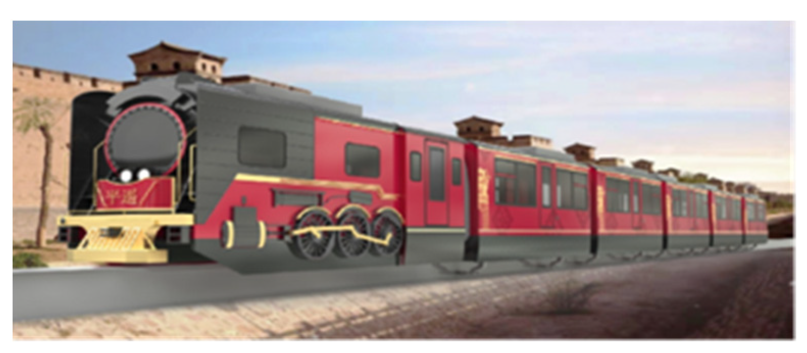
In this paper, taking the Shanxi Pingyao tourist train project, as shown in
Figure 1, as the engineering background, the temperature field of the steel track beam without pavement is studied using the field measurement method. The temperature gradient distribution characteristics and variation law of the steel box girder without pavement are analyzed; the curve form of the temperature gradient is determined by standard comparison; finally, the generalized extreme value distribution model is used to analyze the temperature difference between the 50-year return period and the 100-year return period. The representative values are predicted, and the temperature base values for different return periods and the complete temperature gradient model are determined.
2. Experimental Work
The track beam structure mostly consists of slender members running in the longitudinal direction. Studies have shown that the temperature distribution along the longitudinal direction of the bridge can be assumed to be uniform (that is, the heat flow along the longitudinal direction of the bridge can be ignored). Therefore, the unit-length track beam segments of typical cross-sections are studied here.
Figure 2a shows the test steel beam, while
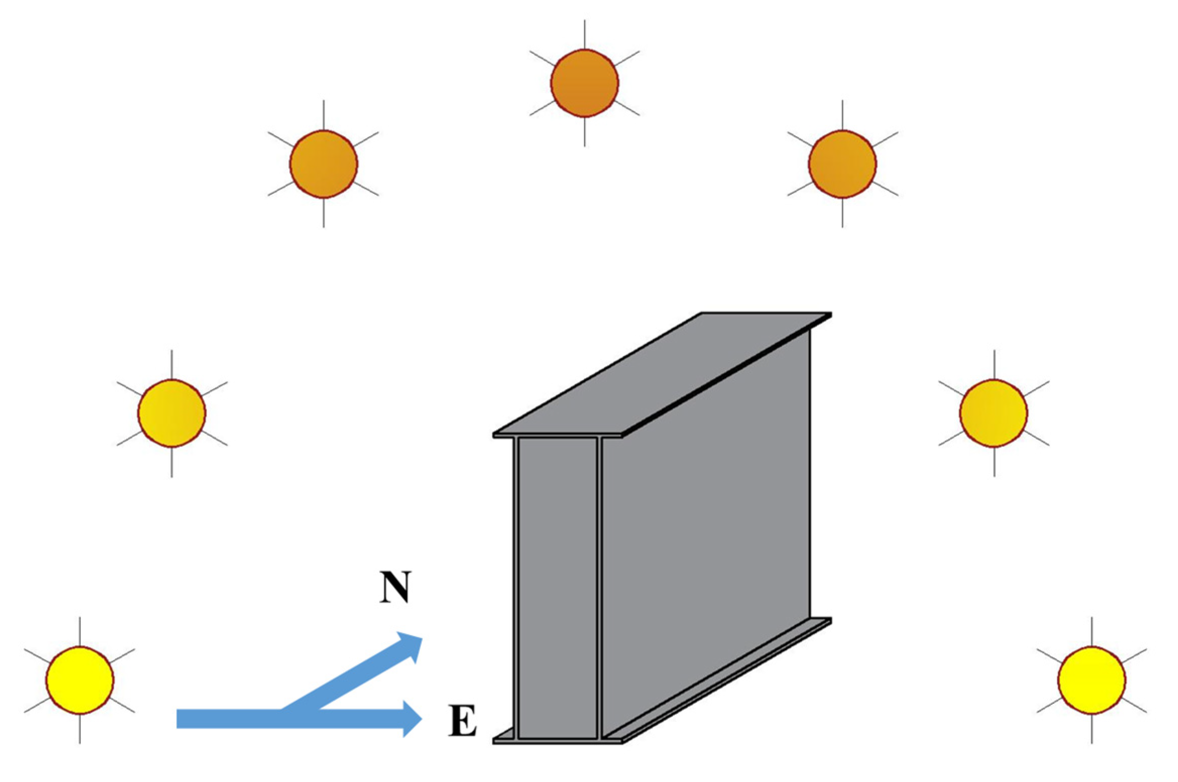
Figure 2b shows the specimen section’s geometric dimension diagram and the sensors’ positions. As shown in the figure, the test piece was welded with Q345 steel with a thickness of 6 mm, and the surface was painted gray. The sensor is a PT100 platinum resistance temperature sensor (accuracy ±0.15 °C, temperature measurement range −60~200 °C), and the acquisition module is the JY-DAM-PTX series temperature acquisition module (temperature measurement accuracy ±0.1 °C, acquisition frequency 10 Hz). The orientation and surface orientation of the track beam structure have a significant impact on the temperature distribution of the web, and the distribution of the maximum temperature difference along the thickness of the web [
17]. For the most unfavorable situation, the length of the specimen was placed in an open area (latitude 37.2 °N) along the north–south direction to meet the requirements of the maximum sunlight exposure during the day, as shown in
Figure 3. To account for the influence of the surface of the steel beam, the air convection heat exchange, and solar radiation reflection, the beam segment was placed on brick, and the bottom plate was not in contact with the ground.
3. Experimental Results
The testing period was from 31 January 2021 to 22 March 2022. Under normal circumstances, the specific heat of steel is 0.48 × 10³ J/(kg·°C), and the thermal conductivity is 48 W/(m·K). The specific heat of air in the environment is 1.0 × 10³ J/(kg·°C), and the thermal conductivity is 0.023 W/(m·K). Therefore, under the same conditions, the steel temperature rises faster than the ambient temperature when the same amount of heat is absorbed. After screening a large amount of data, we selected representative periods of July 2021 (summer) and December 2021 (winter), i.e., two months of data, for analysis.
3.1. Diurnal Variation of Temperature at the Measuring Point
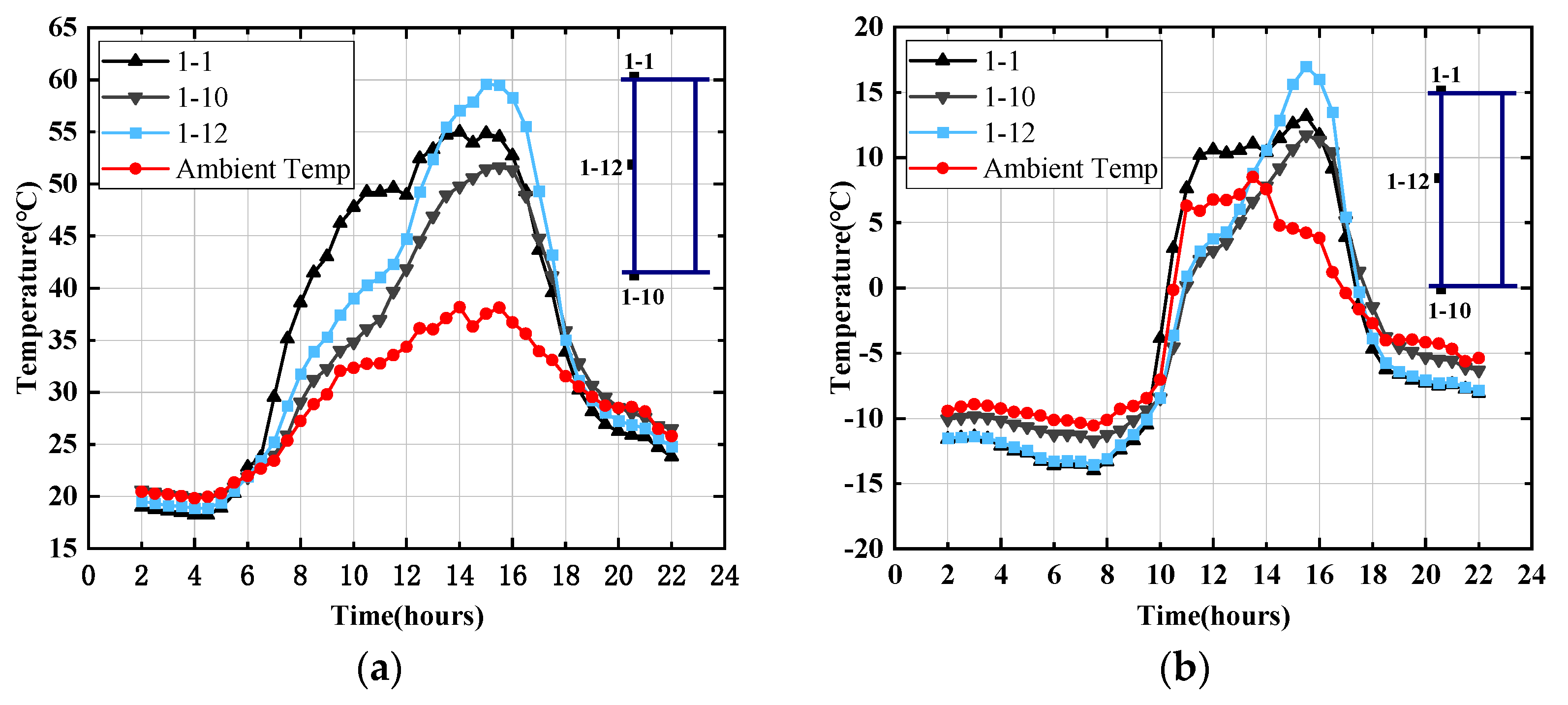
This section analyzes the diurnal variation behavior of the temperature at the measuring point identified, based on the monitoring data on 30 July 2021 and 26 December 2021. The frequency of the data monitoring is 1 min, and the average value is taken every 30 min. It can be seen from
Figure 4 that the daily temperature variation behaviors at 1-1, 1-10, and 1-12 are basically the same, but there is an apparent time-lag compared with the ambient temperature (considering the solar radiation). In summer, the days are long and the nights are short. As shown in
Figure 4a, starting at 5:00 in the morning, the roof surface is the first to receive solar radiation, and the 1-1 temperature starts to rise first in the environment. Then, 1-12 and 1-10 are located in the middle of the web and the bottom of the specimen, respectively, and their temperature rise lags behind that of 1-1. In addition, 1-12 has a larger beam angle and a longer duration of solar radiation than other measuring points, so the maximum temperature of 1-12 was greater than that of 1-1 and 1-10. After sunset, the temperature of the measuring point dropped and the lowest temperature at 1-1, 1-12, and 1-10 appeared around 4:30 in the morning, and the size was basically the same.
In winter, the day is short and the night is long, so the exposure time of the specimen is shorter than that in summer. The temperature changes in 1-1, 1-12, and 1-10 shown in
Figure 4b lag behind the ambient temperature changes. From 9:00 a.m. to 18:00, the duration of significant changes in temperature in the structure is about 3 h less than in summer. The lowest temperature of the structure occurred at the 1-1 position around 5:00 in the morning. The temperature change in the nighttime structure was gentle in both summer and winter.
3.2. Monthly Variation of Daily Maximum Temperature at Measuring Point
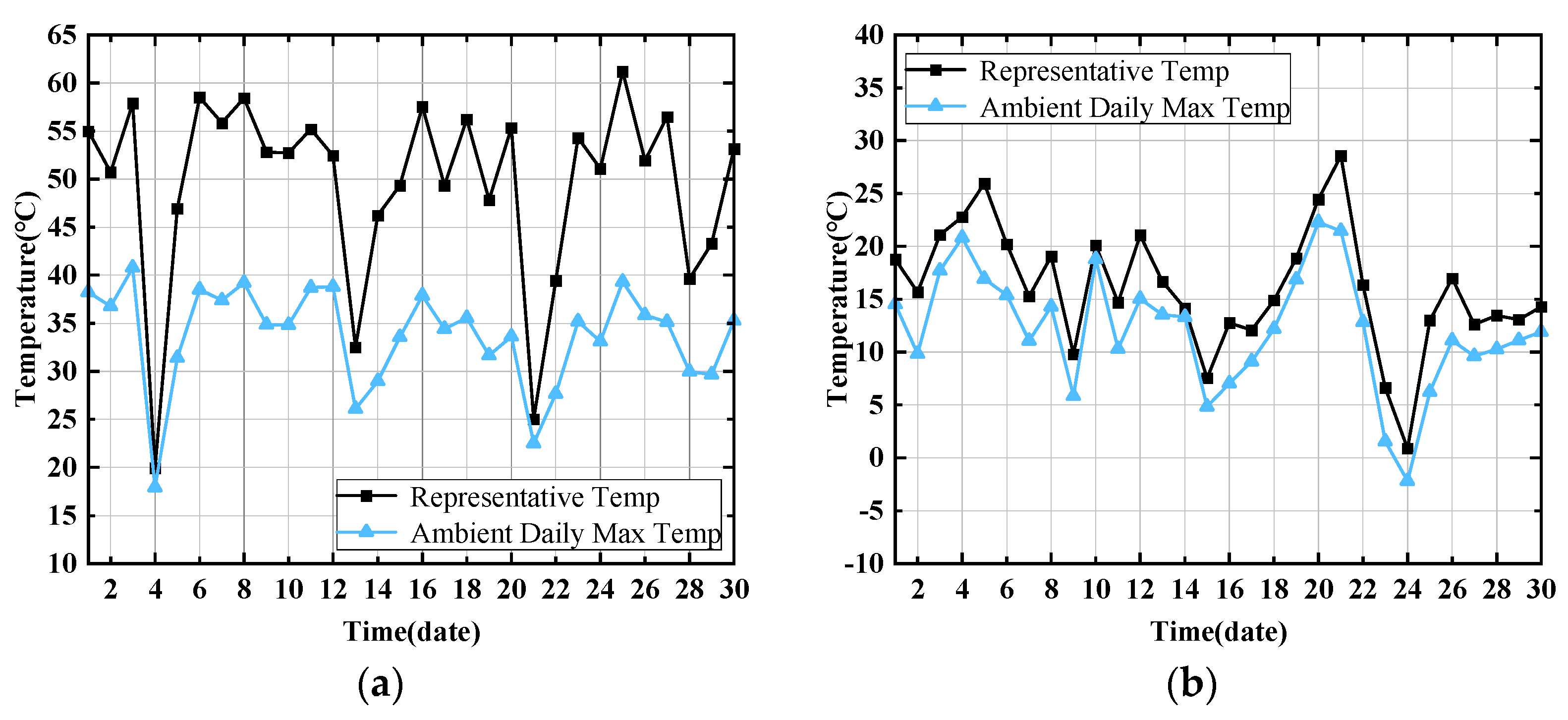
We selected the highest temperature of the day among all the measuring points as the representative temperature of the component. When the influence of solar radiation is considered, this component’s representative temperature correlates strongly with the maximum ambient temperature of the day. The temperature rise and temperature drop of this component’s representative temperature and the daily maximum temperature of the environment are basically the same, and their trends of change are the same. Furthermore, the temperature change is generally more affected by the environmental temperature change than by the solar radiation and wind speed.
As shown in
Figure 5, during the summer, from 3 July to 5 July and from 20 July to 21 July, the maximum daily temperature of the environment changed significantly, and the representative temperature of the component also showed a significant change in the same direction. During the summer, from 11 July to 12 July, and the winter, from 16 December to 17 December and from 28 December to 29 December, the wind speed was analyzed as a sensitive factor affecting the convection coefficient on the component’s surface. Therefore, while the maximum temperature of the ambient day increased slightly, the representative temperature of the component decreased slightly, and the changing trend of the two was relatively inconsistent.
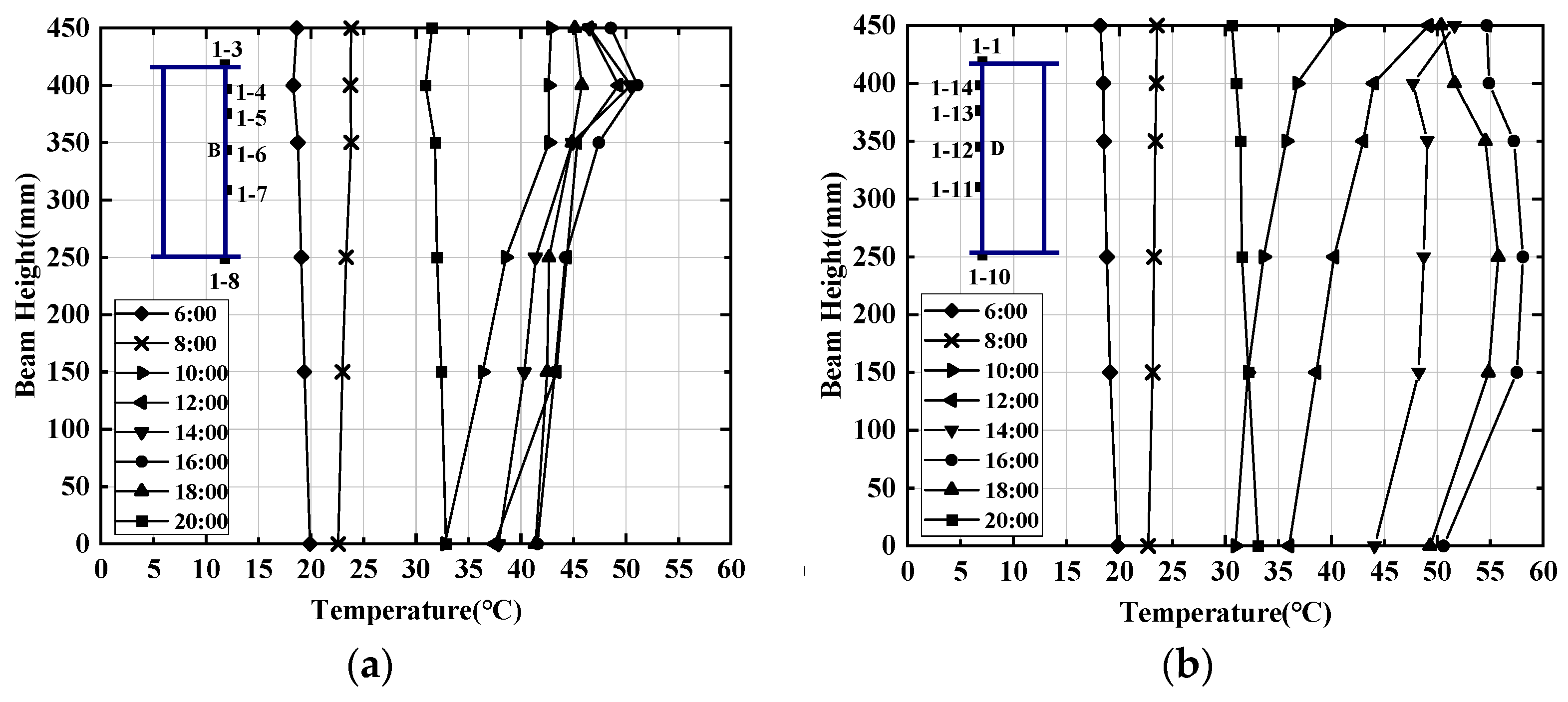
3.3. Changes in the Vertical Temperature Gradient
In order to further study and analyze the vertical temperature distribution of steel box girders, based on a large number of measured data, two sunny days, 30 July and 26 December, were selected as the representative days of summer and winter. According to the period from 6:00 to 20:00 on the same day, for plate B (measurement points 1-2, 1-4~1-7, 1~9 of the east web) and plate D (measurement points 1-2, 1-11~1-14, 1-9 of the west web) monitoring data, the temperature field of the steel box girder was analyzed, and the time step was 2 h.
In July, the sunrise in the Pingyao area appears at 6:00 a.m., midday occurs around 13:00, and sunset is around 19:30. As shown in
Figure 6, during the period from 6:00 to 8:00, the vertical temperature distribution of the steel box girder was relatively uniform, and the temperature difference was negligible. From 10:00 to 12:00, plate B on the east side was first irradiated by sunlight. As the sun rose, the top plate’s direct sunlight area increased, and the area of the bottom plate that was receiving the reflected radiation from the ground increased, so the temperature of both increased significantly. Since direct radiation efficiency is higher than reflection efficiency, the temperature of the top plate rises faster than that of the bottom plate. The maximum temperature difference occurs between 12:00 and 13:00. During the period from 14:00 to 18:00, with the change in the sun’s azimuth, the area of plate D exposed to direct sunlight increases, and the solar radiation is strong during this period, so the temperature in the middle of the web is higher. After 19:00, the vertical temperature tends to be uniform. At 20:00, the vertical temperature distribution of the steel box girder is relatively uniform, and the temperature difference is not significant.
Sunrise in winter is later than in summer, and sunset is earlier than in summer. From 10:00 to 18:00, the vertical temperature distribution of the steel box girder changed significantly, but the overall vertical temperature distribution and the rule of change with time were consistent with summer. However, due to the influence of the ambient temperature, the temperature rise in the top plate and the web plate of the steel box girder, and the temperature difference between the top plate and the bottom plate, were smaller than those in summer, as shown in
Figure 7.
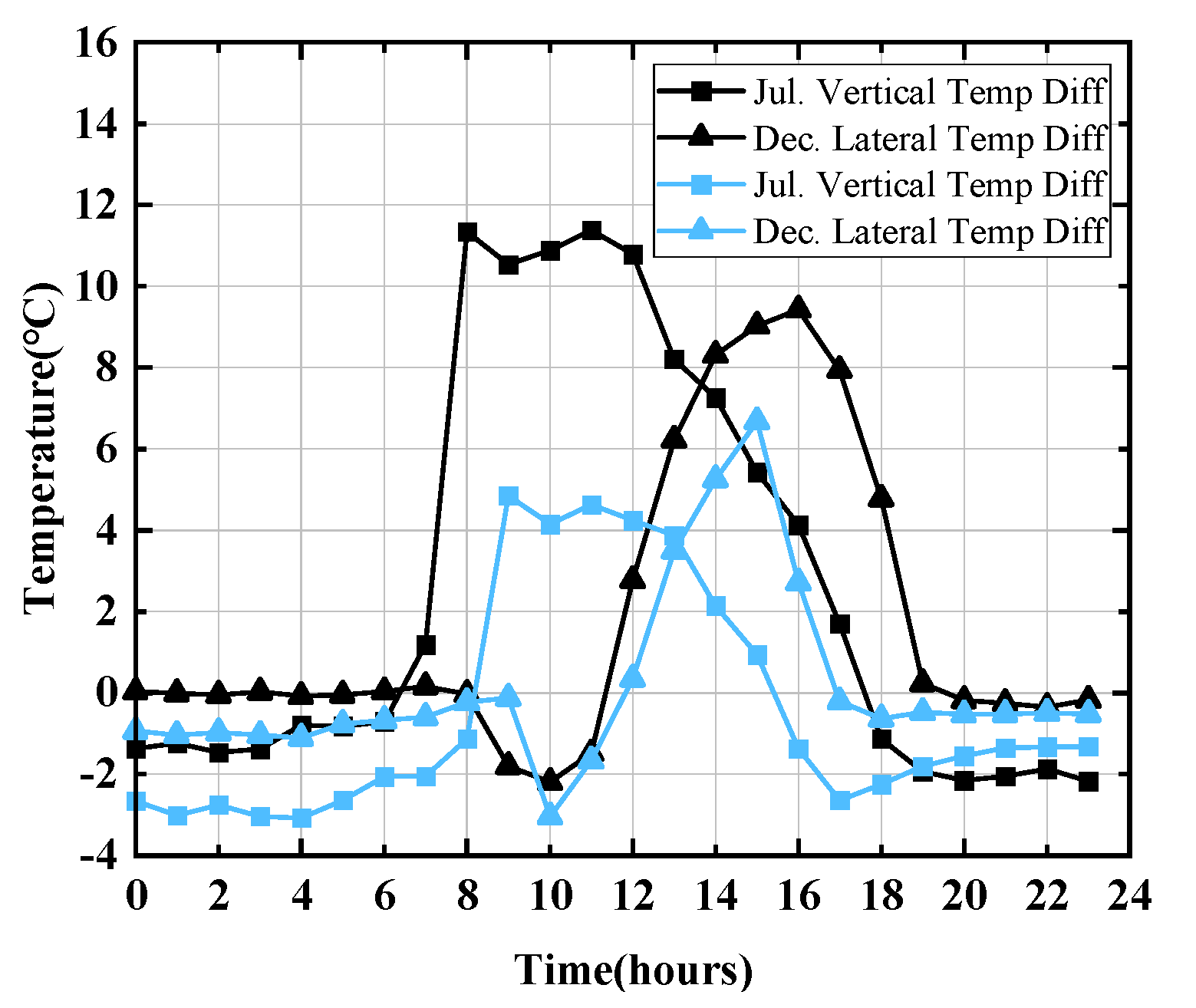
3.4. Law of Change in Temperature Difference
This section uses the temperature monitoring data of the top and bottom plates of the steel box girder on 30 July 2021 and 26 December 2021, to analyze the daily variation in the vertical and horizontal temperature differences. Considering that solar radiation is the most sensitive factor for the vertical temperature gradient distribution of the steel box girder, the difference between 1-2 and 1-9 is selected as the vertical temperature difference, and the difference between 1-10 and 1-8 is selected as the lateral temperature difference.
As shown in
Figure 8, the maximum vertical temperature difference in the steel box girder appears between 8:00 a.m. and 9:00 a.m., and the maximum lateral temperature difference appears around 15:00. The maximum vertical temperature difference in the summer is 11.38 °C, while the maximum horizontal temperature difference is 9.42 °C, which is about 82% of the vertical temperature difference, and the maximum horizontal temperature difference in winter is about 70% of the vertical temperature difference. In general, the lateral temperature difference in the steel box girder is much smaller than the vertical temperature difference but, due to the particularity of the cross-sectional size of the monorail track beam, the change in the angle of solar radiation leads to a sizeable lateral temperature difference.
The diurnal variation of the steel box girder in summer is similar to that in winter. The temperature difference changes less before 6:00 than after. During the period from 6:00 to 18:00, the temperature difference becomes more significant due to the change in the sun’s orientation and the change in the radiation intensity, respectively. After 18:00, the temperature difference tends to be stable. During the period from 9:00 to 11:00, when the sun passes directly above the components, the reflected radiation of the bottom plate is weakened, due to the influence of the steel box girder itself. However, with the change in the angle of the solar radiation, the reflected radiation received by the bottom plate gradually increases. Therefore, the temperature difference changes from small to large.
4. Temperature Gradient Curve
4.1. Temperature Gradient in Various Specifications
Table 1 shows the TB 10092-2017, GB/T 51234-2017, BS 5400, BS EN1991-1-5-2003, AASHTO, JTG D60-2015, the New Zealand Bridge Design Code, and the Australian Code [
18,
19,
20,
21,
22,
23,
24] for the provisions of the temperature gradient.
AASHTO, the Australian Code, the New Zealand Code, BS EN1991-1-5-2003, and JTG D60-2015 all pertain to steel beams with pavement and are unsuitable for pavement without bridge decks. TB 10092-2017 applies only to concrete structures. All of the six codes above lack provisions for the form of unpaved steel beams. The factors considered in BS 5400 are also comprehensive and give the temperature gradient load values under various working conditions of steel box girders without pavement, and pavement with different thicknesses. However, considering the differences in factors such as sunshine intensity, meteorological conditions, and the geographical environment, BS 5400 is not suitable for structural design in China. GB/T 51234-2017 gives the temperature gradient for pure steel beams, but the specification is based on BS EN1991-1-5-2003, considering a reduction factor of 0.8. The value of BS EN1991-1-5-2003 considers the pavement layer of 40 mm, but the bridge deck of the rail transit bridge is the lower layer; the width and thickness of the upper track structure are relatively large, and its shading effect has an impact on the vertical temperature gradient of the beam section. The reduction effect is noticeable and the value is too small. It can be seen that these two types of specifications also do not apply to the gradient temperature load design of unpaved steel beams in the monorail travel system.
4.2. Temperature Gradient in Various Specifications
This section discusses the positive and negative temperature difference curve forms suitable for the temperature gradient of unpaved steel beams, based on the measured data.
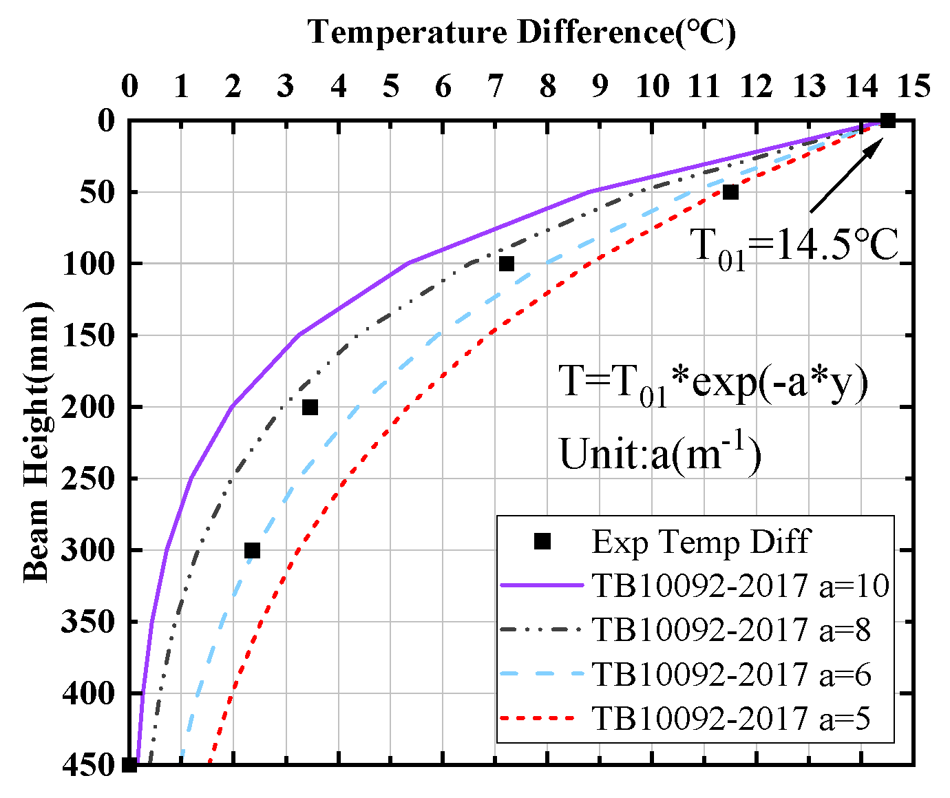
4.2.1. Positive Temperature Difference Curve
The positive temperature difference curves of the temperature gradients in various specifications are mostly multi-segment broken lines, and the exponential curves in TB 10092-2017 also have prominent nonlinear characteristics in the vertical direction. Therefore, we chose the exponential curve form and the multi-segment broken line form in GB/T 51234-2017 to fit and analyze the measured data to determine the temperature gradient curve form suitable for this study. The most negative vertical temperature gradients in a year usually occur in the summer when the solar radiation is the strongest. The maximum measured temperature gradient data on 4 July, a typically sunny day, were selected for fitting and analysis with the above two curve forms. The temperature gradient curve should take the zero point at the bottom plate and the maximum temperature difference at the top plate. Below, we discuss the effect of fitting with different values of the parameter a.
As shown in
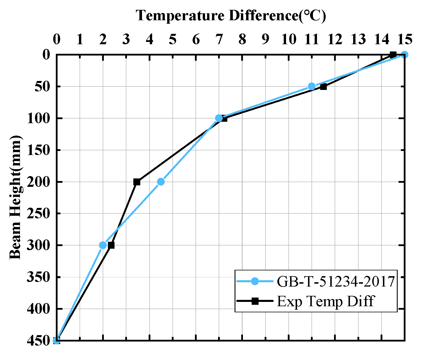
Figure 9, when a = 10, the curve basically satisfies the requirement that the temperature difference data at the bottom plate are the zero point of the temperature gradient curve, but the data of the four positions of the fitted curve web are very different from the measured data. The smaller the value of a, the more significant the offset of the backplane data to the zero point. When a = 6, the web position data fit well, but the zero offset is large. Therefore, using the exponential curve to fit the temperature gradient of the unpaved box girder is not suitable. The fitting effect of the multi-segment polyline temperature gradient model in GB/T 51234-2017, and the measured data of the box girder, are shown in
Figure 10. The maximum difference between the measured value and the multi-segment polyline model is 1.05 °C. Therefore, the multi-segment polyline curve model has a better fitting effect on the measured data of the unpaved steel box girder.
4.2.2. Negative Temperature Difference Curve
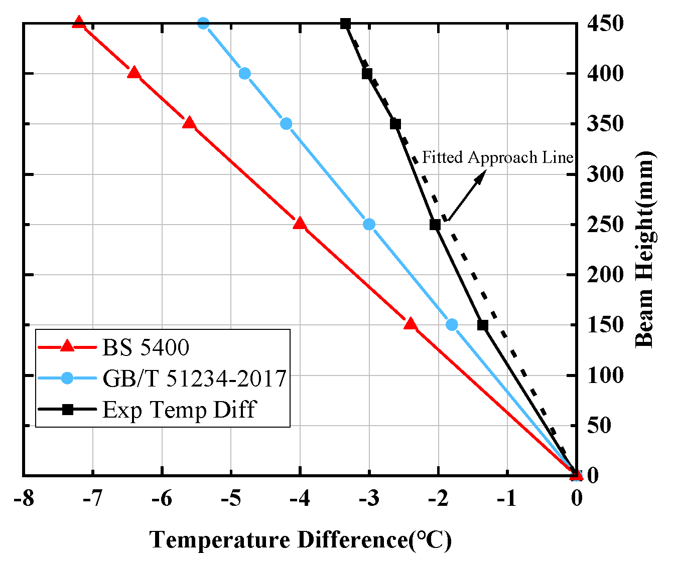
The negative temperature difference curves in various specifications are represented mainly by simple linear straight lines. GB/T 51234-2017 and BS 5400 give the negative temperature gradient model of the unpaved steel beam’s temperature gradient. We compared the temperature gradient model with the measured data. As shown in
Figure 11, the negative temperature difference distribution in the unpaved steel girder gradient temperature load is more consistent in form with BS 5400 and GB/T 51234-2017, so a linear straight line is used as the negative form of the temperature difference curve for the unpaved steel box girder.
4.3. Extreme Value Analysis of the Representative Value of the Temperature Difference
Extreme value theory predicts the probability of more extreme events in the future through the statistical analysis of extreme historical events. In this paper, extreme value theory predicts the most extreme temperature effects that may occur during the design life of steel box girder structures. In practical engineering applications, considering that the service life of the design of straddle-type monorail tourism systems is generally long, it is more appropriate to use generalized extreme value (GEV) distribution to perform extreme value analysis on the representative value of temperature differences.
4.3.1. Generalized Extreme Value Distribution
The distribution function of the generalized extreme value distribution:
where
μ is the position parameter,
σ is the scale parameter, and
ξ is the shape parameter.
Distribution type: when ξ→0, Gumbel distribution; when ξ > 0, Fréchet distribution; when ξ < 0, Weibull distribution.
4.3.2. Parameter Estimation and Model Checking
In order to obtain the representative value of the temperature difference of T
1 and T
2, based on the finite element thermal analysis model, the collected historical meteorological statistical data (from the US National Climatic Data Center, NCDC [
25]) were used as input parameters, and the “historical data” of the sunshine temperature field of the steel box girder in the Pingyao area were obtained through simulation analysis. The daily absolute maximum values of T
1 and T
2 from 1964 to 2021 were obtained, constituting a total of 58 years of sample data, considering reliability theory. The authors performed parameter estimation and model testing of the GEV distribution on T
1 and T
2 of the sample data and obtained the parameters and covariance matrices that the absolute values of T
1 and T
2 obey, respectively. The distribution types are shown in
Table 2.
We substituted the parameters in
Table 2 into Formula (1) to obtain the corresponding cumulative distribution function.
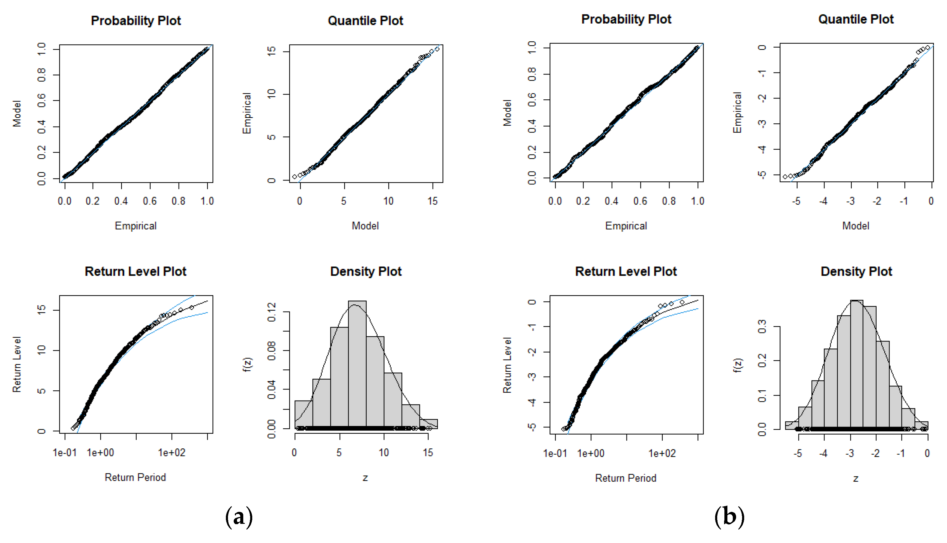
Figure 12 shows the test graphs obtained from the estimation of T
1 and T
2 parameters. The Weibull distribution can effectively describe the distribution patterns of T
1 and T
2.
4.3.3. Temperature Difference Representative Value
Under extreme environmental effects, the representative load-value of bridges and other structures is often described by the return period. The return period represents the average number of time intervals over which an extreme event recurs. The probability of this extreme event occurring is equal to the inverse of the return period. Assuming the random variable
X, the load representative value
with a return period of m years should satisfy.
where
n is the number of data points that
X can take in one year.
For the GEV distribution model, by substituting the distribution function (1) into Equations (2) and (3), the load representative value
with a return period of m years is shown to be:
In this paper, the representative temperature values with a return period of 50 years and 100 years were calculated, respectively, corresponding to the two cases of the design’s service life, 50 years and 100 years. By taking
m = 50,
n = 365, and
m = 100,
n = 365, respectively, and substituting them into Formula (3), the corresponding frequency
p = 0.00548% for the 50-year return period and
p = 0.00274% for the 100-year return period were obtained. We then substituted the extreme value distribution parameters in
Table 2 and the
p-values corresponding to different return periods into Equations (4) and (5). The representative values of T
1,ref and T
2,ref for the unpaved steel box girders T
1 and T
2 of the 450 mm beam height of the monorail tourism system in the Pingyao area are shown in
Table 3.
4.4. Temperature Gradient Curve Model
In order to establish a complete temperature gradient model, it is necessary to determine the value of the temperature base in the curve. The results of the calculation of the maximum temperature difference representative values T1 and T2 can be obtained from the information above. In order to determine the value of the temperature base T04 in the temperature difference curve, based on the finite element model, the changes in the temperature difference more significant than 600 mm from the top of the beam are calculated.
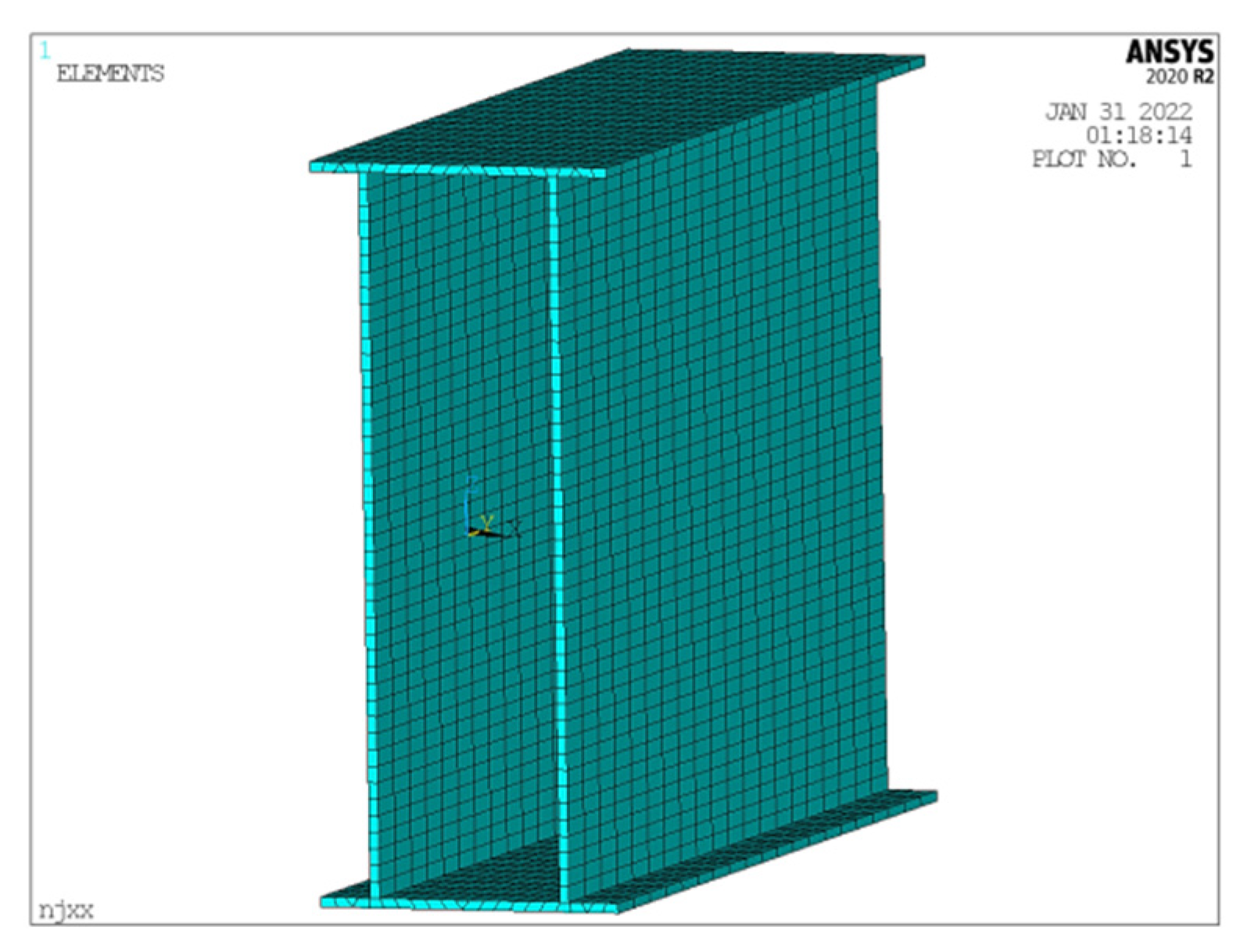
4.4.1. Finite Element Model
According to the actual size of the specimen, the finite element calculation model is established by the APDL [
26] parameterization in ANSYS, and the three-dimensional solid element SOLID 70 is selected. SOLID70 is an eight-node tetrahedral element with only one degree of freedom of temperature at each node. The entire steel box girder model has a total of 5418 nodes and 2640 elements. The cell division is shown in
Figure 13. The ASHRAE [
27] clear-sky model is used to determine the calculation parameters of the solar radiation intensity and boundary conditions of the steel box girder temperature field.
Table 4 shows the physical parameters of the steel, and
Table 5 shows the numerical simulation parameters of the temperature field. Among them, the radiation emissivity of steel is taken as 0.6; the surface solar radiation absorption coefficient is taken as 0.75; the reflectivity of the ground or horizontal plane is taken as 0.35; and the solar radiation intensity A, when the air mass is 0, is taken as 1367 W/m
2.
The temperature field variation of the unpaved steel box girder was studied using the transient analysis method. The TUNIF command was used in APDL to set the initial temperature value. It can be seen from the actual test that the overall temperature of the steel box girder tended to be uniform around 6:00 in the morning, and the overall temperature at that time was taken as the initial temperature field. Among the three forms of heat exchange between the steel beam and the outside world, the convective load was applied by assigning the atmospheric temperature and the convective heat transfer coefficient to each boundary surface. The long-wave thermal radiation is considered to be equivalent to a convective load in order to simplify the calculation. Solar radiation is applied in the form of a heat generation rate equivalent to the body load. In this paper, 6:00 was selected as the initial time in the transient temperature field analysis, the sunshine temperature field analysis time range was 6:00–20:00, the load-step time was 3600 s, and the number of load-substeps was 60.
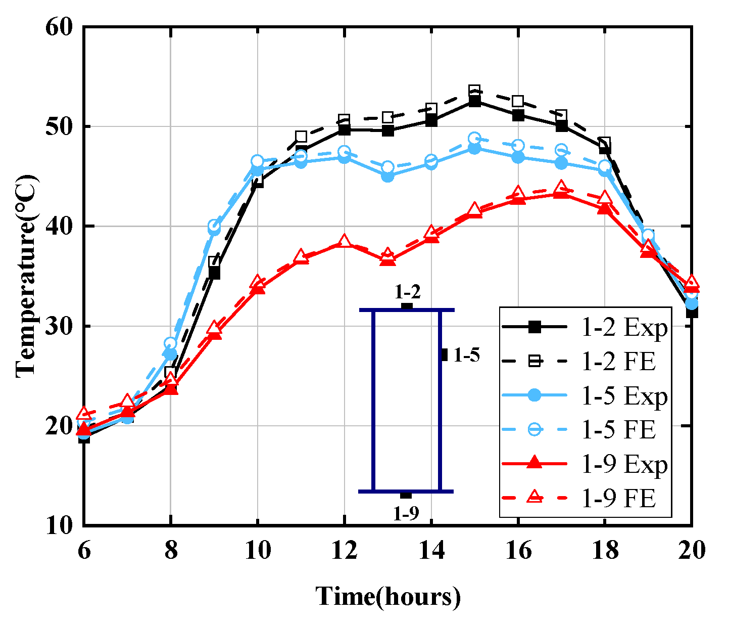
4.4.2. Model Validation
In order to verify the correctness of the ANSYS calculation model, taking the data of 30 July 2021 as an example, the author compared the calculated temperature of the vertical part of the steel box girder with the measured temperature. The results of the comparison are shown in
Figure 14.
Figure 14 shows that the maximum deviation between the calculated value and the measured value of the corresponding measuring point of the steel box girder is within 5%. The results show that the model can accurately simulate the temperature field change in the steel box girder, and the calculated value of the structural transient temperature field is shown to be in good agreement with the measured value.
4.4.3. Complete Temperature Gradient Model
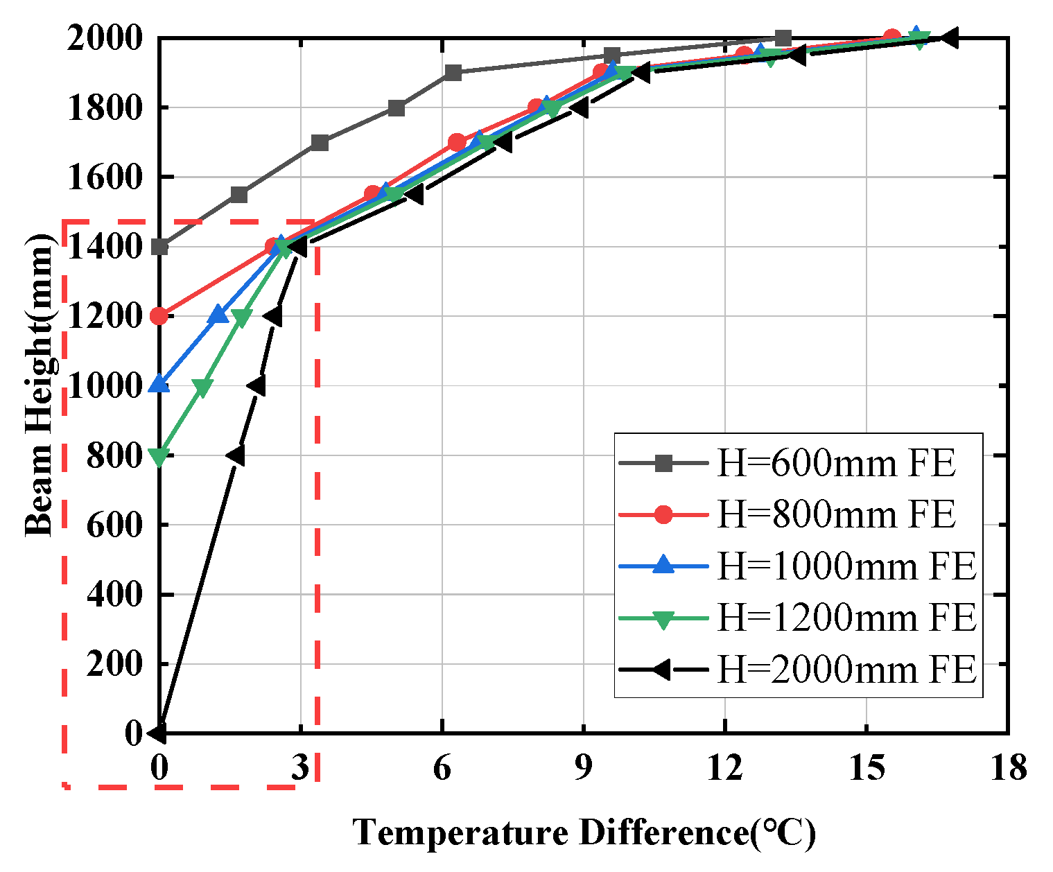
Based on the finite element model, the temperature difference changes beyond the range of 600 mm from the top of the beam are calculated, and the temperature gradient distributions of five different beam heights of 600 mm, 800 mm, 1000 mm, 1200 mm, and 2000 mm are compared.
Figure 15 shows that the temperature difference outside the range of 600 mm from the top of the beam is within 3 °C, so T
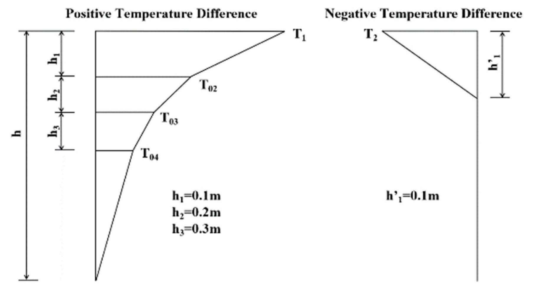
04 = 3 °C. The temperature gradient is divided into four parts along the direction of the beam height:
= 0.1 m,
= 0.2 m,
= 0.3 m, and
-0.6 m. Among them, the temperature difference change value within the range of
from the top accounts for about one-half of the difference between T
1 and T
04, and the temperature difference change value within the range of
accounts for about three-fifths of the difference between T
02 and T
04.
Figure 16 shows the complete temperature gradient model, and
Table 6 shows the temperature base values for different return periods.
5. Conclusions
In this paper, an experimental study was carried out on the sunshine temperature field of an unpaved steel box girder in a monorail travel system, and the behavior of the temperature change in the unpaved steel box girder was analyzed, based on long-term measured data. The representative value of the temperature difference between the 50-year return period and the 100-year return period of the beam, with a height of 450 mm, was predicted using the GEV distribution, and the temperature gradient model of the unpaved steel box beam was determined. The conclusions based on this study are as follows:
During the whole test cycle, the steel box girder’s maximum vertical positive temperature difference was 15.21 °C, and the negative temperature difference was −5.07 °C. An important factor affecting the vertical temperature difference distribution is the effect of the ambient temperature, considering the solar radiation.
Compared with the ambient temperature, the temperature of each measuring point has an apparent time-lag phenomenon. The representative temperature of the specimen has an obvious correlation with the daily maximum ambient temperature, and the changing trend between the two is the same.
The comparative analysis of the temperature gradient curves of various specifications shows that the positive and negative temperature difference curves of the unpaved steel box girder in this paper are multi-segment broken lines and linear straight lines, respectively.
Based on historical meteorological data, combined with the long-term “historical data” of the temperature field of unpaved steel beams, calculated by the finite element model, a generalized extreme value distribution model was used for the analysis of extreme values. The prediction of extreme values was carried out using the historical data of the temperature load, the parameter estimation value and distribution type of the extreme value model were determined, and the representative values of the temperature difference for the 50-year return period and the 100-year return period were obtained. Finally, the most negative temperature gradient in the design service life was determined, the temperature-gradient model of the unpaved steel box girder was established, and the value of the temperature base was given to provide a reference for related structural designs.


