Real-Time Strawberry Plant Classification and Efficiency Increase with Hybrid System Deep Learning: Microcontroller and Mobile Application

Abstract

The strawberry plant has three life stages: seedling, blooming, and crop. It needs different acclimatization conditions in these life stages. A dataset consisting of 10,000 photographs of the strawberry plant was prepared. Using this dataset, classification in convolutional neural networks was performed in Matrix Laboratory (MATLAB). Nine different algorithms were used in this process. They were realized in ResNet101 architecture, and the highest accuracy rate was 99.8%. A low-resolution camera was used while growing strawberry plants in the application greenhouse. Every day at 10:00, a picture of the strawberry plant was taken. The captured image was processed in ResNet101 architecture. The result of the detection process appeared on the computer screen and was sent to the microcontroller via a USB connection. The microcontroller adjusted air-conditioning in the greenhouse according to the state of the strawberry plant. For this, it decided based on the data received from the temperature, humidity, wind direction, and wind speed sensors outside the greenhouse and the temperature, humidity, and soil moisture sensors inside the greenhouse. In addition, all data from the sensors and the life stage of the plant were displayed with a mobile application. The mobile application also provided the possibility for manual control. In the study, the greenhouse was divided into two. Strawberries were grown with the hybrid system on one side of the greenhouse and a normal system on the other side of the greenhouse. This study achieved 9.75% more crop, had a 4.75% earlier crop yield, and required 8.59% less irrigation in strawberry plants grown using the hybrid system.

1. Introduction

Strawberries are a fruit species grown in a wide variety of ecological conditions across the world, and strawberry production is increasing every year. Strawberry cultivation is generally done with traditional agriculture in soil. Production with traditional agriculture causes many diseases and production efficiency is not very high. The yield is very high when production utilizes soilless agriculture in greenhouses. Strawberry plants grow very quickly when grown in greenhouses. This means that the needs of strawberry plants change very quickly. The faster the response to the situation, the higher the yield of the strawberry will be. Using deep learning, fast and very highly accurate detection can be achieved. There are many studies with deep learning in the literature.

Kawasaki et al. studied cucumber leaves. They tried to detect leaf diseases in cucumbers. A total of 7520 samples were tested in their study. Half of the photographs used in their sampling were taken in poor conditions. As a result of this study, they obtained an accuracy rate of 82.3% with convolutional neural networks [1]. Sladojevic et al. worked on disease detection by using leaf images. They identified 13 different classifications in their study. In this study, they used more than 30,000 samples for convolutional neural networks. They reached an accuracy rate of 91.11% in the experimental study [2]. Mohanty et al. used a publicly available dataset. In that study, the dataset consisted of 54,306 images and detected 26 diseases. Convolutional neural networks were also used in that study. As a result of their study, they reached an accuracy rate of 99.35% in an extended test set of [3]. Nachtigall et al. worked on the detection of 6 diseases in apple trees. They used a dataset of 2539 images in their study. As a result of their study, they achieved an accuracy rate of 97.3% at the best performance [4]. DeChant et al. worked on the detection of northern leaf blight disease in maize plants. In that study, they used a dataset consisting of 1796 images. They reached an accuracy rate of 96.7% with the dataset that they used [5]. Lu et al. studied rice diseases. Their work was on the detection of 10 common rice diseases. The dataset used in their study consisted of 500 images. They reached an accuracy rate of 95.48% with a CNN-based model [6].

Brahimi et al. worked on the detection of general diseases in plants. They used AlexNet and GoogleNet architectures in convolutional neural networks in their studies. They used a dataset consisting of 14,828 images in their study. In their studies, they reached an accuracy rate of 97.35% with AlexNet and an accuracy rate of 97.71% with GoogleNet [7]. Rangarajan and his friends worked on the detection of diseases in tomatoes. In their study, the detection of six diseases was performed and images of one healthy tomato were used. There were 13,262 images in the dataset that they used. VGG16 and AlexNet architectures were used for the detection of diseases. In that study, 97.29% accuracy was obtained with VGG16 and 97.49% accuracy was achieved with AlexNet [8]. Khandelwal and Raman studied general diseases in plants. In their study, ILSVRC 2012 architecture was used in convolutional neural networks on a dataset consisting of 86,198 images. The results of their study reported that an accuracy rate of 99.37% was reached [9]. Waheed et al. worked on corn plants. They tried to detect diseases that occur in maize plants with convolutional neural networks. DenseNet architecture was used in convolutional neural networks in that study. The results of their study reported that they reached an accuracy rate of 98.06% [10]. Epinso et al. performed work on solar panels. In their study, they tried to identify two classifications of solar panels: defective and intact. Convolutional neural networks were used in their classification. They used 345 images in their study. The results of their study report that they reached an accuracy rate of 70% [11]. Tang et al. worked on the detection of diseases in grapes. They used convolutional neural networks in their work. A total of 4062 grape leaf pictures were used as the dataset in their studies. They created four classifications: one healthy and three disease. They used a ShuffleNet architecture. An accuracy rate of 99.14% was found in the best-trained learning model [12]. Wang et al., while working on the detection diseases in rice, classified rice grains into four classifications: healthy rice and three groups of diseased rice. Their sample consisted of 503 grains of healthy rice, 523 with brown spots, 779 with leaf blast, and 563 with rice hispa damage. They used DenseNet121, VGG16, ResNet50, and MobileNet architectures in convolutional neural networks. The results of that study reported that MobileNet had an accuracy rate of 90.2% [13].

When the literature is examined, the studies are mostly on classification. Photographs of the plant were taken for classification. A dataset was created with these photographs. With this dataset, classification was performed in convolutional neural networks in MATLAB. In order to increase the accuracy rate, the photos of the plants were taken in a laboratory environment, not in real living areas. The classification process was carried out only in one phase of the plant. The most important feature of this study is that the classification process is not only carried out at one stage of the strawberry plant, but over the whole lifetime. The classification process is carried out from the planting of the strawberry plant as a seedling to the end of the crop yield. In this study, a high accuracy rate of 99.8% was achieved. The most important reason for this was a trial planting of the strawberry plants. The dataset consists of photographs of strawberry plants in this trial planting. Cocopeat was used in the trial planting and subsequent real planting. Thus, the similarity rate was increased in both cultivations. In this study, the real planting was performed in a greenhouse. For the classification process, a picture was taken every day at 10:00 in the morning with a low-resolution camera while the strawberry plant was growing in the greenhouse. This picture was tested with the ReNet101 architecture, which previously gave the highest accuracy rate of four different algorithms. The result of the process was transferred to the microcontroller via USB. The microcontroller adjusted the air conditioning in the greenhouse according to the state of the strawberry plant. To make this decision, it used the data received from the temperature, humidity, wind direction, and wind speed sensors outside the greenhouse and the temperature, humidity, and soil moisture sensors inside the greenhouse. In addition, all data from the sensors and the life stage of the plant were displayed with a mobile application. This mobile application also provided the ability for manual control. In this study, the greenhouse was divided into two. The hybrid system was grown on one side of the greenhouse and normal strawberries were grown on the other side. Thus, the comparison was made.

2. Materials and Methods

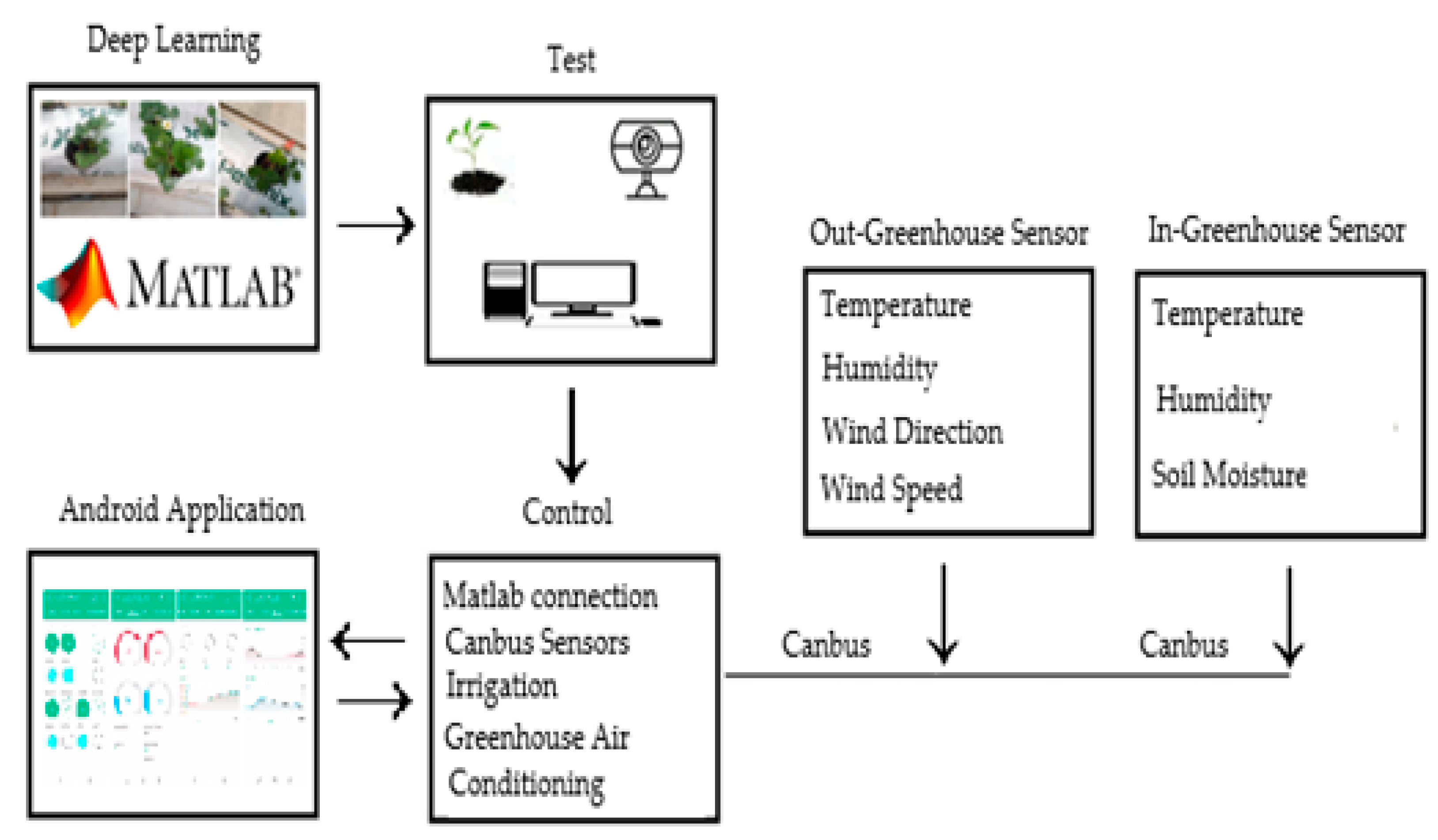
The study was carried out in three stages. Classification of three different growth stages of strawberry plant—seedling, flowering, and crop—was carried out. Secondly, this classification was applied in the real greenhouse. For this, the strawberries grown in the greenhouse were photographed every day at 10:00 in the morning. This photo was tested on the ResNet101 architecture. The result of this operation was sent to the Arduino microcontroller. The microcontroller adjusted air conditioning in the greenhouse according to the state of the strawberry plant. To make this decision, it used data from the temperature, humidity, wind direction, and wind speed sensors outside the greenhouse and the temperature, humidity, and soil moisture sensors inside the greenhouse. Finally, using a mobile application, all data from the sensors and the life stage of the plant were displayed. The mobile application also enabled manual control. Figure 1 shows the general structure of the system.

2.1. Dataset

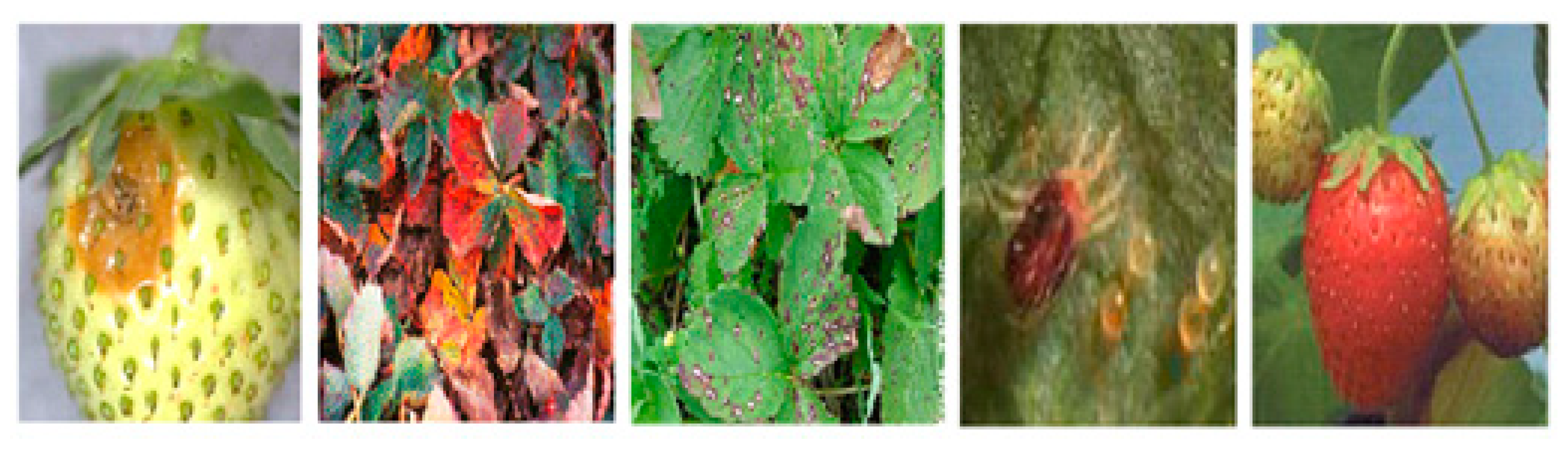
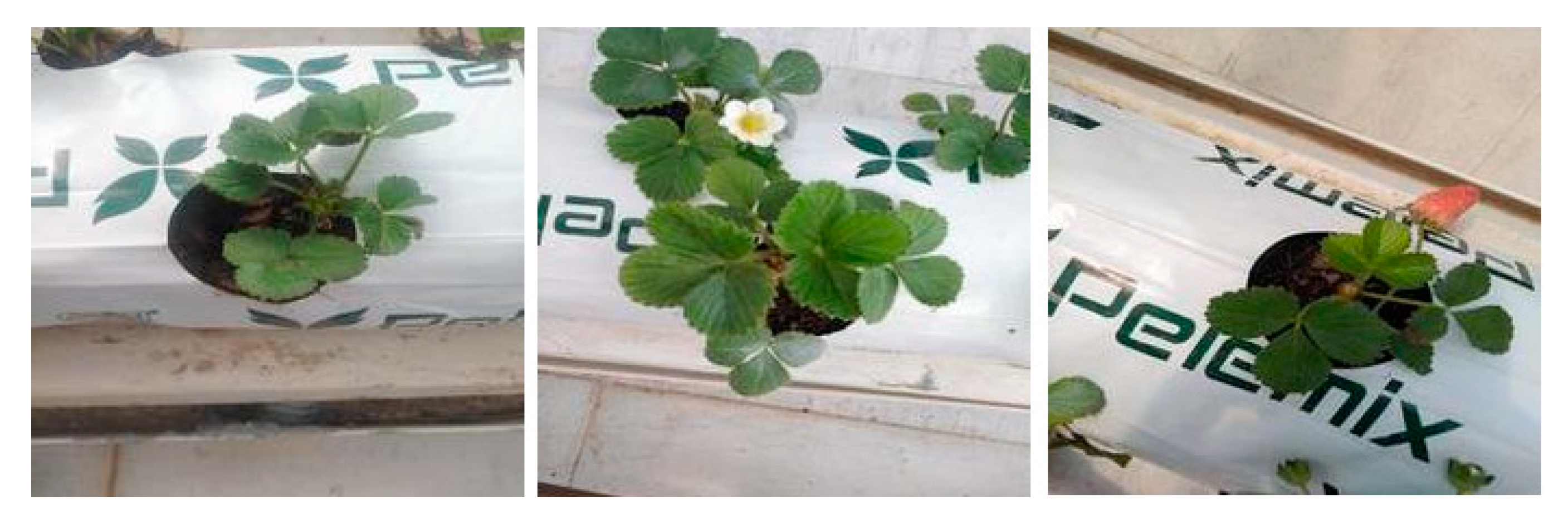
A dataset consisting of 10,000 photographs was used in the study. Trial cultivation was done for this dataset. The dataset consists of photographs obtained from the trial planting and photographs obtained from the outside greenhouses. The dataset includes five different diseased strawberry groups and three different growth stages of strawberry plants. Figure 2 shows three healthy photographs of the strawberry plant used in the dataset.

In this study, the process was controlled. For this, three healthy states of strawberry plant were determined. Trial sowing was performed to determine the status of the strawberry plants. Thus, the similarity of the photographs to be taken later in the greenhouse to the photographs that form the dataset was increased. No disease was detected in the strawberry plants during the trial planting. In this study, photos of diseased strawberries from the surrounding greenhouses and the internet were used. Figure 3 shows the diseased strawberry plant photos used in the dataset.

2.2. Deep Learning

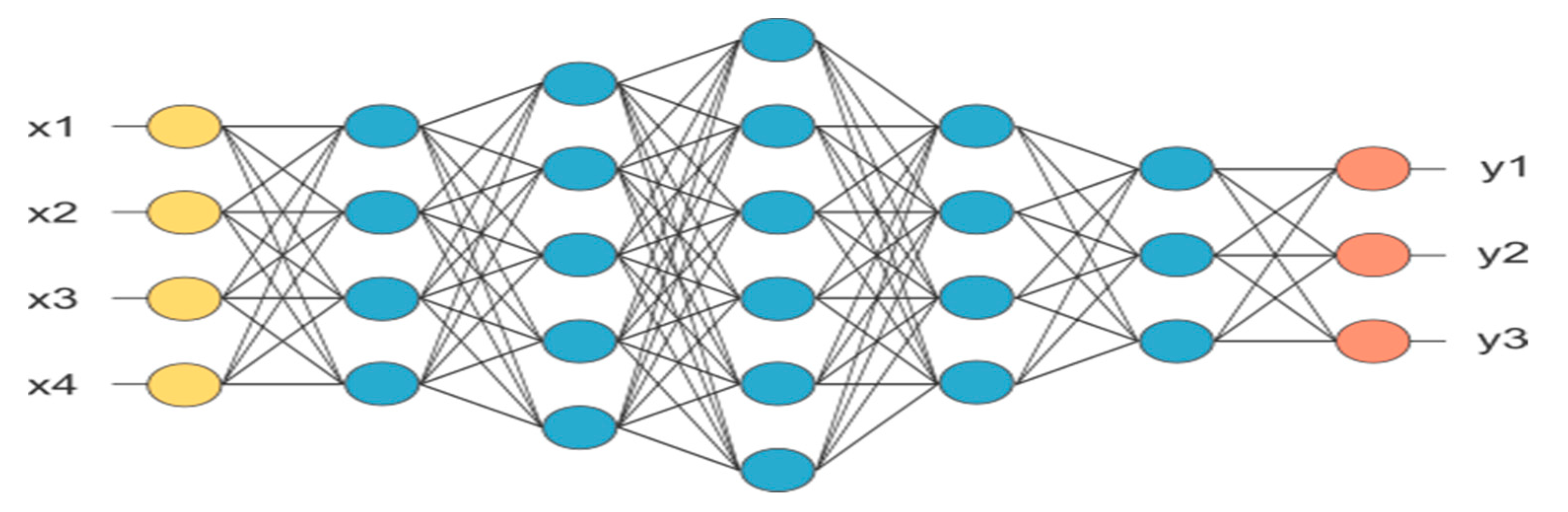
Deep learning is a field of study that covers artificial neural network algorithms with many hidden layers. The most well-known of the deep learning algorithms is the convolutional neural network algorithm. It is one of the most frequently used algorithms in image classification problems. The main structure of convolutional neural networks is based on computer vision and deep learning. CNNs obtain a different layered output by applying the specified filter to the image step by step. The CNN in this study was implemented in MATLAB to create the necessary layers of the CNN architecture. Figure 4 shows the architecture of a convolutional neural network.

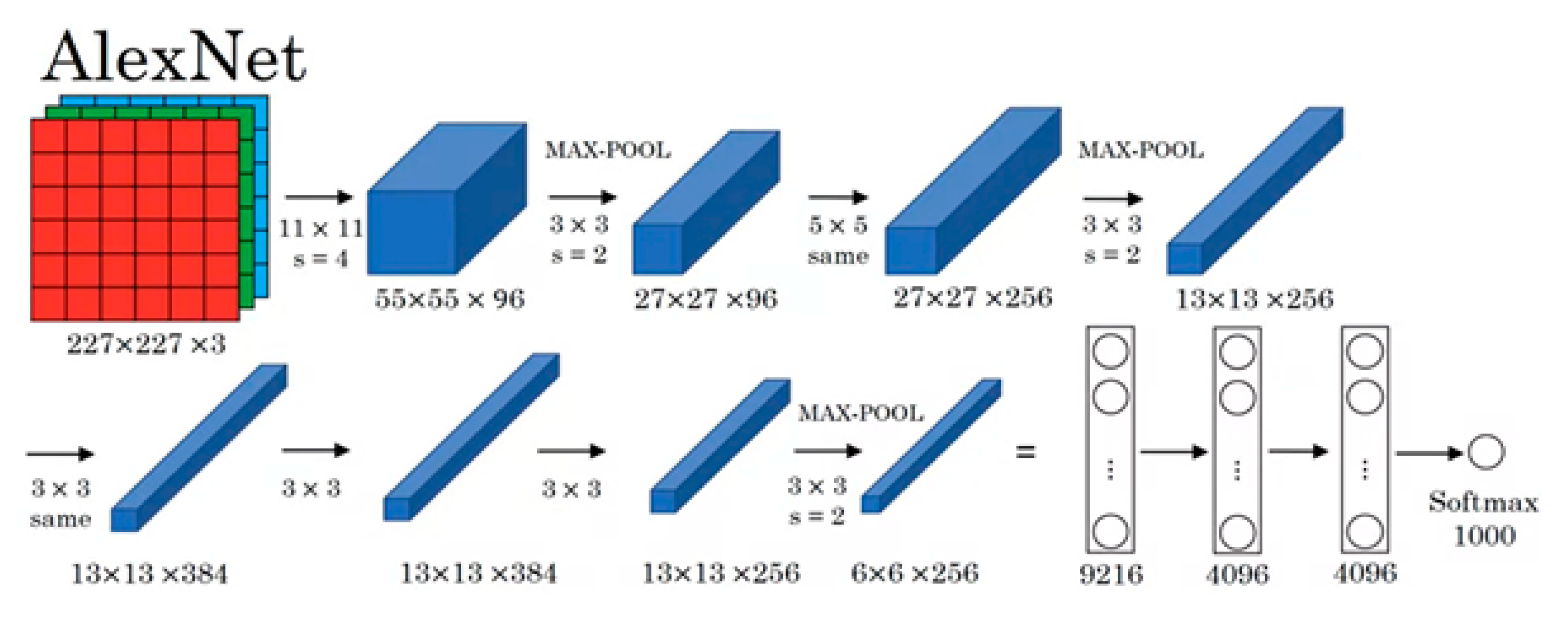
2.3. AlexNet

AlexNet was created by Alex Krizhevsky [14]. The AlexNet model won the ImageNet competition held in 2012 [15]. The input to AlexNet was a 256×256 RGB image. This means that all images and all test images in the training set must be 256×256. If the input image was grayscale, it was converted to an RGB image by multiplying the single channel to get a three-channel RGB image. It had 60 million parameters and 650,000 neurons. It took five to six days to train on two GTX 580 3GB GPUs. With this architecture, the computerized object identification error rate was reduced from 26.2% to 15.4%. The architecture was designed to classify 1000 objects. The filters were 11×11 in size and the number of step shifts was 4. The architecture given in Figure 5 consists of 5 convolution layers, a pooling layer, and 3 fully connected layers.

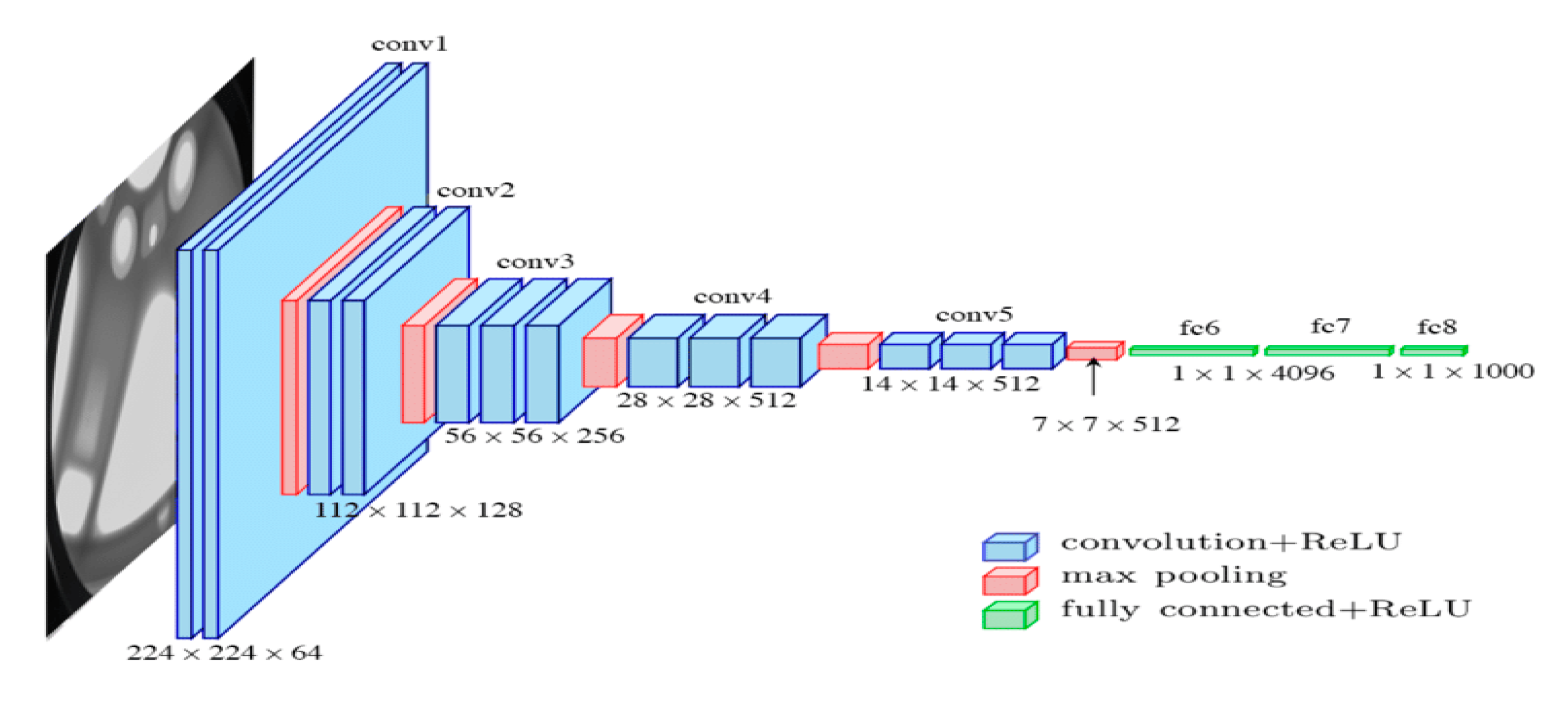
2.4. VGGNet

VGG Net was designed by Matthew Zeiler and Rob Fergus. They won the ImageNet competition held in 2013 [16]. With the designed VGG Net model, the error rate in object recognition was reduced to 11.2%. This architecture was an enhanced version of the AlexNet architecture and is shown in Figure 6.

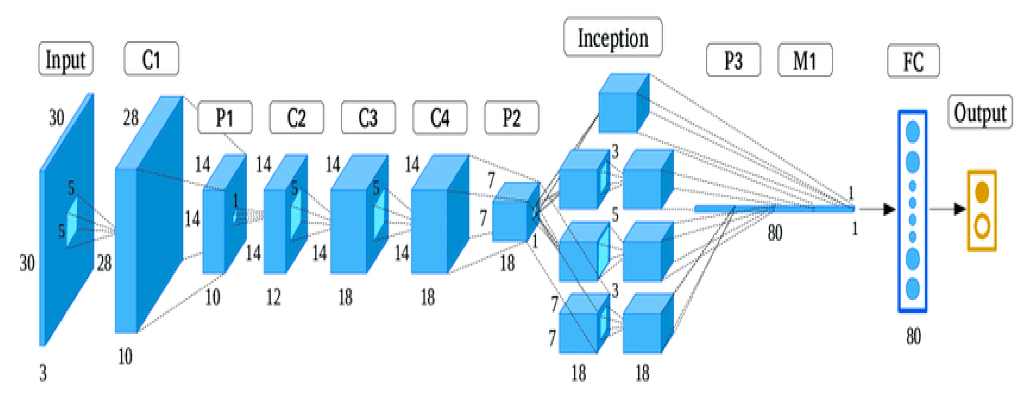
2.5. GoogleNet

GoogleNet was developed by Szegedy [17], who won the ImageNet competition held in 2015 [16]. GoogleNet has a complex architecture due to the incorporation of Inception modules. GoogleNet has 22 layers and a 5.7% error rate. The GoogleNet architecture was the first CNN architecture to move away from stacking convolution and pooling layers in a sequential structure [18]. Additionally, this new model represented an important advancement in memory and power usage, as stacking all the layers and adding many filters adds computational and memory costs and increases the probability of memorization. GoogleNet used modules connected in parallel to overcome this problem. The GoogleNet network architecture is shown in Figure 7.

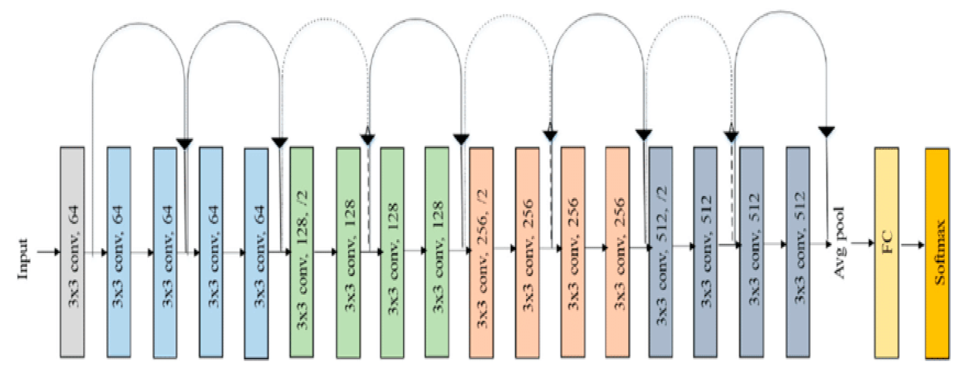
2.6. ResNet

ResNet was developed by He [19]. It was an architecture more deeply designed than all other architectures. It consisted of 152 layers and was also the winner of the ImageNet 2016 competition, with an error rate of 3.6%. Depending on their skills and expertise, humans generally had an error rate of 5–10%. ResNet’s first 34-layer network architecture is shown in Figure 8.

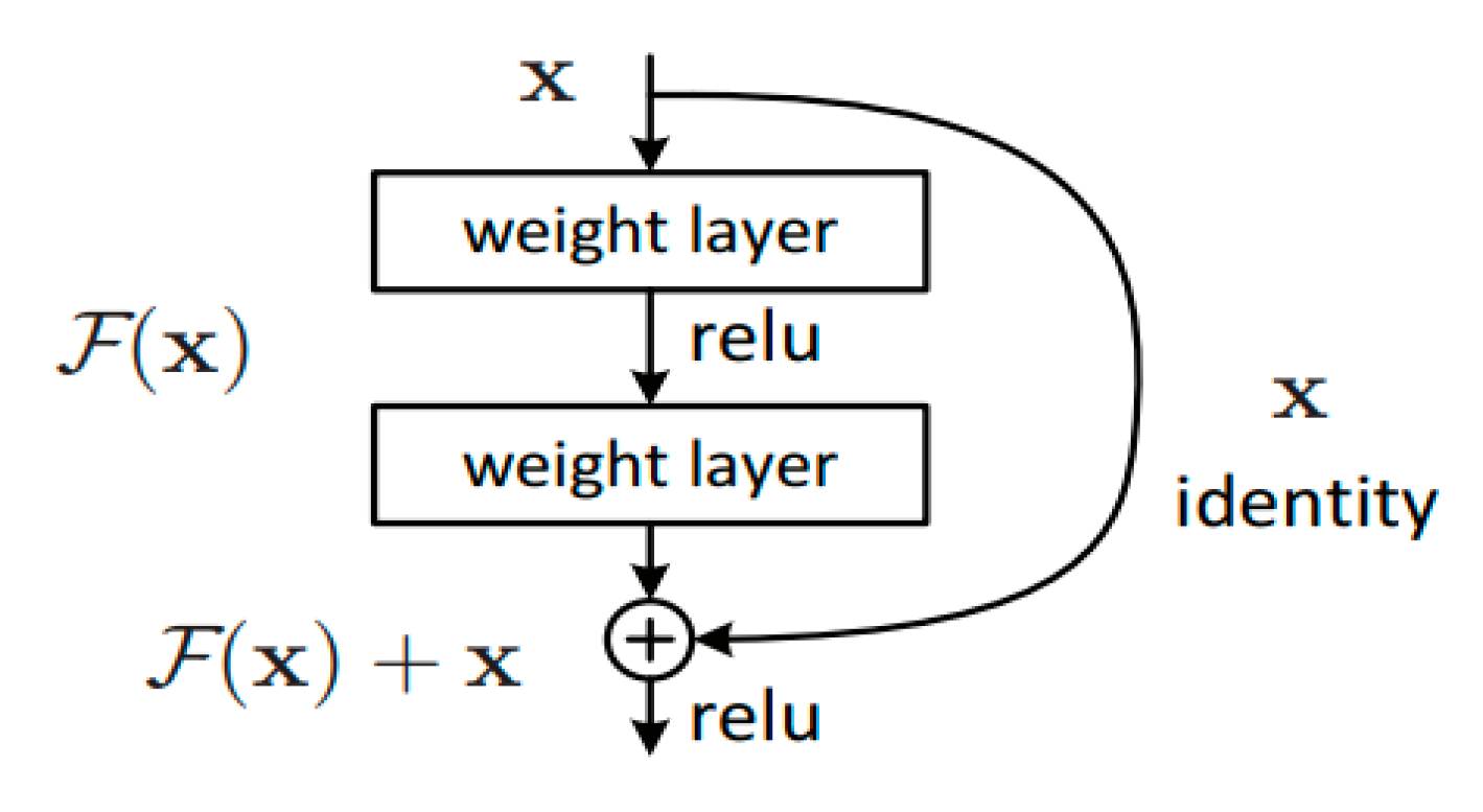
The ResNet architecture consisted of residual blocks. In the residual block, it gave an F(x) result after the convolution-ReLu-convolution series of input x. This result was then added to the original input x and expressed as H(x) = F(x) + x (Figure 9).

When the literature was examined, it was understood that the lowest error rate belongs to the ResNet101 architecture. With the increase in the convolution layer, the error rate decreased to a rate of 3.6%. Although the error rate of humans varied, it varied between 5–10% on average. This showed that ResNet101 architecture gives better results than humans.

2.7. Applied System

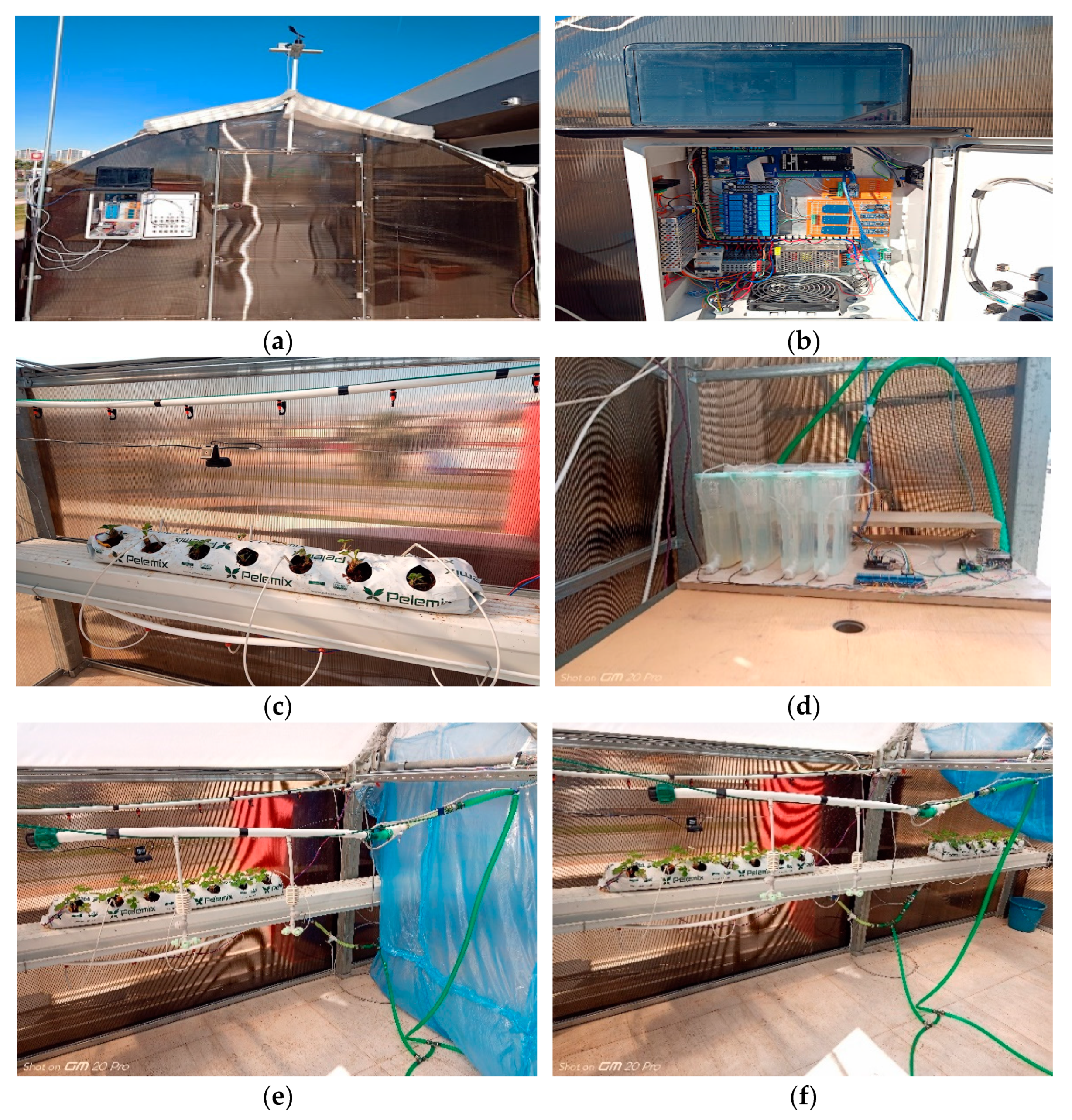
In this study, the diseases that may occur in the life process of the strawberry plant were determined. In doing this, deep learning was used. During this process, a webcam was fixated on the plant grown in the greenhouse. The webcam took pictures of the strawberry plant in the greenhouse at 10:00 every morning. This photograph was tested in the deep learning algorithm which gave the highest accuracy rate. This process took place in MATLAB. The result of the process was reported by communicating with the Arduino microcontroller. According to the treatment of the disease detected by the microcontroller, a chemical or chemical mixture was applied to the plant. According to the condition of the plant, the indoor climate is adjusted. In this way, both crop productivity and irrigation efficiency were increased with timely delivery of the required amount of irrigation and humidification. Figure 10 shows the realized system.

2.8. Mobile Application

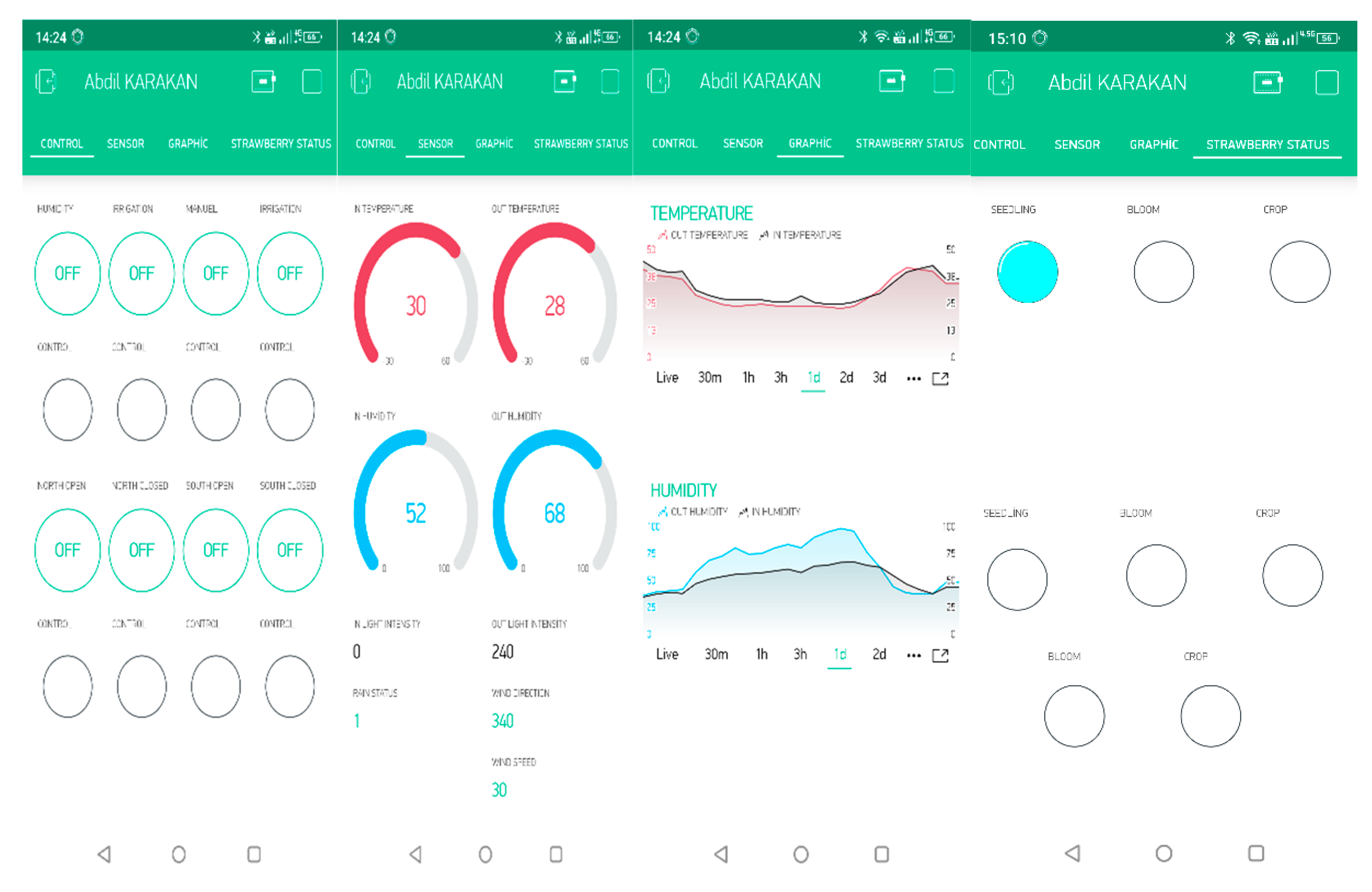
In this study, the system was monitored and controlled remotely. For this, an android application interface was designed. With this interface, all data produced by the system were displayed. In addition, remote control ability was also provided. Figure 11 shows the interface designed for the remote monitoring and control of the system.

The designed interface consists of four parts: control, sensor, graphic, and strawberry status. In the control section, the system can be controlled either manually or automatically. In this study, when manual control was selected, the north and south ventilation could be opened and closed, the irrigation and humidification of the strawberries grown with deep learning could be controlled, and the irrigation of the normal strawberry plants could be controlled. The control part of the interface provides feedback. When any button in the control part is pressed, the button is first activated and its color changes. The control light at the bottom changes according to the output of the microcontroller. The light is on when the output is active. Thanks to this feedback, it is possible to check whether the system is working or not. In the sensor section, data from sensors inside and outside the greenhouse are displayed. These are temperature, humidity, wind speed, wind direction, rain information, and luminous intensity. In the graphic section, the temperature and humidity values are displayed as instantaneous, 30 min, 1 h, 3 h, 1-day, and 2-day data. In the strawberry status pane, the life stage of the strawberry is shown. The fuzzy logic control values required for humidification are shown. The value from the soil moisture sensor is also displayed.

3. Results

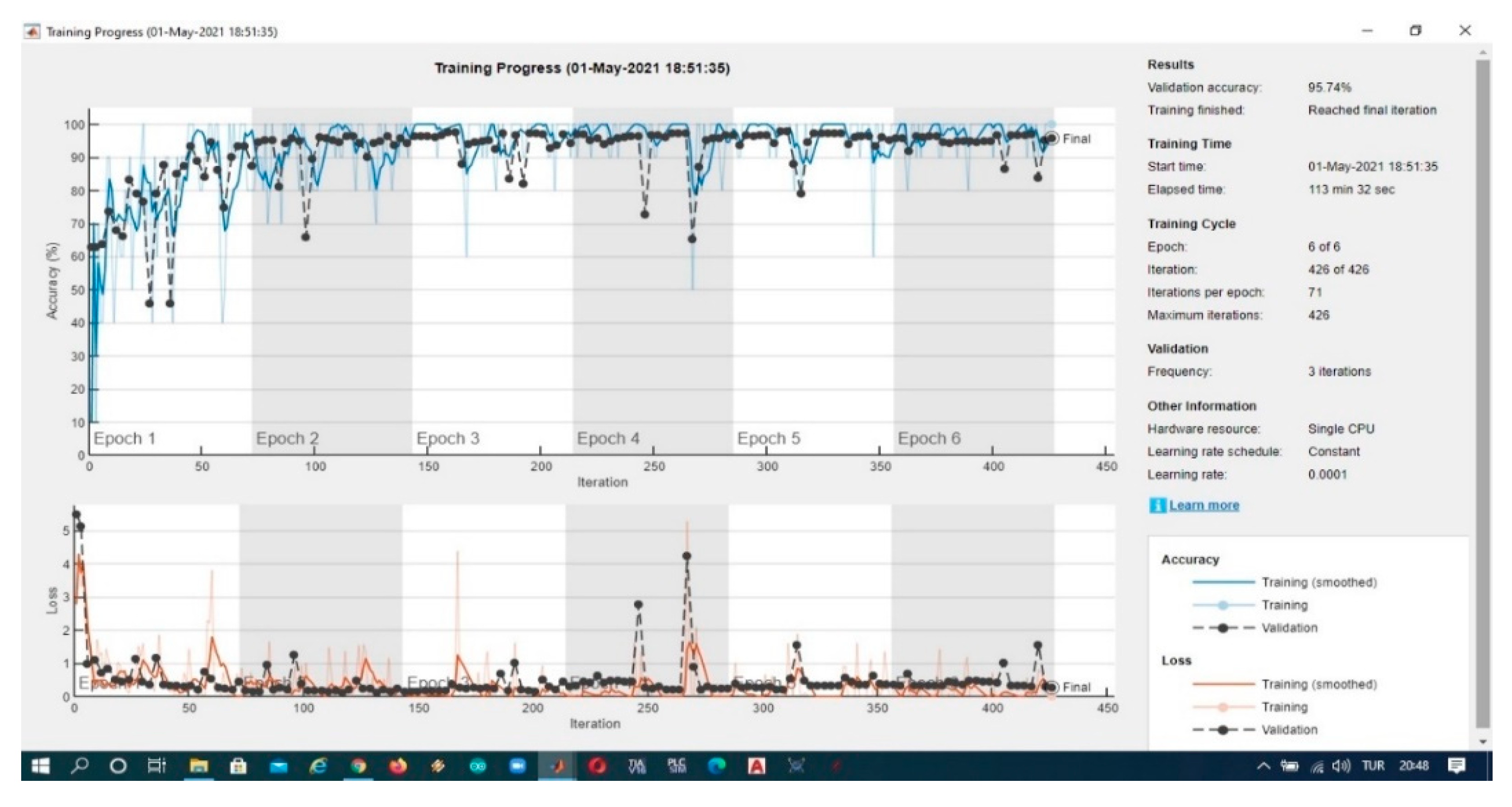
The study which is carried out here covers the complete production process. This process is 45 days from planting the strawberry plant to the crop time. In this study, 70% of the data were used for training and 30% of the data were used for testing. Figure 12 shows the training process of the AlexNet architecture used in the system.

AlexNet is one of the first architectures used in convolutional neural networks. In the AlexNet architecture, a photo with dimensions of 227 × 227 is used. The depth parameter is 6 million. The rate of error in the AlexNet architecture varies between 15.4% and 26.2%. The main reason for the high level of change in this rate is the dataset. The more similar the photos which made make up the dataset are, the lower the error rate is. In this study, a trial plant was created to minimize the rate of error. Using photographs from the planting seedling of the strawberry plant planting to the end of the crop stage in the trial planting, a dataset was created. Because of this, the accuracy rate was 95.74% and the rate of error was 4.26%. The detection error rate of a normal person varies between 5 and 10%; the AlexNet architecture reached a lower error rate than a normal person. 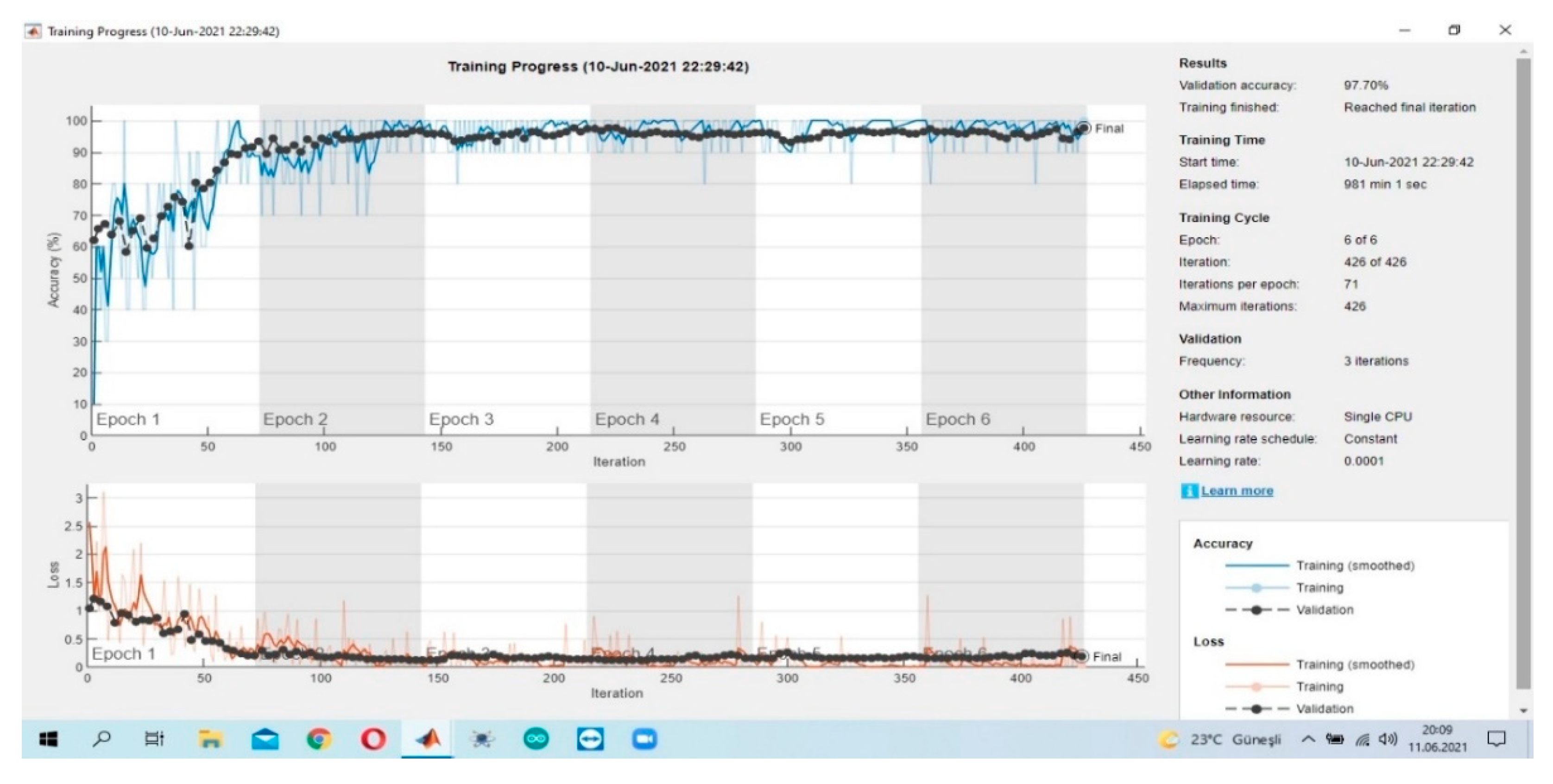Figure 13 shows the training process of the VGGNet architecture used in the system.

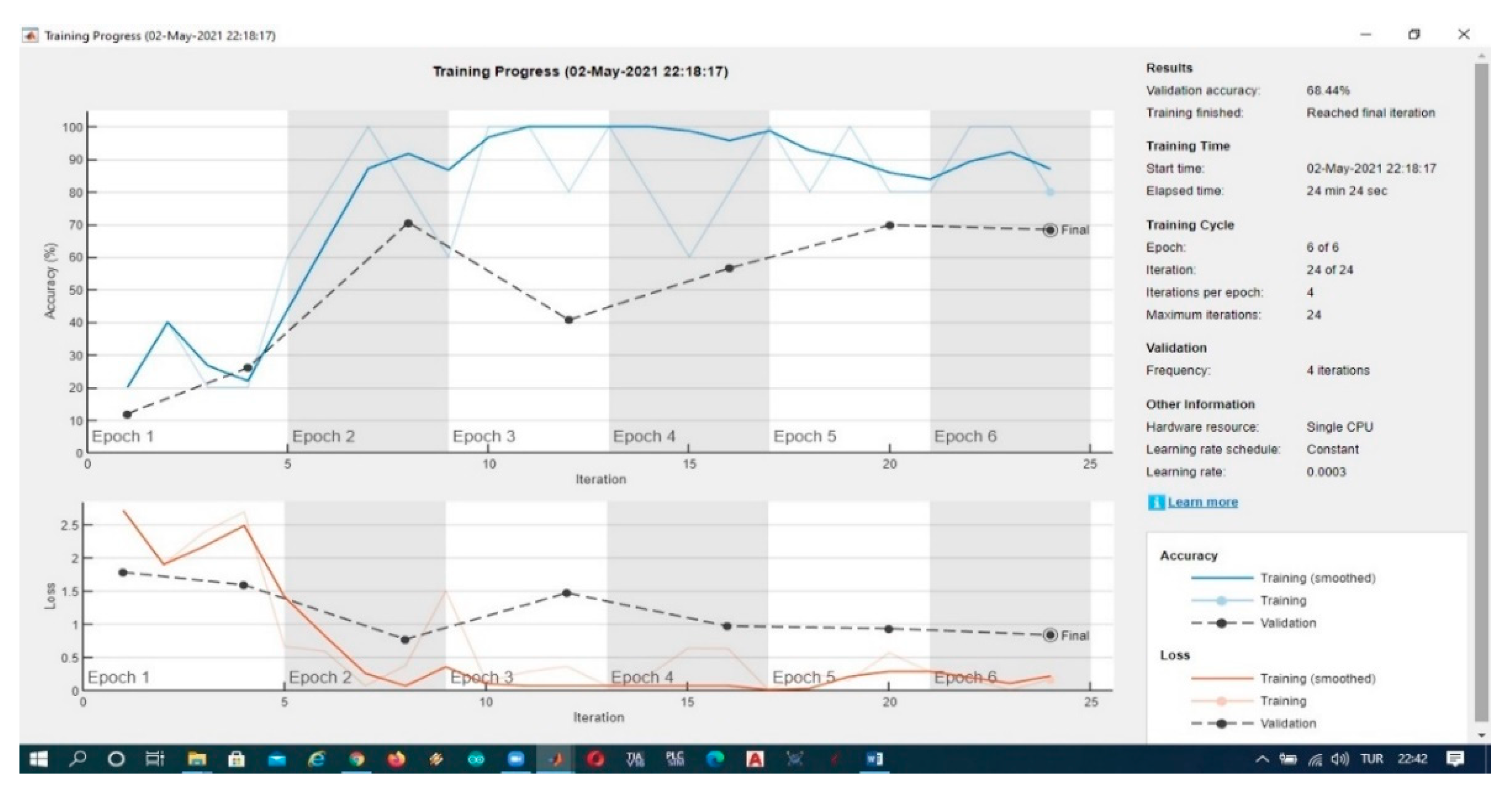
In VGGNet, the depth is 19 and there are 144 million parameters. VGGNet is greater than AlexNet in both depth and parameters. This is reflected in the rate of accuracy. The accuracy rate of VGGNet was 97.70%, approximately 2% higher than the accuracy rate of AlexNet. The training time in VGGNet was 961 min. Buddha was the longest training period. Figure 14 shows the training process of the GoogleNet architecture used in the system.

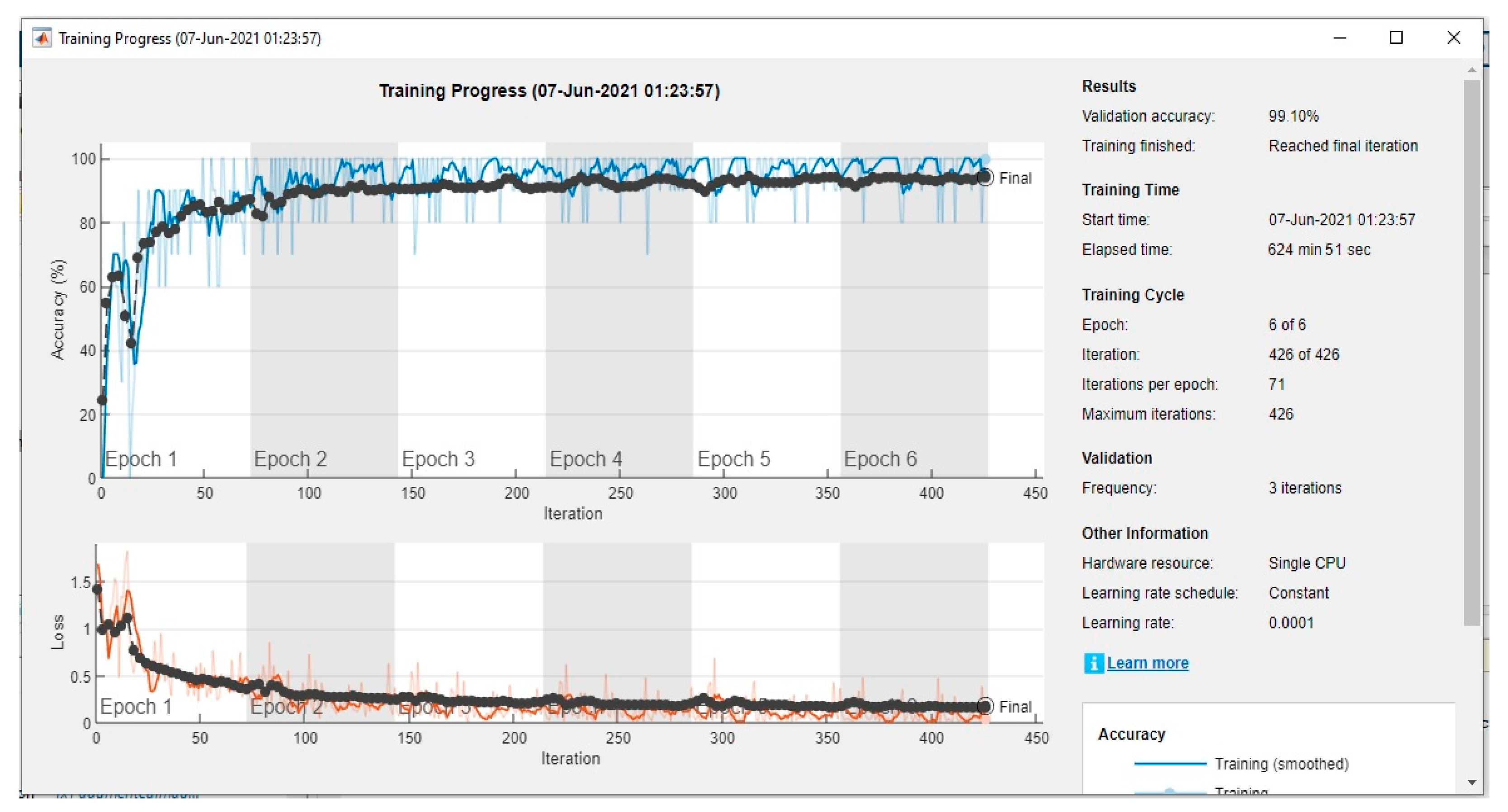
GoogleNet took had a training period of 24 min. The accuracy rate was the lowest, with 68.74%. It had a much higher error rate than normal people. Figure 15 shows the training process of the ResNet architecture used in the system.

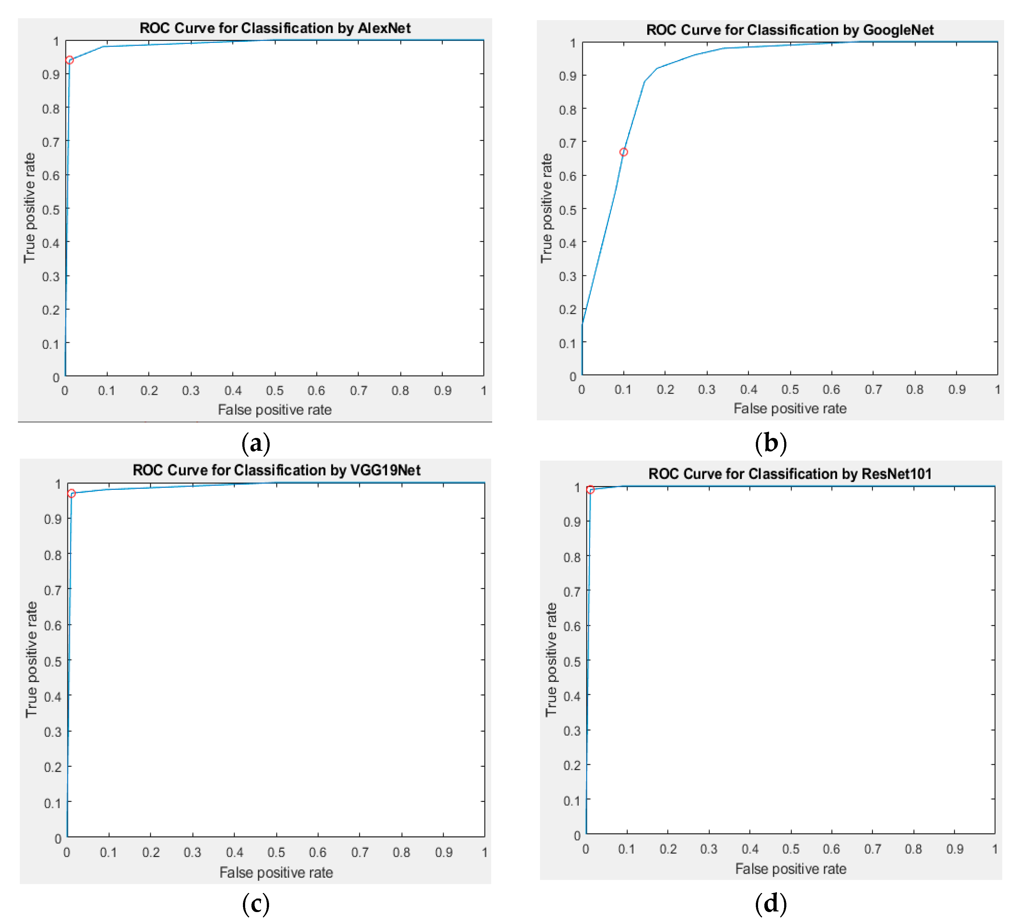
Nine different architectures were used in this study. Of these architectures, the learning outcomes of the AlexNet, GoogLeNet, VGGNet, and ResNet architectures are shown. The other architectures shown are versions with increased accuracy rates. The ROC curves of the four different architectures used have been calculated. Figure 16 shows ROC graphs belonging to four different architectures.

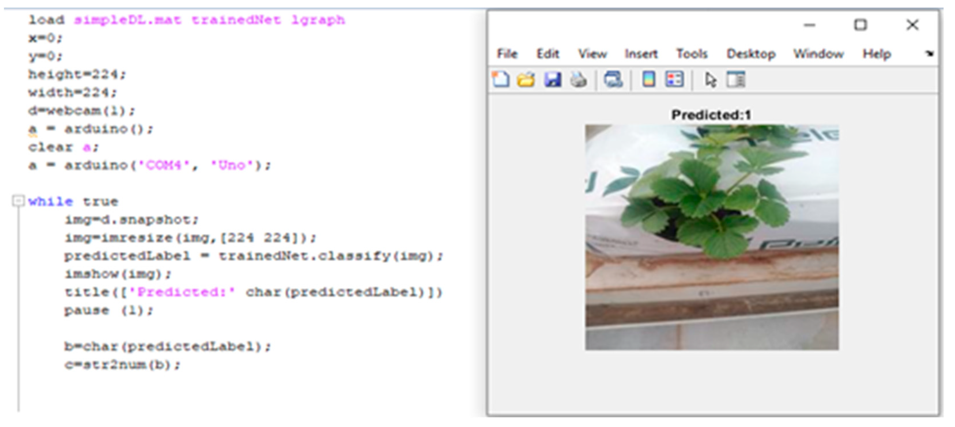
This study was performed in the program MATLAB. A picture was taken with the webcam and processed at 10:00 every morning. It worked with ResNet101 architecture in MATLAB for every process. Training was done with ResNet101 architecture. Testing was done with training files. The test program and program output are shown in Figure 17.

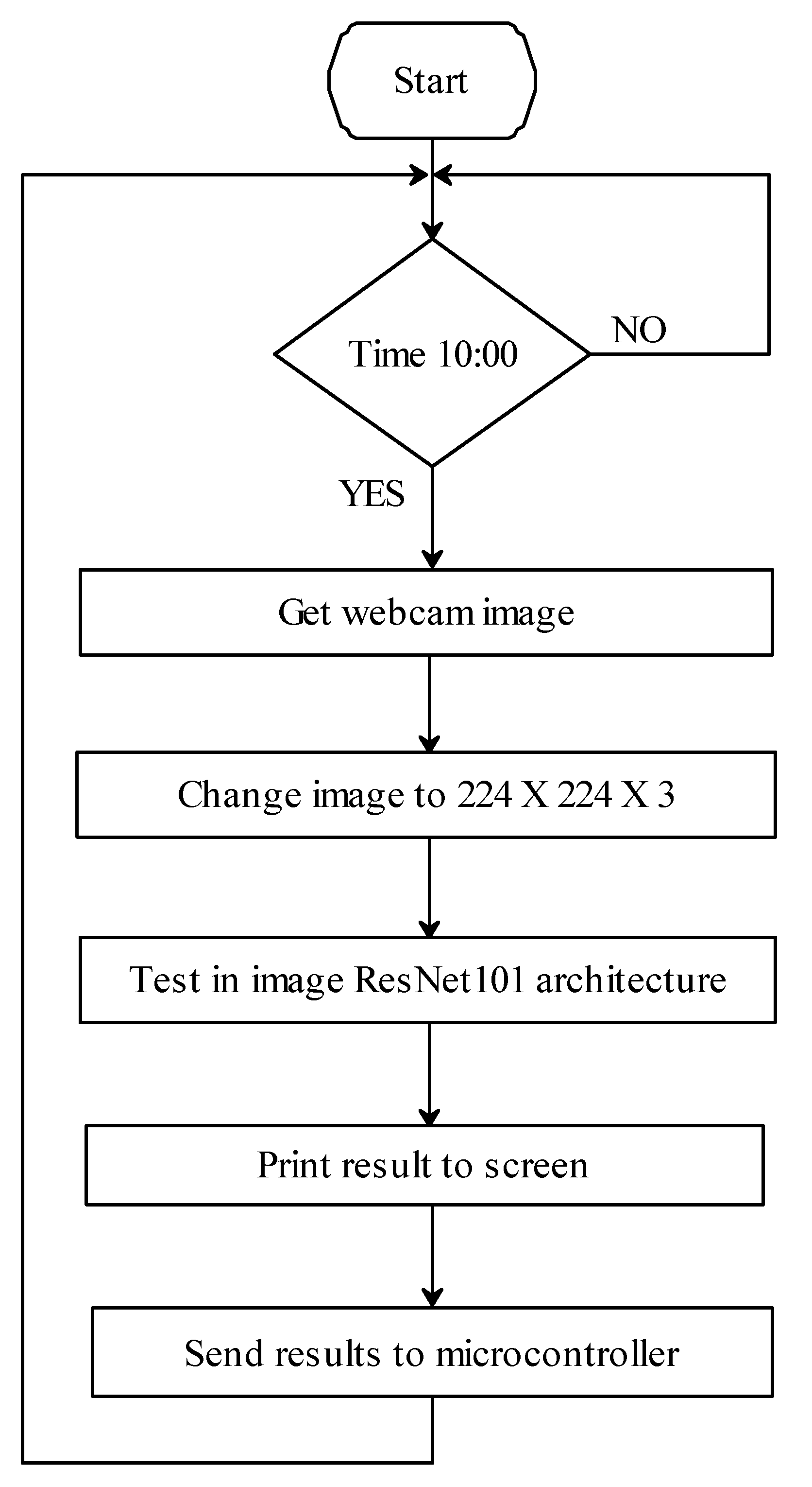
This study was carried out in the real-life environment of the plant. The photo of the plant was assessed at 10:00 every morning. The size of the captured image was first reduced. ResNet101 architecture, which gave the highest accuracy rate in the study, uses 224 × 224 photos as an input. After the size of the captured photo was reduced, the test process was carried out in the ResNet101 architecture. After the test process was finished, the result was obtained and the captured picture was shown on the computer screen. There was a USB connection between MATLAB and the microcontroller. The code for the microcontroller was written in MATLAB. After the test process was finished, the result was sent to the microcontroller. Figure 18 shows the test algorithm.

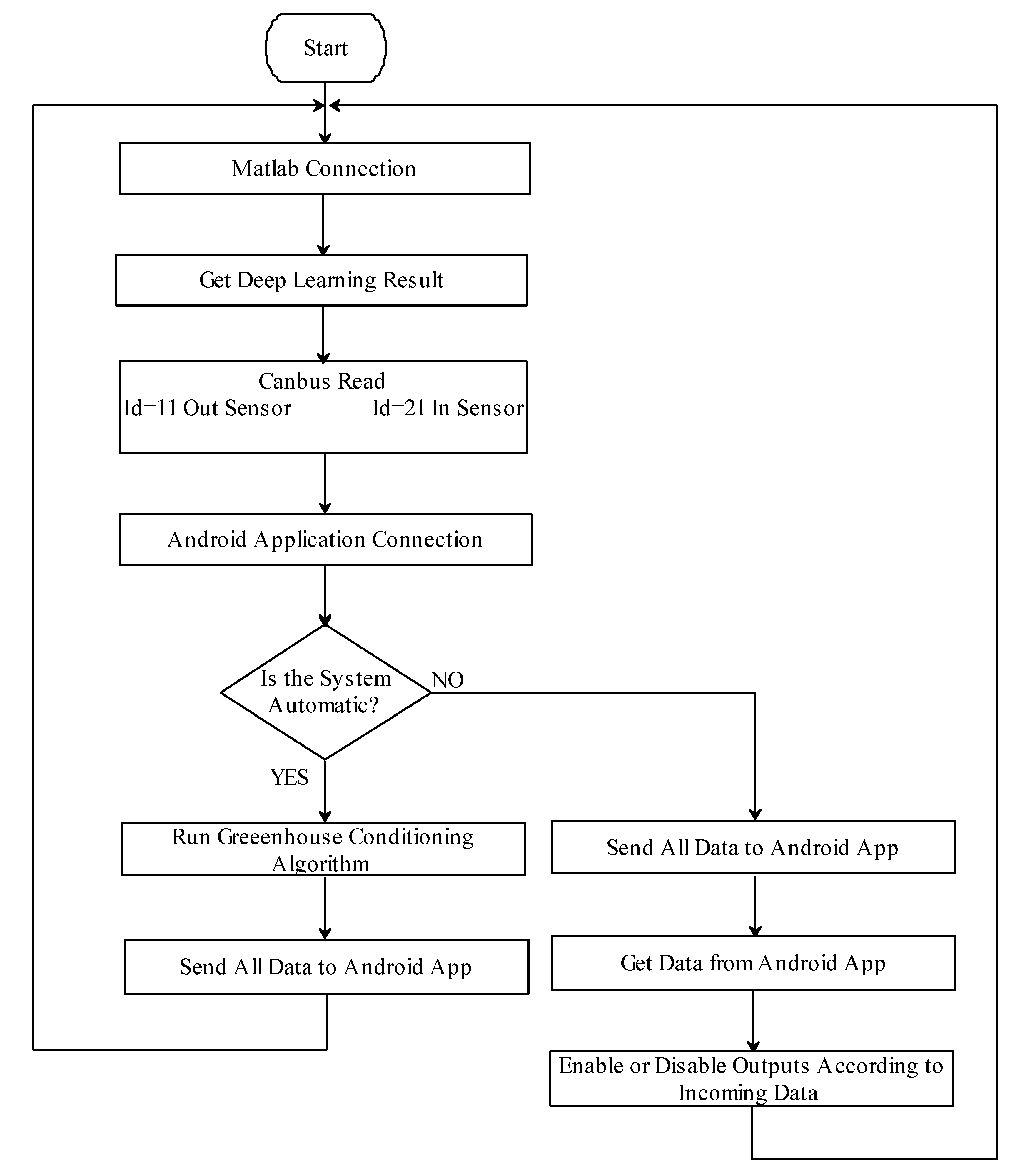
In this study, Canbus communication protocol was used for the communication of internal sensor, external sensor, irrigation, humidification, air conditioning, and the control part of the interface. Thanks to Canbus, communication was provided over long distances with less cables. All systems were connected via a single line with Canbus. Each system was given an ID number. Thus, the required system ID number can be easily found. In this study, 50 Kbit/sec was the preferred communication speed. In this way, data transmission was provided up to 1 km away. Figure 19 shows the general algorithm of the system.

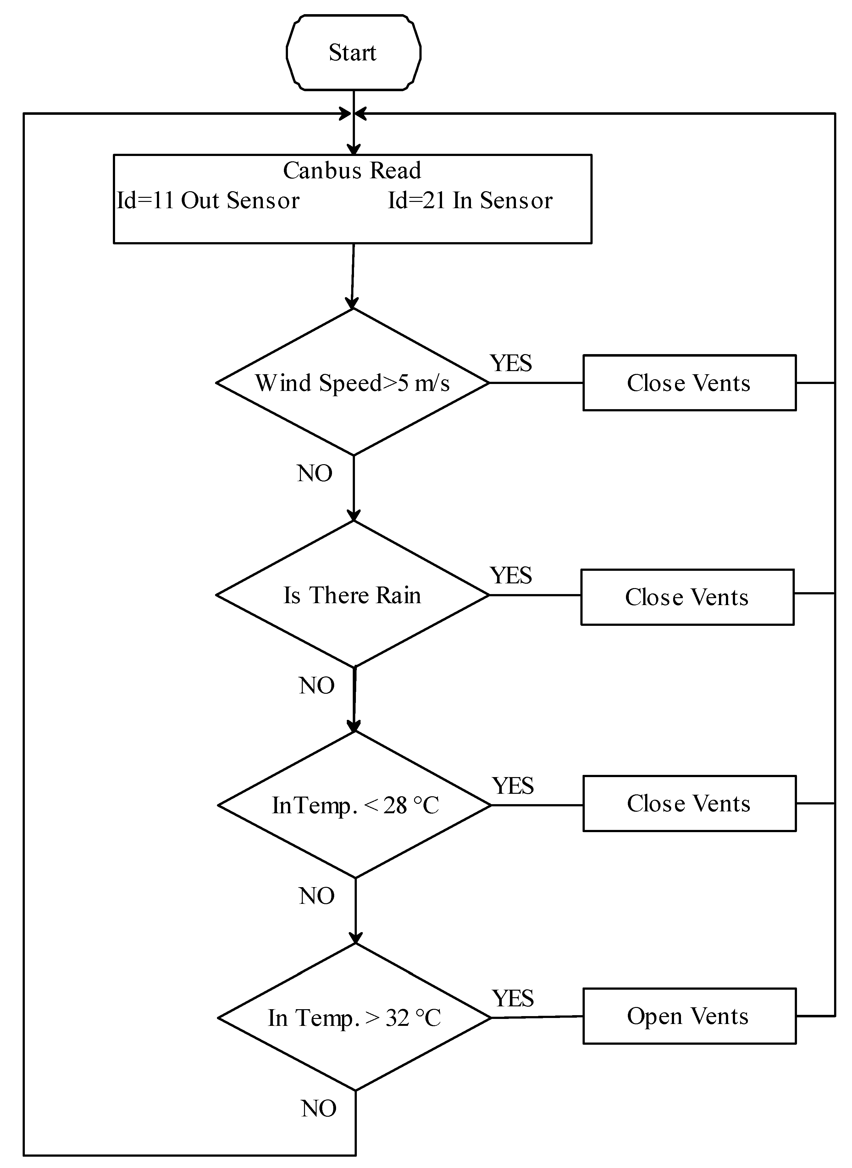
More than one algorithm was used in the study. Especially in automatic control, this was very important for the system to function by itself. The greenhouse air conditioning algorithm was designed to provide the ideal living environment for the plant. Figure 20 shows the indoor air conditioning algorithm.

The work carried out covers the entire process from the planting of the strawberry seedling to the end of the crop yield. During this process, the detection and treatment of diseases that may occur in the strawberry plants were carried out. For this reason, diseases that originated from five different strawberry plants were detected. At the same time, the determination of the three different life stages of the strawberry plant was carried out. This study was carried out while growing strawberry plants in the greenhouse.

One of the most important differences between this study and other studies in the literature is that this study was carried out in a real greenhouse, not in a laboratory environment. All procedures were performed while the strawberry plant was growing. For this, strawberry planting was carried out in a 16 m² greenhouse. Following this planting, every stage of the strawberry plant was photographed. The dataset was created from these photographs. This dataset was used by nine different deep learning architectures. The same dataset was used by each architecture. The architectures used, accuracy rates, and other data are shown in

Table 1. Algorithms used in the study.

Architecture Name	Image Input Size	Depth	Parameters	Training Time	Test Time	Accuracy Rate %
AlexNet	227 × 227	8	61 million	113 min	13.39 s	95.74
GoogleNet	224 × 224	22	7.0 million	24 min	7.56 s	68.44
ResNetInceptionV2	299 × 299	164	55.9 million	78 min	10.08 s	87.21
ResNetInceptionV3	299 × 299	48	23.9 million	151 min	8.53 s	93.77
ResNet18	224 × 224	18	11.7 million	426 min	7.55 s	97.05
ResNet50	224 × 224	50	25.6 million	553 min	8.54 s	94.75
ResNet101	224 × 224	101	44.6 million	878 min	9.57 s	99.80
VGG16Net	224 × 224	16	138 million	426 min	12.33 s	95.25
VGG19Net	224 × 224	19	144 million	113 min	13.58 s	97.70

.

Nine different algorithms were used in the study. Of the algorithms used, the ResNet101 architecture gave the highest accuracy rate. ResNet101 architecture had 99.80% accuracy, while a normal person had an error rate of 5–10%. An error rate that is less than human error was determined in this study. All algorithms were loaded with the same database. Although the photos in the database were the same, their sizes differed. Some algorithms used 224 × 224 photos, while others required 227 × 227 or 229 × 229 photos. For the training times, the highest training time was the SqueezeNet architecture, with 981 min. The lowest training time was GoogleNet, with 24 min. GoogleNet had the lowest training time but the highest error rate. The same computer was used for all training periods of the algorithms. Thus, the error rate arising from the system was minimized. Accuracy rates were not directly proportional to the training times. Thus, the parameters and depth of the algorithm were effective. Although SqueezeNet had the highest training time, the accuracy rate remained at 91.31%. Its 1.24 million parameters and 18 depths were far below those of the ResNet101 architecture.

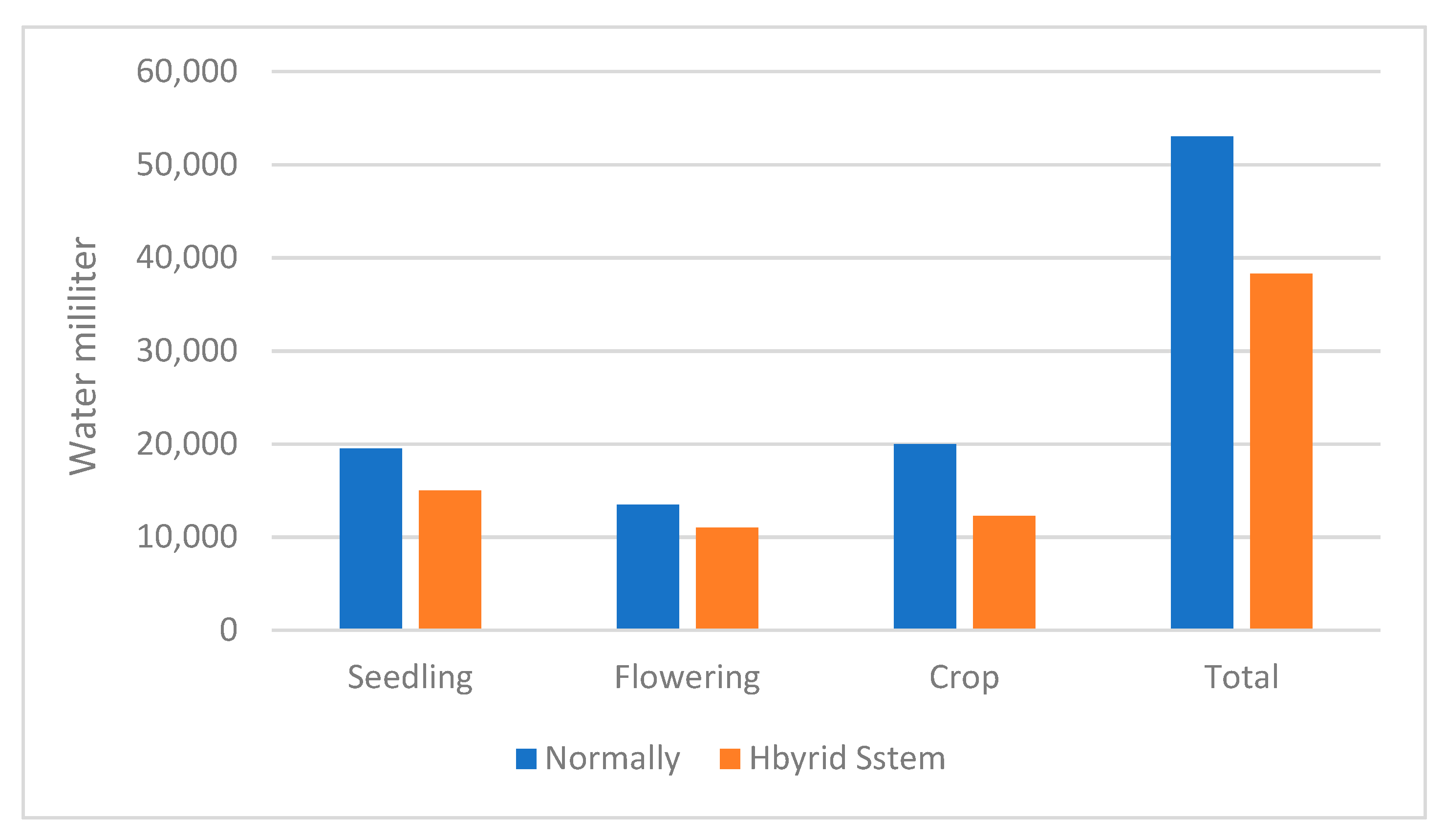
This study was carried out to increase the productivity of strawberry plants. With this in mind, a disease that can occur in the growth phase of the strawberry plant was determined. With this determination, the necessary chemical or chemical mixture was given to the plant and recovery was achieved as soon as possible. At the same time, three life stages of the plant—seedling, blooming, and crop—were determined. Between these stages of the strawberry plant, the climate needs to be adjusted. The sooner that the indoor air conditioning becomes suitable for the stage of the plant, the more that the efficiency will increase. In Figure 21, the efficiency of the system irrigated with the normal and the hybrid system is compared.

In addition to the outdoor temperature and humidity values, soil moisture was also measured in the irrigation system. Since the soil moisture was very low in the first seedling planting, the water yield was less. Afterwards, the water yield increased a lot.

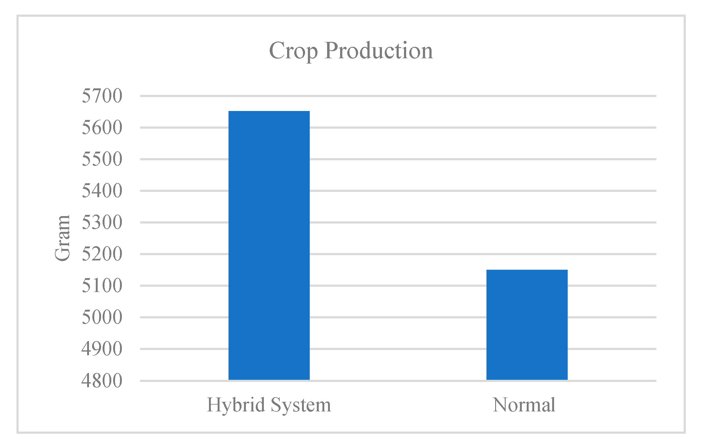
In this study, the strawberry plant grew very quickly. A total of 5652 g of crop was obtained in the plants grown with deep learning. A total of 5150 g of strawberry crop was obtained in the plants grown normally. This equates to 9.75% more product when using deep learning. Figure 22 shows a comparison of the strawberry production.

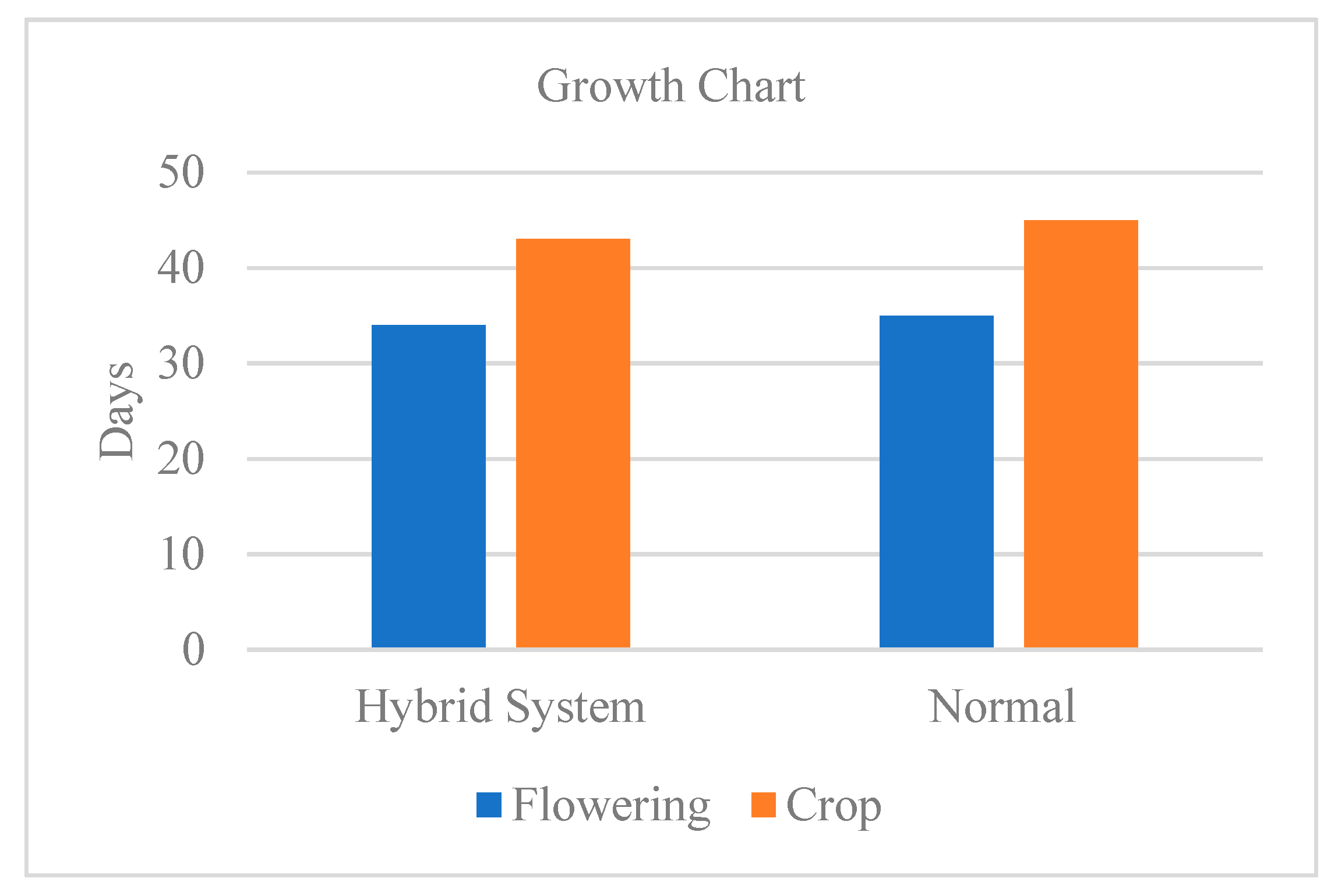
The strawberry plants grown with deep learning yielded more crops and were grown in a shorter time. In the plants that grew with deep learning, time to flowering was on average 2 days shorter. Crop giving was started 2 days earlier on average. Figure 23 comparison of the growth times of the strawberry plant.

4. Discussion

When the literature was examined, many studies have been carried out on disease detection with deep learning. These studies covered the leaf of the diseased plant. Then, all pictures were taken in a laboratory environment so that they were the same at the bottom. The datasets consisted of the taken photographs. These photographs were not taken in the real-life environment of the plant and did not cover the entire life cycle of the plant.

Table 2. Literature’s studies.

Authors	Architecture Name	Accuracy Rate %
Brahimi et al. [7]	AlexNet, GoogleNet	97.71
Rangarajan et al. [8]	AlexNet, VGG16	97.49
Khandelwal et al. [9]	GoogleNet	99.37
Waheed et al. [10]	Denset	9.,06
Espinosa et al. [11]	GoogleNet	70
Tang et al. [12]	ShuffleNet	99.14
Wang et al. [13]	Denset121, VGG16, ResNet50, MobileNet	90.02
Vasconeza et al. [20]	MobileNet, Inpection V2	93
Sajad et al. [21]	GoogleNet	9.05
Daobilige et al. [22]	Inception V3	95.48
Samyak et al. [23]	MobileNet	95.70
Yibin et al. [13]	Denset121, VGG16, ResNet50, MobileNet	90.02
Alkan et al. [24]	AlexNet, ResNet, GoogleNet	99.06
Ashwinkumar et al. [25]	MobileNet	98.50
Valeri et al. [26]	GoogleNet	99.72
Ben et al. [27]	VGG16	90
Cen et al. [28]	1D-CNN	9969
Xioa et al. [29]	MobileNet	98.,1
Paymode et al. [30]	VGG16	95.71
Anh et al. [31]	VGG16	91.8
Yuana et al. [32]	VGG16	98.15
Weng et al. [33]	SqueezeNet	99.71

shows the results of the studies in the literature.

When we looked at the literature, most studies used one or more architectures, but no more than five architectures were used. Ten different architectures were used in the study. Thus, a comparison was performed between ten architectures.

When the accuracy rates in the literature were examined, they varied according to the study. The most important factor in this study was the photos in the dataset. The closer the photos in the dataset were to the photo to be tested, the higher the accuracy. In order to increase the accuracy rate in this study, a trial sowing was conducted. Soilless agriculture cocopeat was used in this trial planting. The dataset was comprised of the photos taken during this trial planting. As a result, the later rate increased since the same cocopeat was in the photo in the recognition process of the disease. This study had the highest accuracy rate among the literature.

The studies in the literature have only taken one phase of the plant into account. This study covered the entire life cycle of the plant, the time elapsed from the plant’s seedling stage to its yielding.

This study was conducted to increase the productivity of strawberry plant. In this pursuit, a disease that may occur in the growth phase of the strawberry plant was determined. With this determination, the necessary chemical or chemical mixture was given to the plant and recovery was achieved as soon as possible. At the same time, three life stages of the plant—seedling time, blooming time, and crop time—were determined. Between these stages of the strawberry plant, the climate needs to be adjusted. The sooner the greenhouse air conditioning becomes suitable for the stage of the plant, the more that efficiency will increase.

5. Conclusions

In this study, five diseases and three healthy stages of strawberry plant were determined. This determination was conducted not only in the laboratory environment, but over the entire plant growing process in the greenhouse. Convolutional neural networks were used to perform the detection. In this study, the detection accuracy results were as follows: GoogleNet, 68.44%; InceptionResNetV2, 87.21%; InceptionV3, 93.77%; ResNet50, 94.75%; ResNet18, 97.05%; VGG16, 95.25%; AlexNet, 95.74%; VGG19, 97.70%; and ResNet101, 99.80%. In this study, fuzzy logic control was used to increase efficiency in water and humidity. As a result of the application of the deep learning system, 9.75% more crops were obtained. At the same time, the harvesting time was shortened by 4.75%. An efficiency increase of 8.51% was achieved in the irrigation system.