Application of Machine Learning to Express Measurement Uncertainty

Abstract

The continuing increase in data processing power in modern devices and the availability of a vast amount of data via the internet and the internet of things (sensors, monitoring systems, financial records, health records, social media, etc.) enabled the accelerated development of machine learning techniques. However, the collected data can be inconsistent, incomplete, and noisy, leading to a decreased confidence in data analysis. The paper proposes a novel “judgmental” approach to evaluating the measurement uncertainty of the machine learning model that implements the dropout additive regression trees algorithm. The considered method uses the procedure for expressing the type B measurement uncertainty and the maximal value of the empirical absolute loss function of the model. It is related to the testing and monitoring of power equipment and determining partial discharge location by the non-iterative, all-acoustic method. The example uses the dataset representing the correlation of the mean distance of partial discharge and acoustic sensors and the temperature coefficient of the sensitivity of the non-iterative algorithm. The dropout additive regression trees algorithm achieved the best performance based on the highest coefficient of determination value. Most of the model’s predictions (>97%) fell into the proposed standard measurement uncertainty interval for both “seen” and “unseen” data.

1. Introduction

The latest development of information and communication technologies in daily life enables more and more implementation of different devices and tools, their connectivity, and automatization of the work. Some of the essential characteristics of these systems are the generation of a large amount of data, various parameters’ monitoring and prediction, and the possibility to mitigate resource usage. To achieve the best results, artificial intelligence is used during the development of such platforms [1], but the evaluation of the measurement uncertainty of the applied models is also required.

The permanent increase in data processing power in modern devices and the availability of a vast amount of data via the internet and the internet of things (IoT) enabled the accelerated development of artificial intelligence (AI) methods. Given trends have actualized issues of AI hardware and algorithms’ energy efficiency and the possibility of optimal application of AI in real-time (autonomous cars, mobile phones, unmanned aerial vehicles, etc.). In addition to energy efficiency, current topics in the literature deal with the possibility of sudden outages, wrong decisions, sabotage and fraud, and optimal maintenance techniques for intelligent agents. In simpler terms, researchers are trying to answer the increasingly frequently asked question: “To what extent can intelligent agents be trusted?” There is no simple answer to this question because it involves the evaluation of intelligent agents (AI methods) in terms of transparency, controllability, availability, usability, resilience, reliability, accuracy, security, privacy, quality, etc. [2,3,4,5,6,7,8,9,10,11,12].

AI and machine learning (ML) techniques are used to analyze complex data and take proper actions. In modern society, various sectors that play vital roles, such as smart grids, intelligent transportation, cyber-security, and communication technologies, are supported by big data analysis and the effective use of AI and ML techniques [13,14,15,16]. The data collected from IoT (sensors, monitoring systems, financial records, health records, social media, etc.) can be inconsistent, incomplete, and noisy, leading to a decreased confidence in data analysis [17]. Controlling and quantifying ML models’ uncertainty improves data analysis’s reliability. It also enhances the belief in the model’s decisions.

An ML model consists of knowledge about model structure and training dataset. In the context of ML, the nature of uncertainty can be classified as epistemic (parameter uncertainty) and aleatoric (data uncertainty) [17,18,19,20]. In the literature, uncertainty quantification concepts relevant to ML are grouped as frequentist inference and Bayesian inference. Frequentist inference deals with errors in parameters’ estimates. Bayesian inference is used in traditional ML (Gaussian process regression (GPR), and GPR and physics-informed neural networks) and deep learning (Bayesian neural network and Bayesian physics informed neural network) [17,21]. These concepts primarily deal with model uncertainty [22,23,24] (inverse propagation problem) over measurement uncertainty [25]. Recently, researchers have had increased interest in quantifying the uncertainty related to ML models [26,27,28]. In the systematic literature reviews of ML and deep learning applications in smart cities [11], and the COVID-19 epidemic [12], the accuracy parameter received the most attention from the reviewed articles (28.1% and 48.8%, respectively). The number of research publications related to the topic has grown from around 7000 in 2011 to about 24,000 in 2020 [17].

The contributions of the research presented in the paper are:

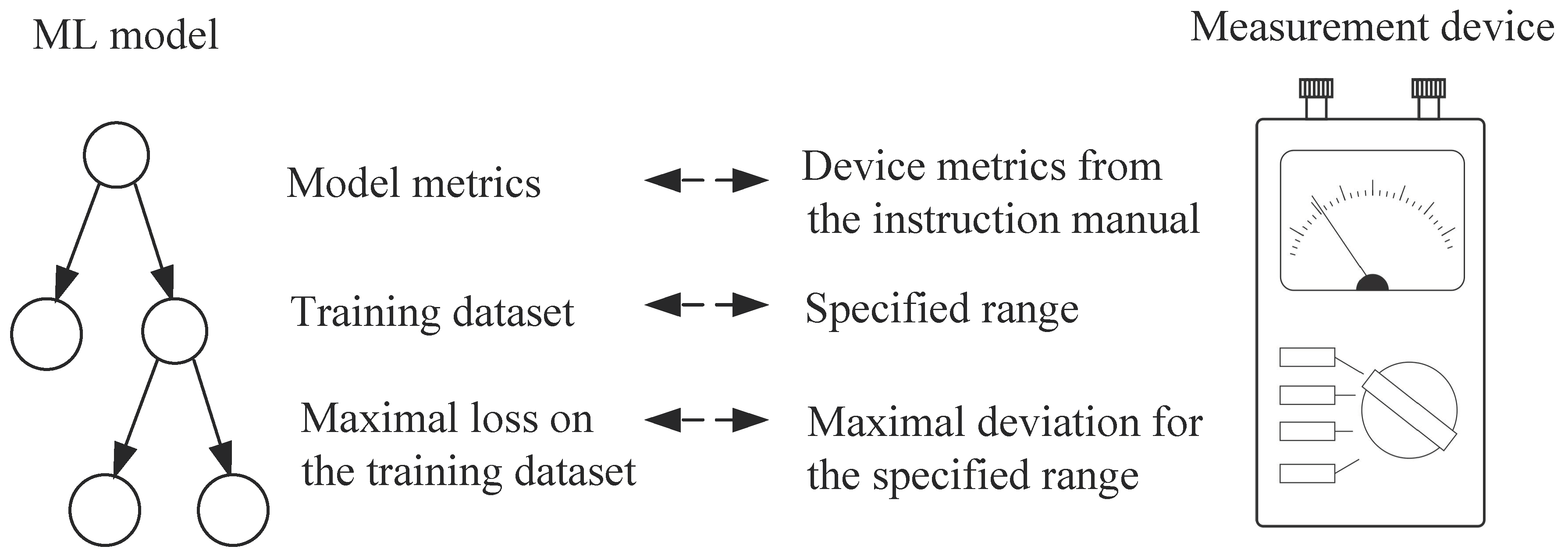
• To address the abovementioned issues, a novel “judgmental” [21] approach to evaluating the measurement uncertainty of the ML model is proposed. The method is based on the analogy of an ML model and an actual measurement device.
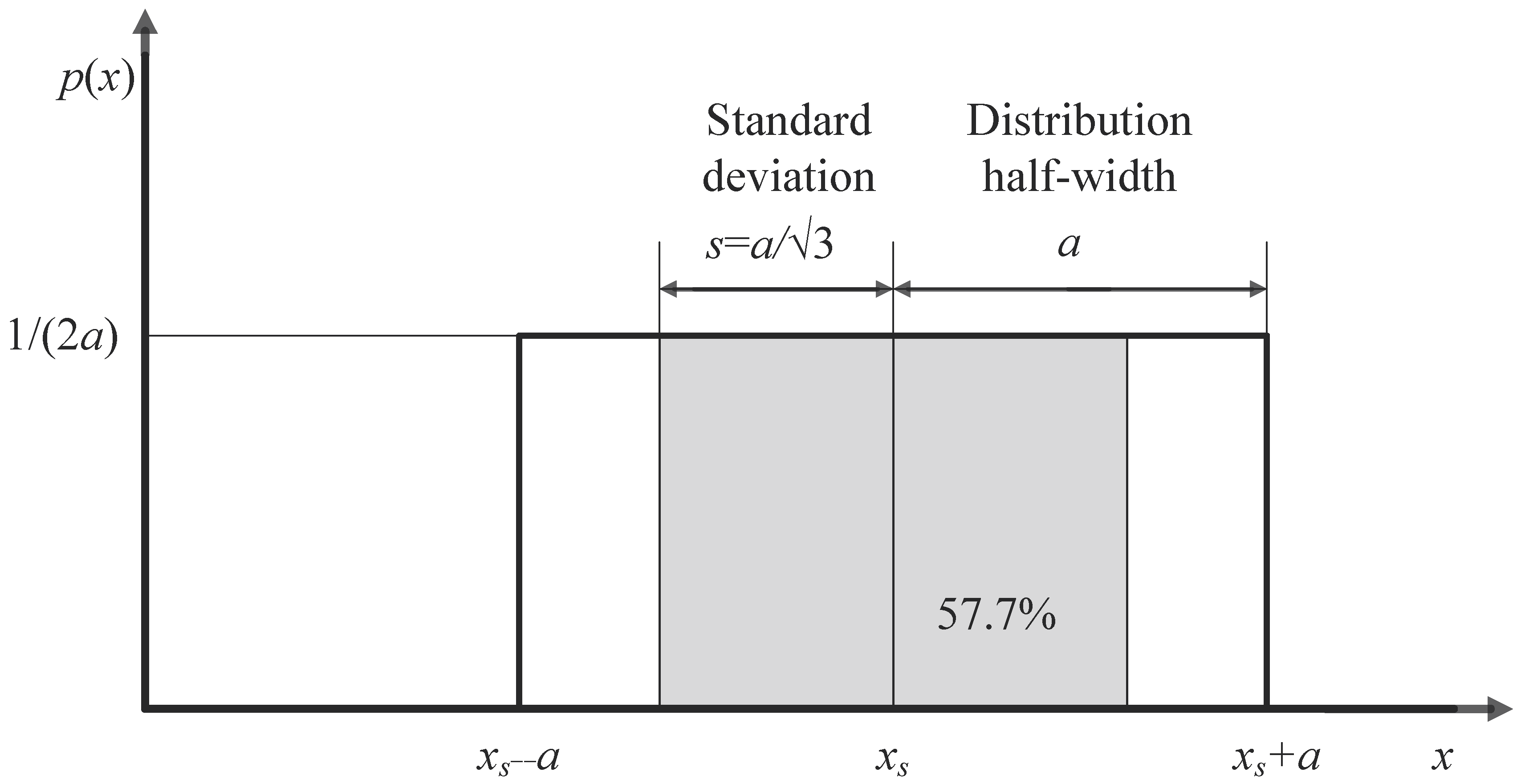
• It uses the procedure for expressing the type B measurement uncertainty [29] and the maximal value of the empirical absolute loss function of the ML model. Since expressing type B measurement uncertainty is based on the experience and judgment of the measurer, the approach is referred to as “judgmental [21]”.
• The considered ML model is related to the testing and monitoring of power equipment, i.e., determining the partial discharge (PD) location by the non-iterative, all-acoustic method [30,31].
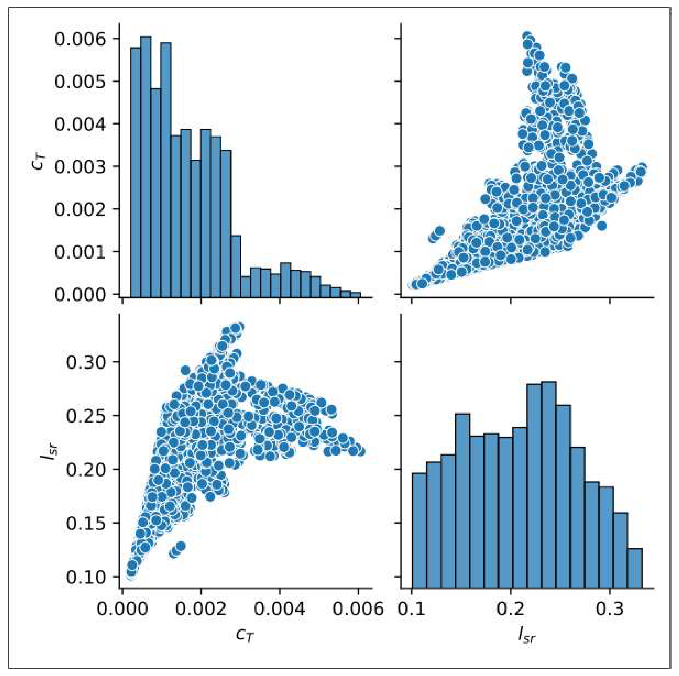
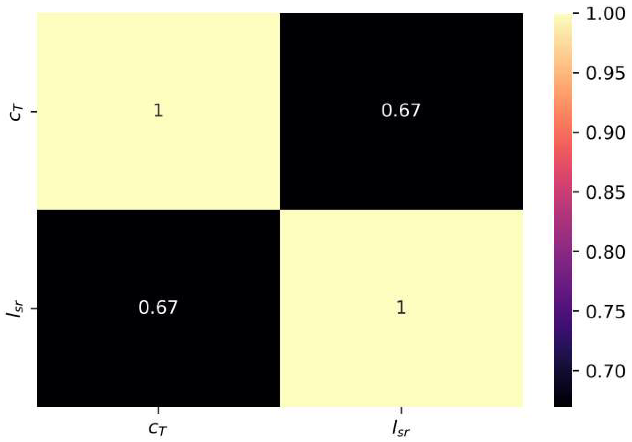
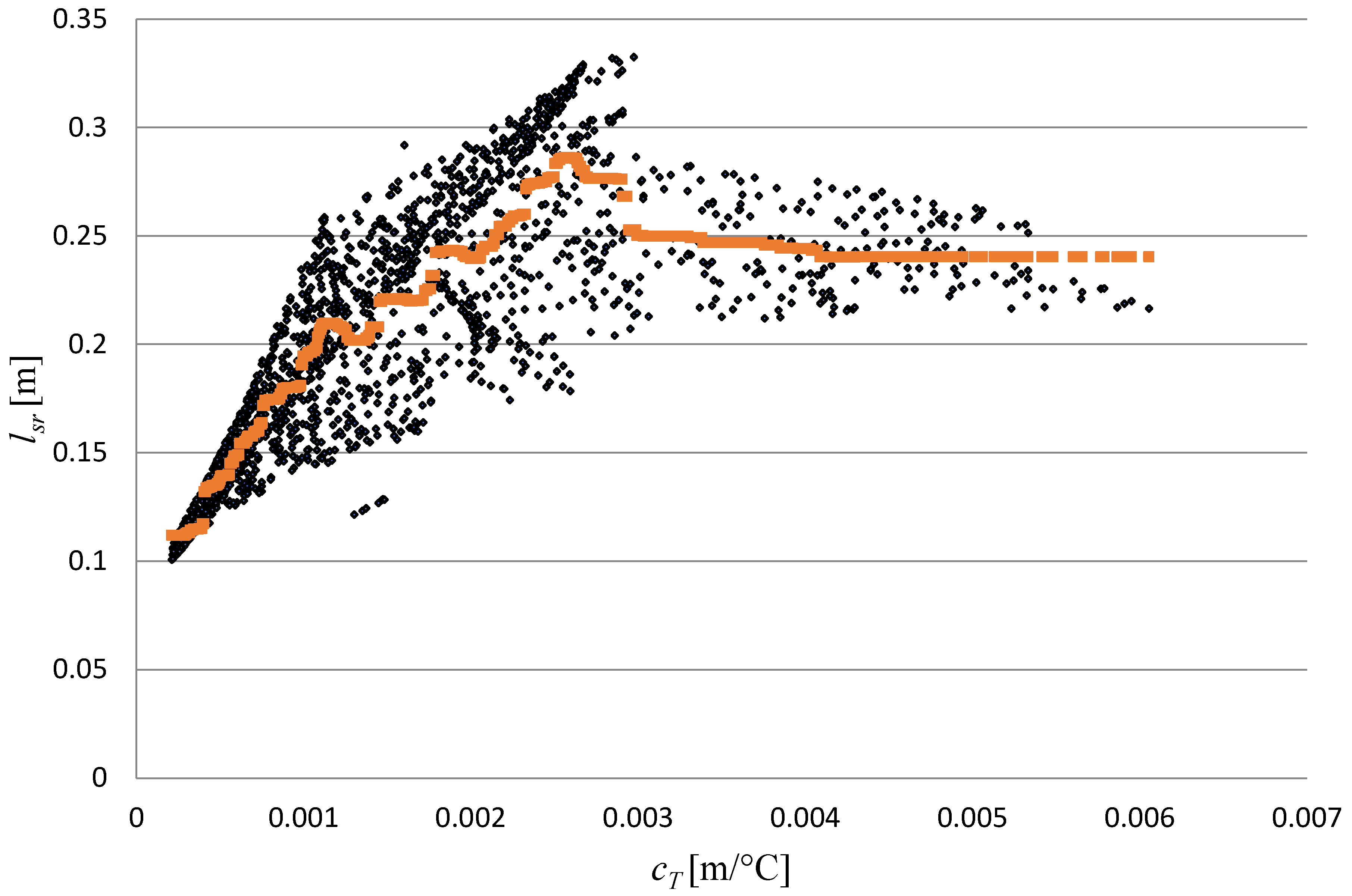
• The example uses the dataset representing the correlation of the mean distance of partial discharge and acoustic emission (AE) sensors and the temperature coefficient of sensitivity of the non-iterative algorithm [30].
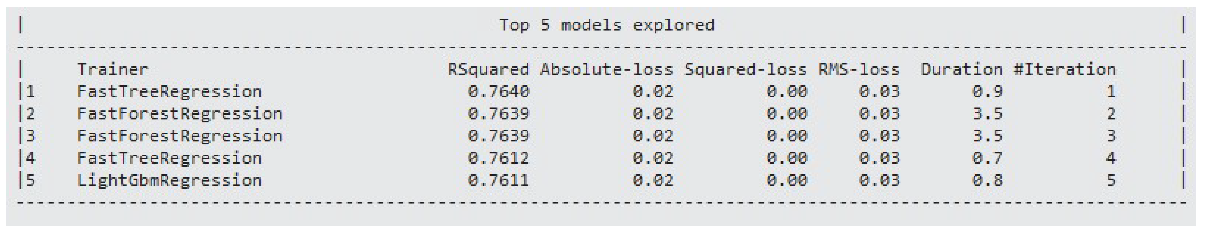
• Based on the highest coefficient of determination value, the dropout additive regression trees algorithm (DART) achieved the best performance.
• The proposed estimation procedure is not limited to the presented example but can also be used in all similar regression problems, including big data analysis.
• The proposed procedure is applicable even when the probability distribution of deviation of predicted values from correct values is unknown.

This paper consists of the following sections: Introduction; Methods; Experimental data, comparative analysis, and discussion; and Conclusion. The Methods section introduces measurement uncertainty, empirical loss function, a description of the DART algorithm, and the measurement uncertainty of the ML model. The following section explains the reasons for conducting the experiments and presents experimental results with appropriate analysis. Finally, the Conclusion provides deductions drawn from the results achieved in this study.

2. Methods

This section discusses measurement uncertainty, empirical loss function, description of the selected DART algorithm, and the ML model’s measurement uncertainty.

2.1. Measurement Uncertainty

It is impossible to determine the exact value of the measured quantity because the results of actual measurements contain a certain degree of uncertainty. Measurement error is the difference between the measured value and the “true value.” “True value” means a value measured by a reference standard, i.e., an available standard with the highest level of accuracy. The disadvantage of the given approach (error theory) in the processing and expressing measurement results is the absence of uniformity and the impossibility of comparing the same types of measurements from different institutions (researchers). To introduce standardization in the field of processing and expression of measurement results, the leading institutions of the international metrology system published the first version of the instructions for the expression of measurement uncertainty in 1993 [32].

When processing and expressing measurement results, it is necessary to determine three quantities: measurement result, measurement uncertainty, and statistical certainty. The measurement result is the mean value of repeated measurements (x_s). Measurement uncertainty (dispersion or scattering of measurement results) is expressed as an interval around the mean value in which the actual value of the measured quantity is expected to be found. The degree of statistical certainty (probability) is added to the given data.

The standard measurement uncertainty u is equal to the standard deviation s. Depending on the associated probability distribution, the statistical certainty corresponding to the x_s ± u interval is approximately 57.7% for the uniform distribution, 65% for the triangular distribution, 68% for the normal distribution [33], etc.

The standard combined measurement uncertainty u_c is calculated if several components influence the measurement uncertainty. The extent to which the corresponding components affect the combined measurement uncertainty can be expressed with sensitivity coefficients [32]:

$$u_c=\sqrt{{\left(\frac{\partial y}{\partial x_1}\right)}^2{u_{x_1}}^2+{\left(\frac{\partial y}{\partial x_2}\right)}^2{u_{x_2}}^2+\dots +{\left(\frac{\partial y}{\partial x_k}\right)}^2{u_{x_k}}^2},$$

(1)

$$c_i=\frac{\partial y}{\partial x_i},i=1\dots k,$$

(2)

$$u_c=\sqrt{{c_1}^2{u_{x_1}}^2+{c_2}^2{u_{x_2}}^2+\dots +{c_k}^2{u_{x_k}}^2}.$$

(3)

The value c_i is the sensitivity coefficient of the influential quantity x_i. The given coefficient expresses a measure of the influence of the corresponding component on the combined measurement uncertainty.

The expanded measurement uncertainty U is the product of the standard measurement uncertainty and the coverage factor (k). The coverage factor has values in the interval from √3 to 3. The coverage factor depends on the associated distribution function and the target statistical certainty (for example, for the normal distribution, a coverage factor of exactly two corresponds to a statistical confidence of approximately 95%, a coverage factor of 2.56 corresponds to a statistical confidence of approximately 99%, and a coverage factor of 3 corresponds to a statistical confidence of approximately 99.7%) [32,33].

Based on the determination methodology, there are two basic types of measurement uncertainty: type A and type B. The normal distribution is usually associated with type A measurement uncertainty, while type B measurement uncertainty is related to various distributions [32].

Type B measurement uncertainty is determined by all methods other than the statistical analysis of repeated measurement results. Considering that the set of methods for determining type B measurement uncertainty is not defined, the choice of procedures depends on the requirements, knowledge, and experience of the measurer. The given measurement uncertainty can also be specified in the case when the measurement was performed only once.

Sources of information on type B measurement uncertainty can be data on the operational measurement procedure, data on the measuring equipment (manufacturer’s instructions, calibration certificates), knowledge about the influence of the environment on the measurement process (temperature, humidity), knowledge about the impact of disturbances (electromagnetic, mechanical), results of previous measurements, variability of personnel performing the same type of measurement, etc. The standard measurement uncertainty of type B, u_B, is equal to the standard deviation due to the influence of the quantity from which it originates. In most cases, due to the lack of data, the measurement uncertainty of type B has an assumed uniform distribution [32,33,34].

In uniform distribution, the values of the measurement results belong to the limited interval (x_s − a, x_s + a). All values within the interval have an equal probability, i.e., p(x) = 1/(2a), where a is the half-width of the distribution. The standard deviation is s = a/√3, where approximately 57.7% of the measurement results are in the interval (x_s − s, x_s + s) (Figure 1). The given distribution is applied when there is insufficient information about the measurement instrument [33].

The result of the measurement uncertainty calculation should be presented transparently, i.e., in such a way as to show all the relevant facts related to the procedure of determining the measurement uncertainty. The tabular representation of the given data is called the measurement uncertainty budget. The data in the measurement uncertainty budget are significant measurement quantities, their distribution functions with standard measurement uncertainties, appropriate coverage factors, etc. [33].

2.2. Empirical Loss Function

Expressing utility in machine learning is standard using a loss function L. The loss function is defined as the amount lost utility by predicting h(x) = $\widehat{y}$ when correct is the answer f(x) = y [1]:

$$L(y,\widehat{y})=Utility(y)-Utility(\widehat{y}).$$

(4)

In general, minor deviations are better than larger ones. The two functions that follow the previously mentioned logic are the absolute value of the difference (L₁ loss) and the square of the difference (L₂ loss) [1]:

$$\begin{array}{cc}{L}_1(y,\widehat{y})=\left|y-\widehat{y}\right|,& L_2(y,\widehat{y})={(y-\widehat{y})}^2.\end{array}$$

(5)

Theoretically, an agent can maximize its expected utility by choosing the hypothesis that minimizes the expected loss of overall input–output pairs it considers. An agent can estimate the generalization loss for a hypothesis h (to a loss function L) with an empirical loss on a set E of N examples (average loss) [1]:

$$EmpLos{s}_{L,E}(h)=\frac{1}{N}{\displaystyle \sum _{(x,y)\in E}L(y,\widehat{y})}.$$

(6)

Instead of average loss, the maximal loss can be used [35]:

$$EmpLos{s}_{L,E}(h)=\underset{(x,y)\in E}{\max }L(y,\widehat{y}).$$

(7)

In the given cases, the estimated best hypothesis from the set of hypotheses H is the one with the minimum empirical loss [1]:

$${\widehat{h}}^{*}=\underset{h\in H}{\arg \min } EmpLos{s}_{L,E}(h).$$

(8)

Minimizing average loss is a more popular approach. In some situations, researchers recommend minimizing maximal loss instead [35].

Empirical average loss with L₂ function is usually called Mean Square Error (MSE) [36]:

$$MSE=EmpLos{s}_{L_2,E}(h)=\frac{1}{N}{\displaystyle \sum _{(x,y)\in E}{(y-\widehat{y})}^2}.$$

(9)

If the MSE is observed as the variance of the function y, then the MSE represents the variance of hypothesis h.

Another way of evaluating the generalization of the hypothesis mentioned in the literature is quantifying the progress achieved by learning (h) to some trivial predictive method that is available even without training. One such trivial approach is to take the mean value of the output on some set of examples and use that value for prediction (generalization). The given method is simple and does not consider the input value when predicting in contrast to the hypothesis obtained by training [37].

The coefficient of determination, or R², compares the mean squared errors of the hypothesis h and the mean value of the output (variance) for the observed N examples [37]:

$$R^2=1-\frac{MSE}{\mathrm{var}[y]}=1-\frac{{\displaystyle \sum _{i=1}^N{(y-\widehat{y})}^2}}{{\displaystyle \sum _{i=1}^N{(y-\overline{y})}^2}}.$$

(10)

2.3. DART Algorithm

Ensemble training algorithms achieve high accuracy for numerous machine learning tasks. For ensembles to achieve better accuracy than the individual hypotheses from which they are composed, the hypotheses should be with uncorrelated errors. While some classes of ensemble training algorithms such as random forests independently add each hypothesis to the set, algorithms using boosting such as AdaBoost and Multiple Additive Regression Trees (MART) [38] incrementally add hypotheses. This technique increases the ensemble’s accuracy by reducing the sensitivity to specific features or cases that may exist in individual hypotheses.

Boosting algorithms add hypotheses focused on improving the current set of hypotheses, which is achieved by modifying the training problem between iterations. Although this guarantees that the added hypothesis differs from the set, the new hypotheses usually focus on a small subset of the problem and thus have no significant prediction of the original problem. This increases the risk of adding hypotheses that fit too well to specific cases. It is a well-known problem in boost training and in the MART algorithm that uses ensemble training by boosting regression decision trees. In a given algorithm, trees added in later iterations tend to affect the prediction of only a few hypotheses and make a negligible contribution to the prediction of all remaining hypotheses. In turn, this can negatively affect the algorithm’s performance on new data by increasing the capacity of the set without significantly improving its training error. Additionally, this makes the set hypersensitive to the contributions of a few initially added trees. This issue of posterior trees affecting the prediction of only a tiny fraction of hypotheses is referred to as over-specialization.

The most common approach to combat over-specialization in the MART algorithm is reduction. Here, the contribution of each new tree is reduced by a constant value called the reduction factor. Downscaling helps to reduce the influence of the first trees; however, as the size of the set increases, the problem of over-specialization reappears.

In the Dropout Additive Regression Trees (DART) algorithm [39], which is based on the MART algorithm, a different approach is proposed to solve the issue of over-specialization. This approach involves dropout, a technique proposed in the context of regularizing deep neural networks. In neural networks, dropout is used to silence a random portion of the neural connections during the training process. This method has significantly contributed to the success of deep neural networks for many tasks, including, for example, object classification in images.

The DART algorithm introduces a new way of using dropout for a set of decision trees: complete tree silencing instead of feature silencing. In the available literature, evaluation results of the DART algorithm on three different tasks, ranking, regression, and classification, using publicly available large-scale datasets, show that DART outperforms MART and random forest in each task by significant margins [39]. One of the reasons for the improved performance of the DART algorithm is that it addresses the issue of over-specialization and results in a more balanced contribution of all trees in the hypothesis set.

Another place where DART differs from MART is the addition of a new tree to the set where DART performs the normalization step. To ensure that the impact of the omitted trees and the newly added tree remains the same as the impact of the omitted trees before adding the new tree to the set, the newly added tree is first scaled by 1/k and then together with the omitted trees by k/k + 1. The number k represents the number of omitted trees in a given iteration step of the algorithm.

The DART algorithm reduces the problem of over-specialization. Therefore, it can be seen as regularization, where the number of omitted trees controls the degree of regularization. If no tree is left out, DART is no different from the MART algorithm. If all trees are omitted, DART is indistinguishable from a random forest. Therefore, the size of the omitted set allows the DART algorithm to vary between an “aggressive” MART to a “conservative” random forest.

2.4. Measurement Uncertainty of ML Model

In supervised learning, the training set consists of input–output pairs. The given set can be viewed as if a corresponding output value was measured for each input value. Generally speaking (without noise), one input corresponds to one output. The original output values from the training set can be considered the exact values, while the values obtained by the ML model are the measured values. Since only one output value is measured for one input value, it is impossible to express the measurement uncertainty of type A. However, it is possible to express the measurement uncertainty of type B because only one measurement is needed.

One of the common sources for determining type B measurement uncertainty is the measurement instrument manufacturer’s instructions. It contains the maximum errors determined by the manufacturer for specific ranges of the measured quantity. The analogy with the ML model would be the maximal L₁ loss on the training dataset (Figure 2).

Assuming the uniform distribution, the standard type B measurement uncertainty of the ML model is equal to standard deviation s:

$$u=\sqrt{u_A^2+u_B^2}=u_B=s=\frac{\underset{(x,y)\in E}{\max }{L}_1(y,\widehat{y})}{\sqrt{3}},$$

(11)

with the degree of statistical certainty of 57.7%.

Additional sources of type B measurement uncertainty mentioned in Section 2.1 and analytically presented in [29] can also find an analogy with the ML model. For example, uncertainty due to the measurement’s device indication (scale) reading by the operator can be analogous to taking a lower number of significant digits or inadequate rounding of predicted values by the ML model. The ML models are executed on appropriate hardware that optionally observes the environment through actuators. The CPU calculation uncertainty, the actuator measurement uncertainty, etc., can also be additional sources of type B measurement uncertainty of the ML model. These additional sources were not considered in the study.

3. Experimental Data, Comparative Analysis, and Discussion

The considered experiment is related to testing and monitoring of power equipment, i.e., determining PD location in the mineral oil by the non-iterative, all-acoustic method. The non-iterative algorithm gives a solution for a system of nonlinear equations describing PD location. The algorithm has 19 parameters (16 inputs and 3 outputs), i.e., a relatively sizeable nineteen-dimensional state space. The location of PD is determined indirectly. All of the parameters, both input and output, can influence the combined measurement uncertainty of the non-iterative algorithm [30].

The correlation between the two input parameters of the algorithm, the mean distance of PD and AE sensors, and the temperature coefficient of sensitivity was observed in [30]. The correlation was expressed via the mean values of the parameters. Calculating the mean value of the parameter does not consider the value on which it depends. The mean values were calculated using the Monte Carlo (MC) method, which was time-consuming. Additionally, not all possible values were generated through MC randomization.

To overcome the mentioned shortcomings, supervised learning technique is proposed. The dataset generated through MC randomization is used as a training dataset of a model that can subsequently predict even the “unseen” data. The chosen metric for ranking the models’ performance is R². The R² compares the model’s hypothesis variances and the label’s mean value from the training dataset. In this way, the improvement over the existing calculation of the mean value of the parameter can be directly evaluated.

The tradeoff of this approach is the appearance of additional uncertainty generated by the ML model. The tradeoff can be made more acceptable by quantifying and controlling the given uncertainty by the procedure proposed in Section 2.4.

3.1. Experimental Data and Comparative Analysis

As mentioned in the previous section, the training dataset has one input parameter (feature) and one output parameter (label). The mean distance between PD and AE sensors l_sr is the predicted value, while the temperature coefficient of sensitivity c_T is the feature. The dataset originated from [30] and was generated using MC simulation. The number of MC simulations was 10,000. In the simulations, a cube-shaped area filled with mineral oil with a side length of 0.60 m was considered. The PD location was unchanged (0.05 m, 0.54 m, 0.14 m) while the sensors’ positions were randomized. The temperature coefficient of sensitivity was calculated using maximum change in the result for detecting the location of PD ∆gmax and mineral oil’s temperature change ∆T, c_T = ∆gmax/∆T. The considered data is for the mineral oil’s temperature range of 40 °C [30]. The dataset’s characteristics are visualized in Figure 3 and Figure 4, while its basic statistical properties are given in

Table 1. Basic statistical characteristics of the employed dataset.

Count	1799	1799
	cT[m/°C]	lsr[m]
Average value	0.001691	0.2083
Standard deviation	0.001168	0.0580
Minimum	0.000213	0.1008
25%	0.000778	0.1594
50%	0.001450	0.2132
75%	0.002324	0.2516
Maximum	0.006055	0.3325

. The dataset employed in this study can be retrieved from the following URL: https://doi.org/10.6084/m9.figshare.20401953.v1 (accessed on 23 August 2022).

A free, open-source, cross-platform framework, ML.NET is used to train the ML model. The ML.NET framework offers multiple machine learning algorithms. The framework can iteratively train multiple algorithms and rank them according to the appropriate performance metrics. A ranked list of the best training algorithms (top five) is suggested to the user. Several different classes (trainers) are available for solving regression problems, grouped into trainers for linear regression and binary logistic regression [40].

The development tool was Microsoft Visual Studio Community 2019. The training time was 120 s on a 64-bit Windows 10 PC with an Intel Core i7-8750H processor and 16 GB of RAM. The results of the training are presented in Figure 5.

The trainers were ranked based on the value of R². The FastTreeRegression trainer that implements the DART algorithm (R² = 0.7666) achieved the best result. The second best was the FastForestRegression trainer that implements the random forest algorithm (R² = 0.7658). The predictions of the model that implements the DART algorithm are presented in Figure 6.

To calculate the measurement uncertainty of the model using the expression (11), it is necessary to calculate the maximal L₁ loss on the considered dataset. The ML.NET does not include this metric in the output results, so it was calculated additionally. The maximal L₁ loss of the model on the considered dataset was 0.1078 m.

Assuming the discrete uniform distribution, the model’s standard type B measurement uncertainty is u_B = 0.06 m with a degree of statistical certainty of 57.7%. The number of predictions that did not fall into the standard measurement uncertainty interval was 53, i.e., 2.9%. Additionally, the expanded uncertainty was calculated. It used the coverage factor of √3, U_B ≈ 0.11 m, with the degree of statistical certainty of 100%.

The previous training session used all input–output pairs; i.e., all the data were “seen” by the model. The next session used 90% of the input–output pairs (Figure 7). The 10% (180) randomly picked input–output pairs were used to evaluate the calculated standard measurement uncertainty.

The maximal L₁ loss of the model trained on 90% of the dataset was 0.1060 m, i.e., u_B = 0.06 m. The model was used for predictions in the 10% dataset. The number of predictions that did not fall into the standard measurement uncertainty interval in the 10% “unseen” dataset was five, i.e., 2.7%, similar to the previous session.

3.2. Discussion

The used ML model that implements the DART algorithm to predict the value of the l_sr contributed to the uncertainty budget of the non-iterative algorithm by u = u_B = 0.06 m (

Table 2. The example of the row layout in the measurement uncertainty budget of a non-iterative algorithm would correspond to the use of the ML model to estimate l_sr.

Quantity	Estimate	Standard Uncertainty	Probability Distribution	Sensitivity Coefficient	Uncertainty Contribution
lsr	Predicted value by the ML model	0.06 m	Uniform	1.0	0.06 m

). The improvement to the trivial calculation of the mean value of l_sr was between four and five times (R² > 0.75). The DART algorithm performed better than the random forest, which was expected. The results showed that most predictions (>97%) fell into the standard measurement uncertainty interval for both the whole considered dataset and the 10% “unseen” dataset.

The cube-shaped area with a side length of 0.60 m was considered in the experiment. In the case of standard measurement uncertainty of the ML model, the contribution to the uncertainty budget of the non-iterative algorithm accounts for 10% of the side length value, while expanded measurement uncertainty accounts for approximately 18%.

The statistical value of >97% for the standard uncertainty of the ML model can find its usefulness only when put in the appropriate context. For example, the standard measurement uncertainty can be used for the periodical testing of power equipment performed on demand or annually. On the other hand, for the online monitoring of power equipment where the number of PD occurrences and temperature oscillations in mineral oil can be very high, the expanded measurement uncertainty of the ML model could be more appropriate to use as a contribution to the measurement uncertainty budget of a non-iterative algorithm.

4. Conclusions

In this paper, the authors presented a novel “judgmental” approach to evaluating the measurement uncertainty of the machine learning model that implements the DART algorithm. The considered method uses the procedure for expressing the type B measurement uncertainty and the maximal value of the empirical absolute loss function of the model. It is related to the testing and monitoring of power equipment and determining partial discharge location by the non-iterative, all-acoustic method. The example uses the dataset representing the correlation of the mean distance of partial discharge and acoustic sensors and the temperature coefficient of sensitivity of the non-iterative algorithm.

The proposed procedure for uncertainty expression is straightforward and uncomplicated to implement. The results showed that most predictions (>97%) fell into the standard measurement uncertainty interval for both “seen” and “unseen” data. The advantage of employing the type B measurement uncertainty is that it uses the available data without needing additional optimization (even one input–output pair is sufficient).

The limitation of the proposed method is that it is applicable only in supervised learning regression techniques. Additionally, the method did not consider other sources of the type B measurement uncertainty of the ML model, such as inadequate rounding of predicted values by the ML model, CPU calculation uncertainty, actuator measurement uncertainty, etc.

Further research will focus on applying the proposed procedure in various situations and datasets.

References

- Russell, S.; Norvig, P. Artificial Intelligence: A Modern Approach, 3rd ed.; Prentice Hall: Hoboken, NJ, USA, 2010. [Google Scholar]
- Chellappa, R.; Theodoridis, S.; van Schaik, A. Advances in Machine Learning and Deep Neural Networks. Proc. IEEE 2021, 109, 607–611. [Google Scholar] [CrossRef]
- Yu, K.; Tan, L.; Mumtaz, S.; Al-Rubaye, S.; Al-Dulaimi, A.; Bashir, A.K.; Khan, F.A. Securing Critical Infrastructures: Deep-Learning-Based Threat Detection in IIoT. IEEE Commun. Mag. 2021, 59, 76–82. [Google Scholar] [CrossRef]
- Louridas, P.; Ebert, C. Machine Learning. IEEE Softw. 2016, 33, 110–115. [Google Scholar] [CrossRef]
- Benkhelifa, E.; Welsh, T.; Hamouda, W. A Critical Review of Practices and Challenges in Intrusion Detection Systems for IoT: Toward Universal and Resilient Systems. IEEE Commun. Surv. Tutor. 2018, 20, 3496–3509. [Google Scholar] [CrossRef]
- Shinde, P.P.; Shah, S. A Review of Machine Learning and Deep Learning Applications. In Proceedings of the 4th International Conference on Computing, Communication Control and Automation (ICCUBEA), Pune, India, 16–18 August 2018. [Google Scholar]
- Al-Turjman, F.; Zahmatkesh, H.; Shahroze, R. An overview of security and privacy in smart cities’ IoT communications. Trans. Emerg. Telecommun. Technol. 2022, 33, e3677. [Google Scholar] [CrossRef]
- Ahmed, M.; Cox, D.; Simpson, B.; Aloufi, A. ECU-IoFT: A Dataset for Analysing Cyber-Attacks on Internet of Flying Things. Appl. Sci. 2022, 12, 1990. [Google Scholar] [CrossRef]
- Fagbola, F.I.; Venter, H.S. Smart Digital Forensic Readiness Model for Shadow IoT Devices. Appl. Sci. 2022, 12, 730. [Google Scholar] [CrossRef]
- Ashfaq, Z.; Mumtaz, R.; Rafay, A.; Zaidi, S.M.H.; Saleem, H.; Mumtaz, S.; Shahid, A.; De Poorter, E.; Moerman, I. Embedded AI-Based Digi-Healthcare. Appl. Sci. 2022, 12, 519. [Google Scholar] [CrossRef]
- Heidari, A.; Navimipour, N.J.; Unal, M. Applications of ML/DL in the management of smart cities and societies based on new trends in information technologies: A systematic literature review. Sustain. Cities Soc. 2022, 85, 104089. [Google Scholar] [CrossRef]
- Heidari, A.; Navimipour, N.J.; Unal, M.; Toumaj, S. The COVID-19 epidemic analysis and diagnosis using deep learning: A systematic literature review and future directions. Comput. Biol. Med. 2022, 141, 105141. [Google Scholar] [CrossRef] [PubMed]
- Ullah, Z.; Al-Turjman, F.; Mostarda, L.; Gagliardi, R. Applications of Artificial Intelligence and Machine learning in smart cities. Comput. Commun. 2020, 154, 313–323. [Google Scholar] [CrossRef]
- Hariri, R.H.; Fredericks, E.M.; Bowers, K.M. Uncertainty in big data analytics: Survey, opportunities and challenges. J. Big Data 2019, 6, 44. [Google Scholar] [CrossRef]
- Sarker, I.H. Machine Learning: Algorithms, Real-World Applications and Research Directions. SN Comput. Sci. 2021, 2, 160. [Google Scholar] [CrossRef]
- Shende, M.K.; Salih, S.Q.; Bokde, N.D.; Scholz, M.; Oudah, A.Y.; Yaseen, Z.M. Natural Time Series Parameters Forecasting: Validation of the Pattern-Sequence-Based Forecasting (PSF) Algorithm; A New Python Package. Appl. Sci. 2022, 12, 6194. [Google Scholar] [CrossRef]
- Siddique, T.; Mahmud, M.S.; Keesee, A.M.; Ngwira, C.M.; Connor, H. A Survey of Uncertainty Quantification in Machine Learning for Space Weather Prediction. Geosciences 2022, 12, 27. [Google Scholar] [CrossRef]
- Walker, W.E.; Harremoës, P.; Rotmans, J.; van der Sluijs, J.P.; Van Asselt, M.; Janssen, P.; Von Krauss, M.K. Defining Uncertainty: A Conceptual Basis for Uncertainty Management in Model-Based Decision Support. Integr. Assess. 2003, 4, 5–17. [Google Scholar] [CrossRef]
- Siddique, T.; Mahmud, M.S. Classification of fNIRS Data Under Uncertainty: A Bayesian Neural Network Approach. In Proceedings of the IEEE International Conference on E-health Networking, Application & Services (HEALTHCOM), Shenzhen, China, 1–2 March 2021; IEEE: Piscataway, NJ, USA, 2021; pp. 1–4. [Google Scholar]
- Van Asselt, M.; Rotmans, J. Uncertainty in integrated assessment modelling. Clim. Chang. 2002, 54, 75–105. [Google Scholar] [CrossRef]
- Cox, M.; O’Hagan, A. Meaningful expression of uncertainty in measurement. Accredit. Qual. Assur. 2022, 27, 19–37. [Google Scholar] [CrossRef]
- Yu, D.; Wu, J.; Wang, W.; Gu, B. Optimal performance of hybrid energy system in the presence of electrical and heat storage systems under uncertainties using stochastic p-robust optimization technique. Sustain. Cities Soc. 2022, 83, 103935. [Google Scholar] [CrossRef]
- Fangjie, G.; Jianwei, G.; Yi, Z.; Ningbo, H.; Haoyu, W. Community decision-makers’ choice of multi-objective scheduling strategy for integrated energy considering multiple uncertainties and demand response. Sustain. Cities Soc. 2022, 83, 103945. [Google Scholar] [CrossRef]
- Yan, Q.; Lin, H.; Li, J.; Ai, X.; Shi, M.; Zhang, M.; Gejirifu, D. Many-objective charging optimization for electric vehicles considering demand response and multi-uncertainties based on Markov chain and information gap decision theory. Sustain. Cities Soc. 2022, 78, 103652. [Google Scholar] [CrossRef]
- Volodina, V.; Challenor, P. The importance of uncertainty quantification in model reproducibility. Philos. Trans. R. Soc. A Math. Phys. Eng. Sci. 2021, 379, 20200071. [Google Scholar] [CrossRef]
- Levi, D.; Gispan, L.; Giladi, N.; Fetaya, E. Evaluating and Calibrating Uncertainty Prediction in Regression Tasks. Sensors 2022, 22, 5540. [Google Scholar] [CrossRef] [PubMed]
- Pires, C.; Barandas, M.; Fernandes, L.; Folgado, D.; Gamboa, H. Towards Knowledge Uncertainty Estimation for Open Set Recognition. Mach. Learn. Knowl. Extr. 2020, 2, 505–532. [Google Scholar] [CrossRef]
- Fotis, G.; Vita, V.; Ekonomou, L. Machine Learning Techniques for the Prediction of the Magnetic and Electric Field of Electrostatic Discharges. Electronics 2022, 11, 1858. [Google Scholar] [CrossRef]
- Fotis, G.; Vita, V.; Maris, T.I. Rise Time and Peak Current Measurement of ESD Current from Air Discharges with Uncertainty Calculation. Electronics 2022, 11, 2507. [Google Scholar] [CrossRef]
- Polužanski, V.; Kartalović, N.; Nikolić, B. Impact of Power Transformer Oil-Temperature on the Measurement Uncertainty of All-Acoustic Non-Iterative Partial Discharge Location. Materials 2021, 14, 1385. [Google Scholar] [CrossRef]
- Besharatifard, H.; Hasanzadeh, S.; Heydarian-Forushani, E.; Alhelou, H.H.; Siano, P. Detection and Analysis of Partial Discharges in Oil-Immersed Power Transformers Using Low-Cost Acoustic Sensors. Appl. Sci. 2022, 12, 3010. [Google Scholar] [CrossRef]
- ISO. Guide to the Expression of Uncertainty in Measuremen; ISO: Geneva, Switzerland, 2008. [Google Scholar]
- European Accreditation. EA-4/02 M (2013): Evaluation of the Uncertainty of Measurement in Calibration; European Accreditation: Geneva, Switzerland, 2013. [Google Scholar]
- Singapore Accreditation Council. Guidance Notes EL 001: Guidelines on the Evaluation and Expression of Measurement Uncertainty for Electrical Testing Field; Singapore Accreditation Council: Singapore, 2019.
- Shalev-Shwartz, S.; Wexler, Y. Minimizing the Maximal Loss: How and Why? arXiv 2016, arXiv:1602.01690. [Google Scholar]
- Wang, Q.; Ma, Y.; Zhao, K.; Tian, Y. A Comprehensive Survey of Loss Functions in Machine Learning. Ann. Data Sci. 2022, 9, 187–212. [Google Scholar] [CrossRef]
- Chicco, D.; Warrens, M.J.; Jurman, G. The coefficient of determination R-squared is more informative than SMAPE, MAE, MAPE, MSE and RMSE in regression analysis evaluation. PeerJ Comput. Sci. 2021, 7, e623. [Google Scholar] [CrossRef] [PubMed]
- Friedman, J.H.; Meulman, J.J. Multiple additive regression trees with application in epidemiology. Stat. Med. 2003, 22, 1365–1381. [Google Scholar] [CrossRef] [PubMed]
- Rashmi, K.V.; Gilad-Bachrach, R. DART: Dropouts meet Multiple Additive Regression Trees. arXiv 2015, arXiv:1505.01866. [Google Scholar]
- Ahmed, Z.; Amizadeh, S.; Bilenko, M.; Carr, R.; Chin, W.-S.; Dekel, Y.; Dupre, X.; Eskarveskiy, V.; Filipi, S.; Finley, T.; et al. Machine learning at microsoft with ML.Net. In Proceedings of the ACM SIGKDD International Conference on Knowledge Discovery and Data Mining, Anchorage, AK, USA, 4–8 August 2019. [Google Scholar]