Article

Research on the Dynamic Damage Properties and Determination of the Holmquist–Johnson–Cook Model Parameters for Sandstone

1
School of Mechanics and Civil Engineering, China University of Mining and Technology-Beijing, Beijing 100083, China
2
State Key Laboratory of Simulation and Regulation of Water Cycle in River Basin, China Institute of Water Resources and Hydropower Research, Beijing 100048, China
*
Author to whom correspondence should be addressed.
Appl. Sci. 2022, 12(16), 8366; https://doi.org/10.3390/app12168366
Submission received: 18 July 2022 / Revised: 16 August 2022 / Accepted: 17 August 2022 / Published: 21 August 2022
(This article belongs to the Special Issue Multiphysics Modeling for Fracture and Fragmentation of Geomaterials)

1. Introduction

The drilling and blasting method is efficient, economical and reliable in many engineering construction projects, such as in tunnel excavation [1], mining [2] and damming [3]. The study of rock dynamics under an impact load is an important problem [4]. The dynamic mechanical properties of rock materials are quite different from the static properties, so the response of rock materials under impact loading is a hot issue in rock dynamics [5]. Stimulated by engineering practice, the testers have become increasingly modern and intelligent, which provides scientific and effective research methods for the study of the mechanical properties of the rock dynamics [6,7]. The split Hopkinson pressure bar (SHPB), invented in 1949, has been extensively used to determine a material’s dynamic performance [7,8,9,10]. The application of the SHPB on rocks was first reported by Hauser [11], in which a rock stress–strain curve was derived. Subsequently, scholars have conducted many valuable studies using the SHPB, such as compressive strength and tensile strength studies [12,13].
It is worth noting that only some of the energy from explosives is used to break rocks during blasting engineering construction, and the rest acts on the surrounding rock. The surrounding rock may experience deformation, instability, collapse and other accidents. The main reason is that although the stress wave generated by a single blast may not damage the surrounding rock in the middle and far areas, the primary joints of the rock mass will expand and gradually penetrate under the effect of multiple low amplitude stress waves and finally failure will occur [14]. This is a process of cumulative damage of the rock mass, which is characterized by the deterioration of the mechanical properties and reductions in bearing capacity and stability. Therefore, it is of great practical significance to study the damage characteristics of rocks under impact loading, especially the cumulative damage evolution law under multiple stress waves [15]. Although scholars have conducted many studies on the dynamic mechanical properties of rocks, there are only few studies on the damage behavior of rocks under repeated impact loading. Zhu et al. [16] found that the damage of sandstone occurred near the dynamic peak stress, and subsequently the internal cracks of the rock entered the development stage. Wu et al. [17] and Luo et al. [18] performed dynamic damage studies on granite and leptynite using a modified SHPB. They found that the P-wave velocity and axial strain gradually deteriorated with repeated impacts. Li et al. [19] conducted repeated impact tests on granite and found that the cumulative damage depended on the peak stress of the dynamic load with a fixed duration. Jin et al. [20,21] carried out repeated impact tests by using an SHPB system with axial and confining pressures and established a damage evolution model of sandstone. Li et al. [22,23] studied the dynamic characteristics of green sandstone subjected to repeated impacts and reported that the initiation of new cracks and the elongation of existing cracks were the main mechanisms for the degradation of the sandstone under repeated impacts. However, the dynamic damage evolution law, damage threshold and failure pattern of rocks have rarely been studied. Therefore, it is urgent to improve the understanding of the dynamic damage behaviors of rocks subjected to repeated impacts.
Meanwhile, the study of the dynamic constitutive model of rock materials is helpful to further analyze the dynamic mechanical and damage behaviors under different stress conditions. Currently, the common constitutive models for rock dynamics include the Holmquist–Johnson–Cook (HJC) model [24], the Riedel–Hiermaier–Thoma (RHT) model [25] and the Johnson–Holmquist (JH) model series [26]. All three of these models consider the high strain rate, large strain and nonlinear high pressure and softening due to material damage under impact loading. The HJC model was proposed for the computation of concrete subjected to high strain, a high strain rate and high stress, where a set of parameters for normal concrete was given. The RHT model was proposed based on the JH model to make up for the shortcomings of the HJC model, where the third deviatoric stress invariants (J3) are ignored. However, the application of the RHT model is largely restricted owing to the need to determine its 34 parameters. The HJC model is an excellent constitutive model and reflects both a material’s viscous and elastic–plastic characteristics. Scholars have used the HJC model to simulate and study the dynamic mechanical properties of rock materials [27,28], but they have not proposed a set of test methods for determining the parameters of specific rocks. More importantly, the default parameters recommended by the model or the corresponding parameters of concrete of a certain strength grade have been adopted. Therefore, more efforts should be made to propose a set of test methods for determining the parameters of the HJC model for specific rocks.
Although scholars have conducted extensive research on the dynamic mechanical properties of rock materials, there are few studies on the cumulative damage and regularity of the failure pattern evolution of sandstone under impact loads. Moreover, the research on the dynamic constitutive model of rock materials lags behind that of the static constitutive model, and the establishment of a dynamic constitutive model is far less abundant than that of rocks under static loads. In the study presented in this paper, the dynamic mechanical properties, damage evolution law and failure pattern of sandstone under the effect of stress waves are studied by using the SHPB test system. On this basis, a set of methods for systematically determining the sandstone parameters of the HJC model is proposed. Finally, the correctness of the parameter values is verified by simulating the SHPB test. The research results can provide theoretical support for the stability evaluation and seismic performance evaluation of the surrounding rock in tunnel excavation, mining and other engineering operations.

2. Experimental Setup

2.1. Rock Specimens

The sandstone materials were obtained from a quarry in Sichuan, China. In our experiments, cylindrical specimens were extracted by coring the same rock block, which was of good quality. The rock cores were processed into two specimens with dimensions of Φ50 mm × 100 mm and Φ50 mm × 40 mm, as suggested by the International Society for Rock Mechanics (ISRM) [29], which were used to perform the static and dynamic tests, respectively. Two ends of the specimen were ground to be flat to 0.02 mm tolerance and not depart from perpendicularity to its axis by more than 0.001 rad. The side surface of the specimen was smooth, free of abrupt irregularities and straight to within 0.02 mm. The specimens were homogeneous, with the following properties: density ρ = 2.61 g/cm3, P-wave speed Cs = 3291 m/s, elastic modulus E = 25.60 GPa, Poisson’s ratio v = 0.22, uniaxial compressive strength σc = 76.13 MPa, uniaxial tensile strength σt = 7.63 MPa.

2.2. SHPB System

The impact experiments were conducted using the SHPB system at China University of Mining and Technology, Beijing, and the schematic and physical map of the experimental setup are shown in Figure 1. The SHPB bar system consists of a striker, an incident bar, a transmitted bar and an absorbing bar. The striker and bars are made of high-strength Al alloys with an elastic wave velocity of 5090 m/s, which share a maximum diameter of 50 mm. The striker with a length of 400 mm launched by the gas gun impacts the incident bar to generate a compressive wave, which propagates through the specimen and afterwards to the transmitted bar. The strains induced by the wave on the bars are measured by two sets of strain gauges attached on the incident and transmitted bars; the voltage signals from strain gauges are then amplified by a strain amplifier.
The principle of SHPB is based on the theory of one-dimensional stress wave propagation and stress uniformity assumptions. The velocities at the incident bar end (v1) and the transmitted bar end (v2) are [30]:
v 1 ( t ) = C 0 [ ε i ( t ) ε r ( t ) ]
v 2 ( t ) = C 0 ε t ( t )
where C0 is the 1D longitudinal stress wave speed of the bar; εi(t), εr(t) and εt(t) are the incident, reflected and transmitted strain signals, respectively; t is the time.
ε ˙ ( t ) = v 1 ( t ) v 2 ( t ) L S = C 0 L S [ ε i ( t ) ε r ( t ) ε t ( t ) ]
ε ( t ) = C 0 L S 0 t [ ε i ( t ) ε r ( t ) ε t ( t ) ] d t
where Ls is the length of the specimen.
When the pressures on both ends of two bars reach an equilibrium then:
ε i ( t ) + ε r ( t ) = ε t ( t )
Equations (3) and (4) can, thus, be simplified as follows:
ε ˙ ( t ) = 2 C 0 L s ε r ( t )
ε ( t ) = 2 C 0 L S 0 t ε r ( t ) d t
According to Newton’s third law, the stresses at the incident ( σ 1 ( t ) ) and transmitted ends ( σ 2 ( t ) ) of the specimen are same and satisfy the following equations:
A S σ 1 ( t ) = A 0 E 0 [ ε i ( t ) + ε r ( t ) ]
A S σ 2 ( t ) = A 0 E 0 ε t ( t )
where E 0 is the Young’s modulus of the bars; A 0 and A s are the cross-sectional area of the bar and specimen, respectively.
Therefore, the average stress of the specimen is:
σ ( t ) = A 0 E 0 A S ε t ( t )
where σ ( t ) is the stress of the specimen.

2.3. The Methodology of Repeated Impact Tests

The dynamic mechanical properties and damage evolution law of the sandstone under repeated impacts should be investigated when the incident wave amplitude is the same. During the experiment, the impact speed should be determined first and the sandstone should be repeatedly impacted at the constant determined speed. The steps of the repeated impact experiment using a 400 mm impact bar are as follows:
(1)
The impact experiments are carried out on the sandstone specimens with a velocity increment of 0.3 m/s, so the impact velocity, which should be slightly higher than the damage threshold, can be found. At this particular impact velocity, only the decrease in the acoustic wave velocity can be observed, and no visible cracks can be found;
(2)
The same impact speed is used to repeatedly impact three different test specimens, and the average number of impact times n is recorded. The number of impact times is defined as the number of times that the specimen is impacted and a fracture starts to occur;
(3)
Here, 3n test specimens are selected to perform the first impact experiment, and 3 test specimens are selected among those impacted specimens for the static mechanical test. For the remaining 3n − 3 test specimens, the second impact experiment is conducted. After completing the second impact test, 3 test specimens are selected among these twice -impacted specimens for the static mechanical test. This process is repeated until no specimens can be selected for the static mechanical test. This method can guarantee three parallel experiments in each state;
(4)
The longitudinal wave velocity of each test specimen is measured before and after each impact.

3. Test Results and Discussion

3.1. Results of the Single Impact Test

3.1.1. Typical Stress Waveform Analysis

In SHPB tests, achieving dynamic stress equilibrium between specimen ends can guarantee the effectiveness of the test. Figure 2 shows the feasibility analysis of the dynamic stress equilibrium for typical specimens during a randomly selected impact test. The sum of the incident and reflected stresses at the front end is coincident with the transmitted stress at the rear end of the specimen. This indicates that the dynamic stress equilibrium is achieved, and thus the axial inertial effect can be avoided.
Figure 3a shows five curves of the incident-reflected stress–time wave signals of sandstone specimens collected at different impact velocities. The amplitudes of the incident stress waves increased with the increasing impact velocities. The patterns of the incident and reflected stress waves did not change with increasing velocity, indicating that the impact tests have good repeatability. In addition, the stress wave loading duration can be measured as 160.32 μs, while the theoretical duration is 157.17 μs, with an error of only 2.00%. Figure 3a also shows that the reflected stress wave has a steep protrusion at the descending edge and then tends to be flat. Since the protrusion accounts for a small proportion of the reflected wave and can be ignored, the tests can be regarded as a constant strain rate loading. The corresponding five stress–time curves of the transmitted stress wave signals of the sandstone specimens at different impact velocities are shown in Figure 3b. The result shows that the slope of the rising edge of the transmitted wave gradually increases with the increasing impact velocity, which reflects that the dynamic elastic modulus of the sandstone increases with the increasing velocity to a certain extent, based on Equation (10). The strain rate–time curve is shown in Figure 4.

3.1.2. Dynamic Mechanical Properties

According to Equations (6), (7) and (10), the collected, reflected and transmitted wave signals were processed. The stress–strain curves of sandstone specimens under different impact velocities are shown in Figure 5. With the increase in the impact velocity, the peak stress and the corresponding strain both tend to increase. Taking a single impact test with a strain rate of 54.6 s−1 as an example, the stress–strain curve in Figure 5b is roughly divided into four stages. (1) The linear elastic stage—line AB. The stress–strain curve at this stage is linear, and the stress increases sharply, while the strain only increases slightly. The slope at this stage is large, which reflects the large dynamic elastic modulus of sandstone. The physical process at this stage is as follows. The sandstone reaches the elastic limit instantly under the loading of the stress wave, and the original fractures do not have the compaction section as in the static compression test. However, these fractures generate a large number of new fractures in the rock before they are compressed under the action of the stress wave and then enter the plastic stage. This is shown in the constitutive curve as follows. The elastic stage of the dynamic stress–strain curve is convex, while the static stress–strain curve is concave. (2) The new crack formation stage—line BC. The elastic deformation reaches the limit, meaning only the strain increases while the stress growth is very small, and the line is approximately horizontal with a very slow slope. The physical process at this stage is as follows. The original cracks expand, and a large number of new cracks are induced, but no macrodamage is formed. The role of the stress wave is mainly reflected in the expansion of the original cracks and the formation of new cracks, resulting in a large increase in strain and almost no increase in stress. (3) The plastic strengthening stage—line CD. At this stage, the plastic development and stress growth of the sandstone are carried out at the same time, but the slope of the curve is greatly reduced compared with the elastic stage. The strength at this stage grows increasingly slow and gradually reaches the peak strength. This peak is the dynamic strength of the sandstone under a certain stress wave parameter. The physical process at this stage is that cracks continue to develop, and the solid part without cracks in the sandstone provides the strength growth. At the same time, the peak strength also indicates the ability to resist impact damage. Under the same stress wave amplitude, the larger the stress peak is, the greater the ability to resist impact damage. When the plastic strain is small, the internal damage does not cause obvious macroscopic damage; when the strain reaches a critical value, the specimen fails. The stress of the constitutive curve increases before point D, which is called the loading section. The plastic development stage accounts for the majority of the stress–strain curve. (4) The unloading stage. When the strain exceeds the peak stress, the strain continues to increase slightly while the stress decreases rapidly, and the curve positive unloads. There is no elastic recovery in this process, which indicates that irreversible damage or even failure has occurred in the rocks.

3.1.3. Sandstone Damage Model under a Single Impact

The continuous damage theory aims to quantitate the damage degree of materials or structures (the damage variable, D) [31,32]. Damage is often defined as a decrease in the ultrasonic wave velocity of materials in engineering:
D = 1 ( v n v 0 ) 2
where v 0 and v n are the ultrasonic wave velocities of the undamaged material and the damaged material, respectively. In this study, the longitudinal wave velocities of sandstone specimens before and after the impact test were measured using an RSM-SY5 ultrasonic detector and corresponding transducers. The statistical value of the sandstone damage under a single impact is shown in Figure 6.
Figure 4 shows that the strain rate has a linear positive correlation with the incident wave amplitude on the whole. At the same time, the greater the impact velocity, the greater the strain rate. Therefore, the strain rate is the reflection of the sandstone under an external load. The damage to the sandstone is a response of its own attributes to external loads. The damage evolution of the sandstone should be represented by the external load variable. Figure 5 shows that the sandstone damage is exponentially correlated with the peak stress, and the exponential function model should be used to represent the damage evolution model under a single impact. To maintain the dimensional unification of the damage model, the static compressive strength σ s of the sandstone is introduced. An exponential function that satisfies the above conditions is considered as follows: D = α · exp ( β · σ / σ c ) + δ , where α , β and δ are undetermined parameters and σ is the amplitude of the incident stress wave. The damage evolution model of sandstone under a single impact using the above model is:
D = 0.0029 · exp ( 5.4127 · σ / 76.13 ) 0.0504 , R 2 = 0.94
It can be seen from Figure 5 that the model can reflect the influence of the amplitude change of the incident stress wave on the damage.
In addition, this paper introduces the energy method to determine the sandstone damage threshold. According to one-dimensional wave dynamics, the incident energy of the SHPB is:
E I = A 0 ρ 0 C 0 0 τ σ I 2 ( t ) d ( t )
where:
{ σ I ( t ) = ρ 0 C 0 v ( t ) 2 τ = λ ρ 0
Substituting Equation (14) into Equation (13) gives:
E I = A 0 ρ 0 4 λ v 2
where A 0 and ρ 0 C 0 are the cross-sectional area and wave impedance of the bar, respectively; τ is the duration of the stress wave; and λ is the wavelength of the stress wave. The density ρ 0 is 2.65 × 10³ kg/m3, and the cross-sectional area A 0 is 0.0019625 m2. The wavelength, impact velocity and incident wave amplitude are 800 mm, 6.6 m/s and 45.21 MPa, respectively; thus, the damage threshold of sandstone is 45 J.

3.1.4. Dynamic Failure Pattern of Specimens under a Single Impact

The strain rate and dynamic strength of the specimen are the main factors affecting the dynamic failure pattern after loading. Figure 7 shows that sandstone specimens present different failure patterns at different impact velocities. The law of the failure pattern is as follows. Internal damage occurs under the action of a small incident amplitude, but it does not cause macrocracks, and only the decrease in longitudinal wave velocity can be obtained from the wave velocity test. With the gradual increase in the incident wave amplitude, cracks develop from the inside to the outside of the specimen, as shown in Figure 7b. At this time, the cracks appear sporadically on the end or side, which are not interconnected. When the incident wave amplitude is further increased, these sporadic cracks will continue to develop and form visible penetrating cracks, as shown in Figure 7c. When the incident wave amplitude is large enough, these penetrating cracks continue to expand, and finally the specimen fractures. The specimen has multiple fracture surfaces, and with the increase in incident wave amplitude, the fracture surface gradually increases, then finally crushing failure occurs. From the perspective of the fracture surface, the failure pattern is mostly splitting failure, namely the tensile stress failure caused by the Poisson effect.

3.2. Results of Repeated Impact Tests

3.2.1. Typical Stress Waveform Analysis

Figure 8 shows that the amplitude of the reflected wave and the area surrounded by the reflected wave and abscissa axis gradually increase with increasing impact times, while the amplitude of the transmitted wave and the area surrounded by the transmitted wave and abscissa axis gradually decrease. The reason is that the wave reflection is related to the change in the wave impedance of the specimen. Using the idea of a limit, when the wave impedance of the specimen is completely consistent with the SHPB bar system, reflection will not occur, and the shape and size of the transmitted wave are completely consistent with the incident wave; when the wave impedance of the specimen is zero, the reflected wave is opposite to the incident wave, and there is no transmitted wave. The wave impedance of a rock is related to its internal cracks. The more cracks there are, the smaller the wave impedance is. This shows that the pores and cracks of sandstone gradually increase with the increase in the number of impacts, while the longitudinal wave velocity and wave impedance gradually decrease. The reflected wave carries the strain information of the specimen, which indicates that the strain and strain rate of sandstone gradually increase with increasing impact times. The transmitted wave carries the stress information of the specimen; thus, the stress of sandstone gradually decreases with increasing impact times. This shows that the damage of sandstone under repeated impacts continues to develop, eventually leading to failure.

3.2.2. Dynamic Mechanical Properties

Figure 9 shows that the peak strength decreases while the failure strain increases with increasing impact times, which is consistent with the waveform analysis results. In addition, it can be seen that the increase in the number of impacts gradually decreases the elastic section of the sandstone, i.e., the dynamic elastic modulus gradually decreases. The main factor for sandstone failure is the accumulation of damage, which in turn causes an increase in strain. The internal porosity of the sandstone increases, and cracks propagate under repeated impacts, resulting in a decrease in longitudinal wave velocity and an increase in damage.

3.2.3. Sandstone Damage Model under Repeated Impacts

The cumulative damage of the sandstone presented the form of ‘rapid rise–steady development–rapid rise’ under repeated impacts. The curve form of the Goperz function is ‘slow increase–rapid development–mature development’. The characteristics of the three stages of the cumulative damage of sandstone can be expressed via an inverse transformation of the Goperz function. Based on this function, the damage evolution model of sandstone under repeated impacts is D = δ α · ln ( ln β / n ) , where α , β and δ are undetermined parameters and n is the number of repeated impacts. The model fitting curve is shown in Figure 10. The cumulative damage evolution model of sandstone under repeated impacts using the above model is:
D = 0.265 0.328 · ln ( ln 13.989 / n ) , R 2 = 0.85

3.2.4. Dynamic Failure Pattern of Specimens under Repeated Impacts

Figure 11 reveals the change of the sandstone from being intact to fractured under repeated impacts. The study found that the crack development of the specimen cannot be observed from the naked eye when the impact number is less than seven times, and only the decrease in the longitudinal wave velocity can be measured by an acoustic detector. When the impact number reaches seven and above, a random distribution of cracks appears on the surface of the specimen. The randomly distributed cracks penetrate with the increase in the number of impacts, but as long as a penetrating crack is formed, the new crack is formed and expands around the existing penetrating crack as the core in the subsequent impact, then the penetrating crack is extended until the whole specimen is penetrated. Finally, the specimen cracks along this crack under multiple impacts. Differing from the specimen failure caused by a single impact, the failure pattern caused by repeated impacts has only one failure surface. The fundamental reason for this phenomenon is that the damage caused by repeated impacts is the result of cumulative damage development. The dominant crack is taken as the core, and a new crack is developed, resulting in the expansion of the crack and the formation of a single fracture surface. When the specimen is damaged under a single impact, it has multiple fracture surfaces. As long as the amplitude of the incident wave is large enough, multiple cracks will be randomly generated in the specimen, and based on the propagation and development of these cracks, damage will occur. There is no dominant crack, nor will one develop with an existing crack as the core.

4. Parameter Determination of the HJC Model for Sandstone and Its Application

4.1. Parameter Determination Method of the HJC Model for Sandstone

The HJC constitutive model proposed by Holmquist et al. contains 21 parameters. The value of the parameter has a great influence on the calculation accuracy. After the HJC model was proposed, scholars introduced the numerical calculation of rock dynamics but did not propose a set of test methods for the determination of the parameters for specific rocks.
The HJC model includes three parts: the equation of the yield surface, the equation of damage evolution and the equation of the state, as shown in Figure 12. The equation of the yield surface is given as:
σ * = [ A ( 1 D ) + Bp * N ] [ 1 + C l n ( ε ˙ * ) ]
where σ * = σ d / σ c and p * = p / σ c are the normalized equivalent stress and normalized pressure, respectively; σ d and p denote the actual equivalent stress and actual pressure, respectively; ε ˙ * = ε ˙ / ε ˙ 0 is the dimensionless strain rate, where ε ˙ and ε ˙ 0 are the actual and reference strain rates, respectively; A is the normalized cohesive strength; D is the damage parameter;   B is the normalized pressure-hardening coefficient; C is the strain rate coefficient; and N is the pressure-hardening exponent.
The model incrementally accumulates damage, D, from both the equivalent plastic strain and plastic volumetric strain, which is expressed as:
D = Δ ε p + Δ μ p ε p f + μ p f = Δ ε p + Δ μ p D 1 ( p * + T * ) D 2
where Δ ε p and Δ μ p are the equivalent plastic strain and plastic volumetric strain, respectively, during a cycle of integration; T * = T / σ c is the normalized maximum tensile hydrostatic pressure, where T is the maximum tensile hydrostatic pressure the material can withstand and D 1 and D 2 are material constants.
The equation of the state is as follows:
p = { k · μ , P P c P c P l μ c μ l + P c , P c P P l k 1 μ ¯ + k 2 μ ¯ 2 + k 3 μ ¯ 3 , P P l
where μ = ρ / ρ 0 is the volumetric strain; ρ and ρ 0 are the current density and initial density, respectively; k = P c / μ c is the elastic bulk modulus; P c and μ c are the pressure and volumetric strain, respectively, when the material begins to undergo plastic deformation; μ l and P l are the volumetric strain and pressure, respectively, when the air voids are completely removed from the material; μ ¯ = ( μ μ l ) / ( 1 + μ l ) is the modified volumetric strain; μ l is the volumetric strain when the density ρ reaches the grain density ρ g r a i n ; k 1 , k 2 and k 3 are material constants.
As can be seen from the above introduction, the HJC model parameters can be divided into five categories, namely the basic mechanical parameters, limit surface parameters, pressure parameters, damage parameters and strain-rate-dependent parameters, as shown in Table 1. The test methods for the value of each parameter include the uniaxial compression test, triaxial compression test, single impact test and repeated impact test.
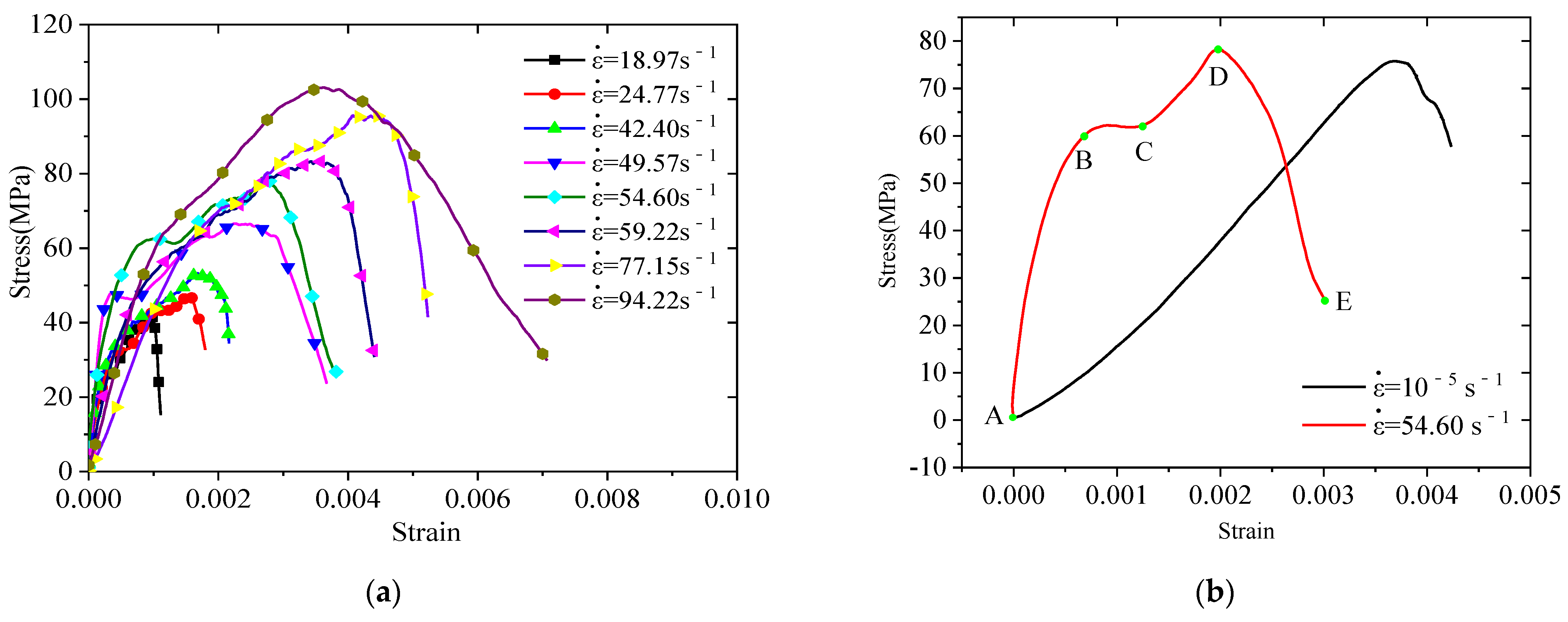
The basic mechanical parameters are RO, FC, G and T, which can be measured using uniaxial compression tests. The static stress–strain curves of sandstone specimens are shown in Figure 5b. According to the basic theory of rock mechanics, the mechanical parameters can be obtained as shown in Table 2.
The limit surface parameters include A, B, N and SFMAX. The influence of the damage and strain rate is not considered in the determination of the limit surface parameters; thus,
σ * = A + B · p * N
The limit surface of the HJC model and the envelope of the Mohr–Coulomb (M-C) criterion start from the same point and have an intersection, as shown in Figure 13. In the M-C criterion, the intercept C of the envelope is the cohesion, which is obtained via a series of triaxial compression tests. Therefore, the triaxial compression tests of sandstone under different confining pressures are carried out, as shown in Figure 14 and Table 3, and the established series of Mohr’s circles is shown in Figure 15. Here, σ 1 and σ 3 denote the confining pressure and axial pressure at failure, respectively. The common tangent of the series of Mohr’s circles was assessed, and the C value was 22.61 MPa.
The limit surface of the HJC model and the envelope of the M-C criterion pass through the same point (0, C):
C σ c = A
Thus, the value of A is 0.297. In the triaxial compression test, the failure strength increases with increasing confining pressure. After a series of triaxial tests under different confining pressures, a set of p * and σ * values can be obtained using Equations (22)–(25).
p = σ n + 2 σ r 3
Δ σ = σ n σ r
p * = p f c
σ * = Δ σ f c
where σ n   is the axial pressure corresponding to sandstone failure in the triaxial test; σ r is the confining pressure; and p * and σ * are the normalized hydrostatic pressure and normalized stress difference, respectively, as shown in Table 4. Figure 16 shows the relationship between p * and σ * by using Equation (26):
σ * = B · p * N
Figure 15 shows that the values of B and N are 1.947 and 0.537, respectively.
S F M A X is the ratio of the stress difference when the axial compressive strength of the specimen does not increase with increasing confining pressure from the triaxial test to the static compressive strength:
S F M A X = Δ σ max σ c
According to the triaxial compression test results, the axial pressure remains stable when the confining pressure is approximately 90 MPa. The limit surface parameters of sandstone are shown in Table 5.
The strain-rate-dependent parameters include C and EPSO. The parameter C is obtained by using a single impact test under different strain rates. In addition, the influence of the hydrostatic pressure on σ d * and ε ˙ should be eliminated in the calculation of the parameter C. The specific method is as follows: σ d * and the corresponding ε ˙ are taken when σ d * is approximately 1 / 3 σ d * ; then, the relationship between the obtained series of σ d * and ε ˙ is fit with a linear equation, the slope of which is the value of C. Here, the normalized dynamic compressive strength is introduced:
σ d * = σ σ c
where   σ d * is the normalized dynamic compressive strength. The corresponding points of σ d * and ε ˙ for sandstone are shown in Table 6, and the fitting relationship is shown in Figure 17. The strain rate coefficient C is 0.0127. The reference strain rate EPSO is a fixed value, i.e., 1.0.
P C = σ c 3
U C = P C K
U L = ρ g r a i n ρ 1
where P C and UC are the hydrostatic pressure and volume strain corresponding to the elastic limit, respectively, and UL is the volumetric strain at plastic deformation. PC, UC and UL are calculated to be 25.38, 0.0016, and 0.08, respectively. The value of PL is determined by μ l in Figure 11c, and K1, K2 and K3 are determined by the stress amplitude and corresponding equivalent volumetric strain under impact loading. Therefore, it is necessary to carry out impact tests to obtain the fitting relationship by using Equation (32):
p = k 1 μ ¯ + k 2 μ ¯ 2 + k 3 μ ¯ 3
The relationship between the stress amplitude and equivalent volumetric strain under impact loading is shown in Figure 18. The parameters related to the state equation are calculated as shown in Table 7.
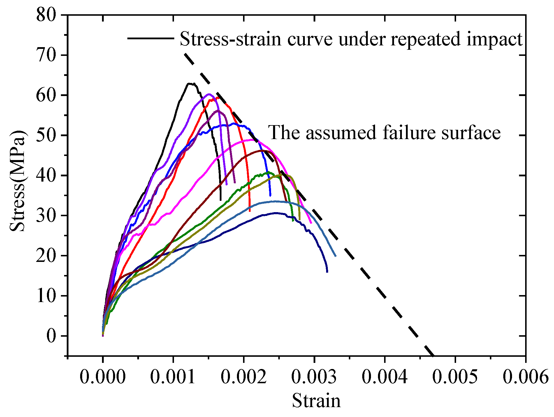
The damage parameters include D1, D2 and EFMIN. The damage in the HJC model is determined by the equivalent plastic strain and volumetric strain. When determining the parameter values of D1 and D2, it is assumed that the material is only damaged under repeated impacts, and that the corresponding damage value is 1, so the following equation is obtained:
ε p f + μ p f = D 1 ( p * + T * ) D 2
where ε p f + μ p f is the fracture plastic strain under repeated impacts. EFMIN is the failure strain under repeated impacts. The specific method is to draw a common tangent of the peak strength of the constitutive curve cluster obtained under repeated impacts, and the strain value corresponding to the intersection of the common tangent and the abscissa axis is the failure strain under repeated impacts, as shown in Figure 19. The failure strain of sandstone is 0.00465. The relationship between the strain and damage is determined by Equation (32). Since the repeated impact stress amplitude does not exceed the elastic limit of the sandstone, only recoverable elastic strain occurs in the sandstone at this time, and no plastic strain occurs. Therefore, the left part of Equation (32) is equal to the value of the failure strain. Additionally, it is assumed that the value of D2 is 1.0.32 The value of p* is 0.82, which is determined by the stress wave amplitude, and T* is 0.1002. The calculated value of D1 is 0.005.
In summary, a total of 19 parameters of the HJC model for sandstone were measured, which are shown in Table 8.

4.2. Application of the Parameter Determination Method in LS-DYNA

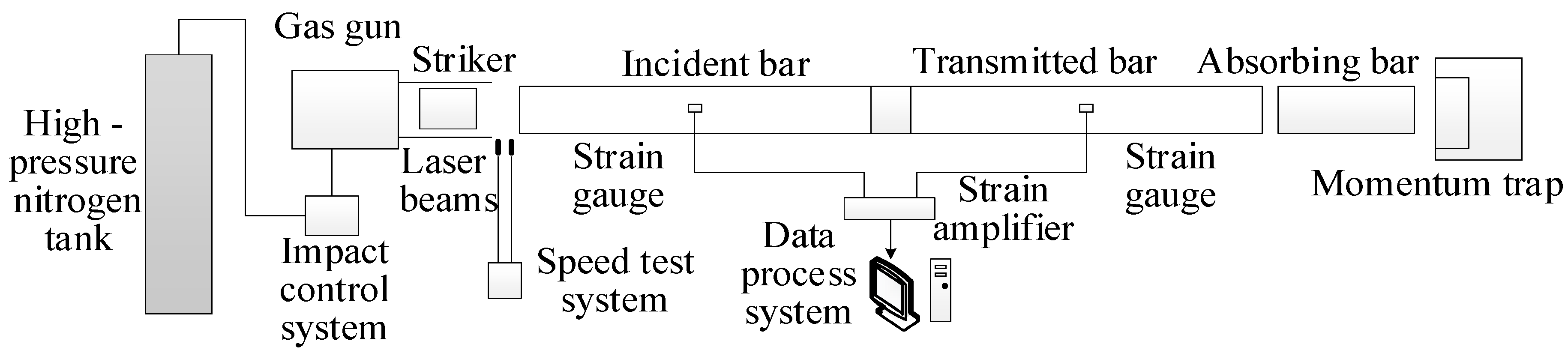
The model of the SHPB system with a diameter of 50 mm was established in LS-DYNA, as shown in Figure 20. The lengths of the impact bar, incident bar and transmitted bar are 400 mm, 2000 mm and 2000 mm, respectively. The diameter of the specimen is 50 mm, and the length is 40 mm. The material of the bar is defined as an elastic material, and the properties of the aluminum–magnesium alloy are a density of 2800 kg/m3, elastic modulus of 77 GPa and Poisson’s ratio of 0.27. The dynamic stress–strain curves of the sandstone under different impact velocities are extracted to calculate the elastic limit, peak strength, maximum strain and other mechanical indicators.
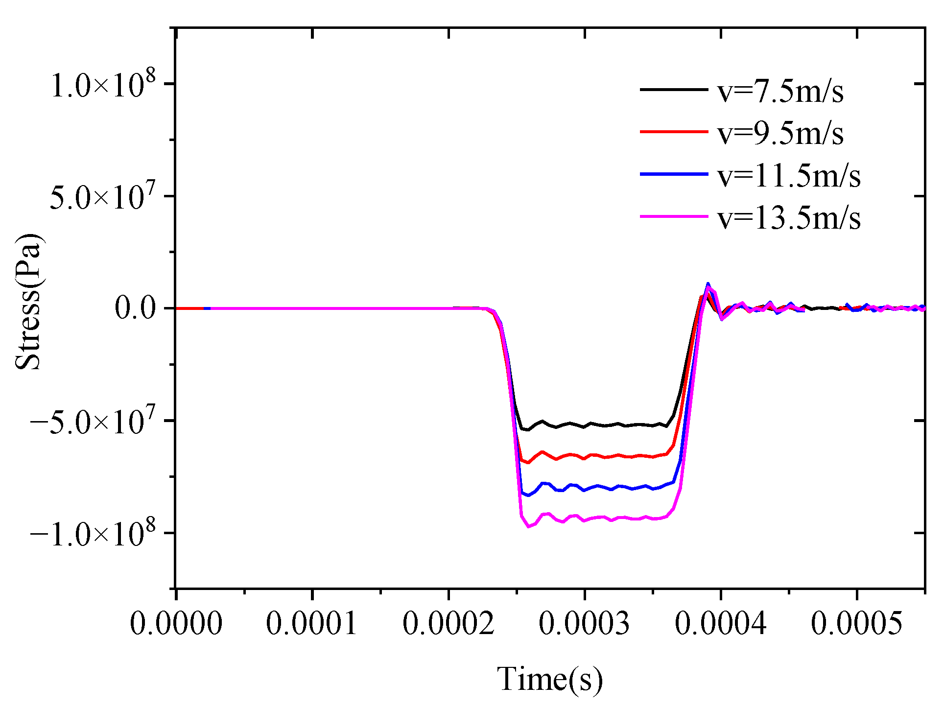
The impact velocities are taken as 7.5 m/s, 9.5 m/s, 11.5 m/s and 13.5 m/s, and the incident wave at each impact velocity is shown in Figure 21. The stress waves generated by the collision of elastic bars conform to the one-dimensional wave theory, and their amplitudes conform to the calculation results of σ = ρ Cv / 2 ; the durations are all 158.4 μs, consistent with the theoretical calculations.
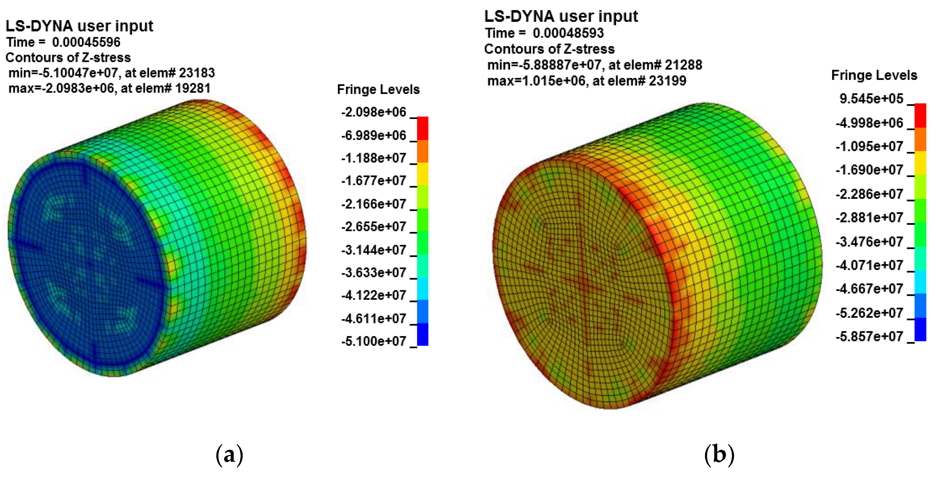
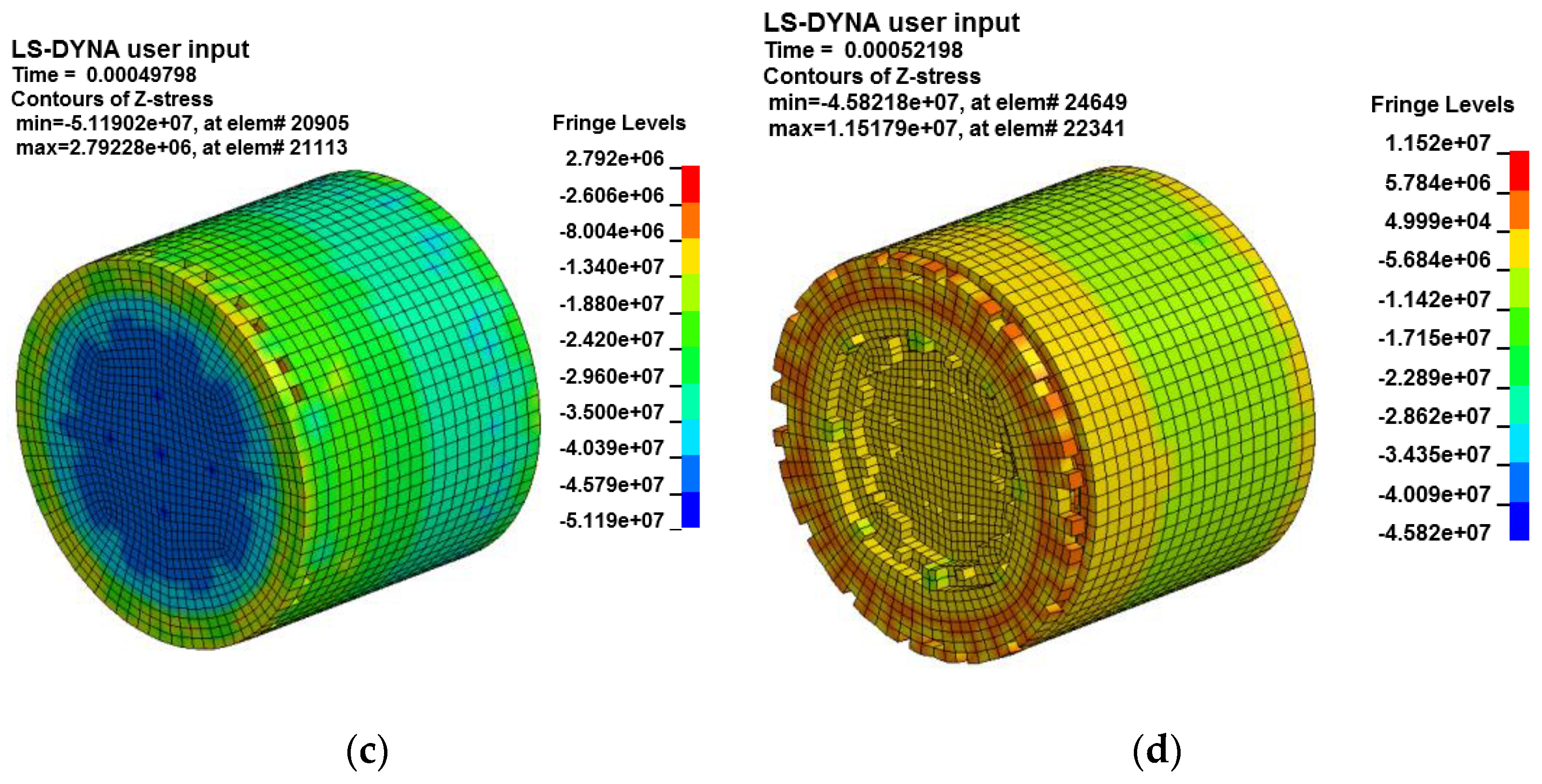
The stress and failure state of the specimen after the stress wave loading are intercepted, as shown in Figure 22. Figure 22a shows that the stress wave acts on the contact surface of the specimen and the input bar relatively uniformly at this time, and the maximum compressive stress is consistent with the amplitude of the incident wave; with the passage of time, the stress wave gradually moves towards the specimen. Internal propagation and action of the force occur, and stress reflection occurs on the end face of the specimen, with the stress cloud diagram shown in Figure 22b. Then, the internal compressive stress of the specimen gradually increases, individual elements meet the failure criteria and the element is deleted, indicating that the specimen begins to crack at the macroscopic scale. Finally, more elements are damaged and deleted, which shows the fracture of the specimen at the macroscopic level.
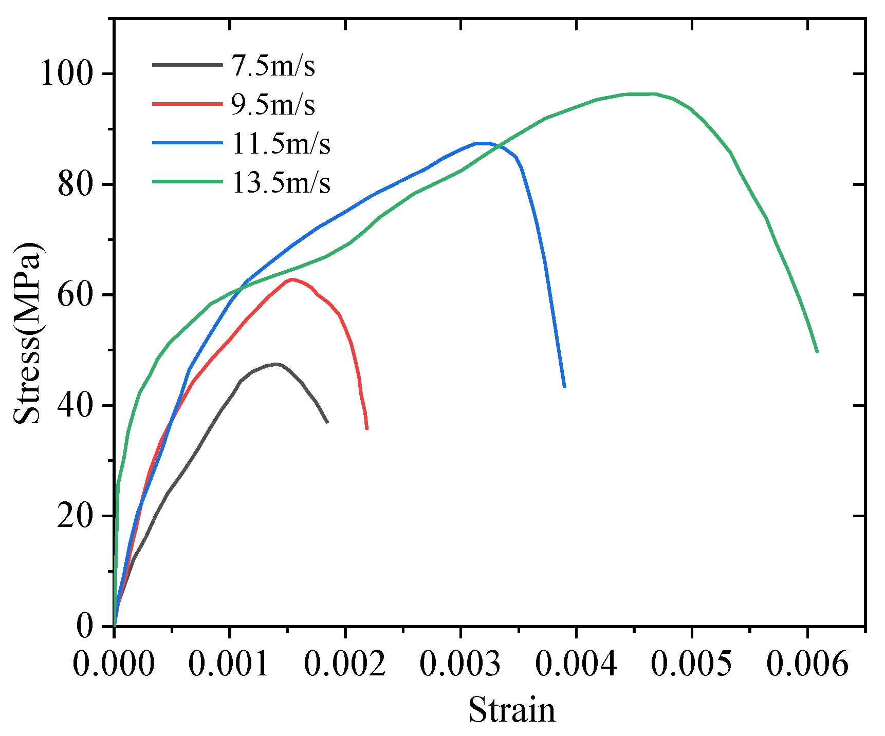
In LS-DYNA, the stress–time history curve and strain–time history curve of the object element can be directly extracted from the calculation results, and the stress–strain curve can be obtained after corresponding the two data points. A summary of the stress–strain curves is shown in Figure 23, which shows that with increasing impact velocity, the dynamic peak strength also increases, which conforms to the characteristic that the strength increases with the strain rate; at the same time, with increasing impact velocity, the dynamic elastic modulus of the curve also increases, which is also in line with the relevant situation for the previous SHPB trial. The dynamic mechanical properties of sandstone at each impact speed and a comparison with the test conditions are shown in Table 9.
Table 9 shows that the simulated strain rate, dynamic compressive strength and maximum strain of the sandstone specimen are highly similar to the experimental results under the same impact velocity, and the error does not exceed 10%. The method used for determining the parameters of the HJC model for rock materials provided in this paper is effective.

5. Conclusions

Single and repeated impact tests of sandstone specimens were carried out using a large SHPB setup. The dynamic stress equilibrium guaranteed the effectiveness of the test. Based on the analysis of the test results, the failure patterns and damage evolution law of the sandstone specimens were analyzed. Moreover, a set of methods for systematically determining the parameters of the HJC model for sandstone specimens was proposed. The main conclusions of this paper are as follows.
The typical dynamic constitutive curve of sandstone specimens is divided into four stages, namely the linear elastic stage, the new fracture formation stage, the plastic strengthening stage and the unloading stage. The failure mode of sandstone is mostly splitting tensile failure, and the impact damage threshold of sandstone is 45 J. The sandstone specimen under repeated impacts showed only one fracture surface compared with that subjected to a single impact.
The sandstone damage under a single impact is exponentially related to the stress wave amplitude. A model to describe the relationship between the damage and stress wave amplitude is D = 0.0029 · exp ( 5.4127 · σ / 76.13 ) 0.0504 . Under repeated impacts, the cumulative damage presented the development form of ‘rapid rise–steady development–rapid rise’, which can be expressed by the inverse transformation of the Goeppitz function, i.e., D = 0.265 0.328 · ln ( ln 13.989 / n ) .
The amplitude of the reflected wave and the area enclosed by the reflected wave and the abscissa axis gradually increase with an increasing number of impacts, while the transmitted wave amplitude and the area enclosed by the transmitted wave and the abscissa axis gradually decrease. As the number of impacts increases, the dynamic compressive strength and elastic modulus gradually decrease, while the strain corresponding to the peak stress increases gradually. The dynamic compressive strength decreases convexly with an increasing number of impacts. The maximum strain is positively correlated with the number of impacts.
The parameters of the HJC model are divided into five categories, namely the basic mechanical parameters, limit surface parameters, pressure parameters, damage parameters and rate effect parameters. A set of methods to determine the HJC model parameters for sandstone was proposed, which includes a single impact test, repeated impact test, uniaxial compression test and triaxial compression test. Then, the parameters for sandstone specimens were determined and used to simulate SHPB tests. The numerical simulation results showed that the strain rate, dynamic compressive strength and maximum strain of the sandstone specimen were highly similar to the experimental results. The method for determining the parameters of the HJC model for rock materials provided in this paper is effective.

Author Contributions

Conceptualization, S.L. and S.H.; methodology, S.W.; software, S.W.; validation, S.L., S.H. and S.W.; formal analysis, S.L. and S.H.; investigation, S.H.; resources, S.L.; data curation, S.L.; writing—original draft preparation, S.H.; writing—review and editing, S.H.; funding acquisition, S.L. All authors have read and agreed to the published version of the manuscript.

Funding

This research has been supported by the National Key R&D Program (2017YFC0804607) and the Fundamental Research Funds for the Central Region (2017QL05).

Institutional Review Board Statement

Not applicable.

Informed Consent Statement

Not applicable.

Data Availability Statement

The data that support the findings of this study are available from the corresponding author upon reasonable request.

Conflicts of Interest

The authors declare no conflict of interest.

References

  1. Hajiabdolmajid, V.; Kaiser, P. Brittleness of rock and stability assessment in hard rock tunneling. Tunn. Undergr. Space Technol. 2003, 18, 35–48. [Google Scholar] [CrossRef]
  2. Dehkhoda, S.; Hood, M. The internal failure of rock samples subjected to pulsed water jet impacts. Int. J. Rock Mech. Min. Sci. 2014, 66, 91–96. [Google Scholar] [CrossRef]
  3. Wang, G.H.; Lu, W.B.; Yang, G.D.; Yan, P.; Chen, M.; Zhao, X.H.; Li, Q. A state-of-the-art review on blast resistance and protection of high dams to blast loads. Int. J. Impact Eng. 2020, 139, 103529. [Google Scholar] [CrossRef]
  4. Herrmann, H.; Bucksch, H. Construction Geotechnical Engineer; Springer: Berlin/Heidelberg, Germany, 2014. [Google Scholar]
  5. Atkinson, B.K. Subcritical crack growth in geological materials. J. Geophys. Res.-Atmos. 1984, 89, 4077–4114. [Google Scholar] [CrossRef]
  6. Daniel, I.M.; Rowlands, R.E. On wave and fracture propagation in Rock Media. Exp. Mech. 1975, 15, 449–457. [Google Scholar] [CrossRef]
  7. Zhang, Q.B.; Zhao, J. A review of dynamic experimental techniques and mechanical behaviour of rock materials. Rock Mech. Rock Eng. 2014, 47, 1411–1478. [Google Scholar] [CrossRef] [Green Version]
  8. Kolsky, H. An investigation of the mechanical properties of materials at very high rates of loading. Proc. Phys. Soc. B 1949, 62, 676–700. [Google Scholar] [CrossRef]
  9. Khosravani, M.R.; Weinberg, K. A review on split Hopkinson bar experiments on the dynamic characterisation of concrete. Constr. Build. Mater. 2018, 190, 1264–1283. [Google Scholar] [CrossRef]
  10. Xia, K.W.; Yao, W. Dynamic rock tests using split Hopkinson (Kolsky) bar system—A review. J. Rock Mech. Geotech. 2015, 7, 27–59. [Google Scholar] [CrossRef] [Green Version]
  11. Hauser, F.E. Techniques for measuring stress-strain relations at high strain rates. Exp. Mech. 1966, 6, 395–402. [Google Scholar] [CrossRef]
  12. Dutta, P.K.; Kim, K. High-strain-rate tensile behavior of sedimentary and igneous rocks at low temperatures. CRREL Report, 1 October 1993. [Google Scholar]
  13. Dai, F.; Huang, S.; Xia, K.W.; Tan, Z.Y. Some fundamental issues in dynamic compression and tension tests of rocks using split Hopkinson pressure bar. Rock Mech. Rock Eng. 2010, 43, 657–666. [Google Scholar] [CrossRef]
  14. Deng, G.Q.; Yang, X.M. Comparative experimental investigation on damage process of rock under static cyclic loading and repeated dynamic impact. Chin. J. Rock Mech. Eng. 2014, 3, 581–585. [Google Scholar]
  15. Zhang, C.; Cao, W.G.; Wang, J.Y. A study of the statistical damage constitutive model for the brittle-ductile transition of rock with consideration of damage threshold. Hydrogeol. Eng. Geol. 2013, 5, 45–50+57. [Google Scholar]
  16. Zhu, J.J.; Li, X.B.; Gong, F.Q.; Wang, S.M.; He, W. Experimental test and damage characteristics of sandstone under uniaxial impact compressive loads. J. Cent. South Univ. 2012, 43, 2701–2707. [Google Scholar]
  17. Wu, B.; Kanopoulos, P.; Luo, X.; Xia, K. An experimental method to quantify the impact fatigue behavior of rocks. Meas. Sci. Technol. 2014, 25, 075002. [Google Scholar] [CrossRef]
  18. Luo, X.; Jiang, N.; Wang, M.; Xu, Y. Response of Leptynite subjected to repeated impact loading. Rock Mech. Rock Eng. 2016, 49, 4137–4141. [Google Scholar] [CrossRef]
  19. Li, X.B.; Lok, T.S.; Zhao, J. Dynamic characteristics of granite subjected to intermediate loading rate. Rock Mech. Rock Eng. 2005, 38, 21–39. [Google Scholar] [CrossRef]
  20. Jin, J.F.; Li, X.B.; Qiu, C.; Tao, W.; Zhou, X.J. Evolution model for damage accumulation of rock under cyclic impact loadings and effect of static loads on damage evolution. Chin. J. Rock Mech. Eng. 2014, 33, 1662–1671. [Google Scholar]
  21. Jin, J.F. Study on Rock Mechanical Properties under Coupled Static-Cyclic Impact Loadings; Central South University: Changsha, China, 2012. [Google Scholar]
  22. Li, X.; Main, I.; Jupe, A. Induced seismicity at the UK “hot dry rock” test site for geothermal energy production. Geophys. J. Int. 2018, 214, 331–344. [Google Scholar] [CrossRef] [Green Version]
  23. Li, S.H.; Zhu, W.C.; Niu, L.L.; Yu, M.; Chen, C.F. Dynamic characteristics of green sandstone subjected to repetitive impact loading: Phenomena and mechanisms. Rock Mech. Rock Eng. 2018, 51, 1921–1936. [Google Scholar] [CrossRef]
  24. Holmquist, T.J.; Johnson, G.R. A computational constitutive model for glass subjected to large strain, high strain rates and high pressures. J. Appl. Mech. 2011, 78, 051003. [Google Scholar] [CrossRef]
  25. Riedel, W.; Kawai, N.; Kondo, K.I. Numerical assessment for impact strength measurements in concrete materials. Int. J. Impact Eng. 2009, 36, 283–293. [Google Scholar] [CrossRef] [Green Version]
  26. Johnson, G.R.; Holmquist, T.J. High Pressure Science and Technology; American Institute of Physics: New York, NY, USA, 1993. [Google Scholar]
  27. Li, C.W.; Wang, J.G.; Xie, B.J.; Sun, Y.F. Numerical simulation of SHPB tests for coal by using HJC model. J. Min. Saf. Eng. 2016, 33, 158–164. [Google Scholar]
  28. Fang, Q.; Kong, X.Z.; Wu, H.; Gong, Z.M. Determination of Holmquist-Johnson-Cook consitiutive model parameters of rock. Eng. Mech. 2014, 31, 197–204. [Google Scholar]
  29. Zhou, Y.X.; Xia, K.; Li, X.B.; Li, H.B.; Ma, G.W.; Zhao, J.; Zhou, Z.L.; Dai, F. Suggested methods for determining the dynamic strength parameters and mode-I fracture toughness of rock materials. Int. J. Rock Mech. Min. 2012, 49, 105–112. [Google Scholar] [CrossRef]
  30. Xing, H.Z.; Zhang, Q.B.; Ruan, D.; Dehkhoda, S.; Lu, G.X.; Zhao, J. Full-field measurement and fracture characterisations of rocks under dynamic loads using high-speed three-dimensional digital image correlation. Int. J. Impact Eng. 2018, 113, 61–72. [Google Scholar] [CrossRef]
  31. Mehta, P.K.; Monteiro, P.J.M. Concrete: Microstructure, Properties, and Materials; McGraw-Hill: New York, NY, USA, 2006. [Google Scholar]
  32. Chen, J.L.; Li, X.D.; Liu, K.X. Experimental research on parameters of constitutive model for a cement mortar. Acta Sci. Nat. Univ. Pekin. 2008, 44, 689–694. [Google Scholar]
Figure 1. Schematic diagram of the SHPB experimental system.
Applsci 12 08366 g001
Figure 2. Verification of the dynamic stress equilibrium for typical specimens. Note: In, Re and Tr represent incident, reflected and transmitted, respectively.
Applsci 12 08366 g002
Figure 3. Waveforms of typical SHPB tests at different impact velocities.
Applsci 12 08366 g003
Figure 4. Strain rate–time curve.
Applsci 12 08366 g004
Figure 5. The stress–strain curves of sandstone specimens. (a) Dynamic stress–strain curves of sandstone specimens under different impact velocities. (b) Comparison between the typical dynamic and static stress–strain curves of sandstone specimens.
Applsci 12 08366 g005
Figure 6. Relationship between damage and incident stress wave amplitude under a single impact.
Applsci 12 08366 g006
Figure 7. The failure pattern of sandstone under a single impact.
Applsci 12 08366 g007
Figure 8. Waveforms of repeated SHPB impact tests.
Applsci 12 08366 g008
Figure 9. Dynamic stress–strain curves of sandstone specimens under repeated impact tests.
Applsci 12 08366 g009
Figure 10. The fitting curve of cumulative sandstone damage under repeated impacts.
Applsci 12 08366 g010
Figure 11. The failure morphology of sandstone under repeated impacts.
Applsci 12 08366 g011
Figure 12. The HJC model.
Applsci 12 08366 g012
Figure 13. Relationship between the HJC limit surface and the M-C envelope.
Applsci 12 08366 g013
Figure 14. Relationship between the stress and strain of sandstone under triaxial compression tests.
Applsci 12 08366 g014
Figure 15. The envelope of the M-C criterion for sandstone.
Applsci 12 08366 g015
Figure 16. The relationship between p * and σ * .
Applsci 12 08366 g016
Figure 17. The relationship between σ d * and ε ˙ for sandstone.
Applsci 12 08366 g017
Figure 18. The fitting relationship between p * and μ ¯ .
Applsci 12 08366 g018
Figure 19. The failure strain under repeated impacts.
Applsci 12 08366 g019
Figure 20. The SHPB model.
Applsci 12 08366 g020
Figure 21. The incident stress wave under different impact velocities in LS-DYNA.
Applsci 12 08366 g021
Figure 22. The simulation results of the specimen failure process. (a) Stress wave acting on the specimen. (b) Propagation of the stress wave to the specimen. (c) Sporadic unit failure. (d) Overall failure of the specimen.
Applsci 12 08366 g022aApplsci 12 08366 g022b
Figure 23. The numerical calculation results using the HJC model with the calibrated parameters.
Applsci 12 08366 g023
Table 1. Classification of HJC model parameters.
ParameterImplicationCategoryParameterImplicationCategory
ROMass densityBasic mechanical parametersPCCrushing pressurePressure parameters
FCQuasi-static uniaxial compressive strengthUCCrushing volumetric strain
GShear modulusPLLocking pressure
TMaximum tensile hydrostatic pressureULLocking volumetric strain
ANormalized cohesive strengthLimit surface parametersK1Pressure constant
BNormalized pressure-hardeningK2Pressure constant
NPressure-hardening exponentK3Pressure constant
SFMAXNormalized maximum strengthD1Damage constantDamage parameters
CStrain rate coefficientStrain rate dependent parametersD2Damage constant
EPSOQuasi-static threshold strain rateEFMINAmount of plastic strain before fracture
Table 2. The basic mechanical parameters of sandstone.
RO (kg/m3)FC (MPa)G (GPa)T (MPa)µE (GPa)K (GPa)
261076.1310.497.630.2225.6015.24
Table 3. The axial compressive strength under different confining pressures.
Confining PressureAxial Pressure
2.596
5.0110
6.0116
7.5123
10.0127
12.5129
Table 4. The values of p, Δ σ , p * and σ * under different confining pressures.
p Δ σ p * σ *
33.893.870.441.23
40.1105.400.531.38
43.0110.860.561.46
46.0115.510.601.52
49.0117.260.651.54
Table 5. The limit surface parameters of sandstone.
ABNSFMAX
0.31.950.541.2
Table 6. Dynamic compressive strengths of sandstone under different strain rates.
Strain Rate ε ˙ (s−1) Dynamic Compressive Strength (MPa)Normalized Dynamic Compressive Strength σ d *
85.1478.711.0
90.4380.321.1
95.8787.821.2
87.9695.981.3
100.74102.381.3
102.7496.791.2
120.18116.81.5
130.06125.141.6
Table 7. The pressure parameters related to the material state.
PC (MPa)UCPL (MPa)ULK1 (MPa)K2 (MPa)K3 (MPa)
25.380.00165.220.0810.67−62.56157.8
Table 8. The parameters of the HJC model for sandstone.
ParameterValueParameterValue
RO (kg/m3)2610PC (MPa)25.38
FC (MPa)76.13UC0.0016
G (GPa)10.49PL (MPa)5.22
T (MPa)7.63UL0.08
A0.297K1 (MPa)10.67
B1.947K2 (MPa)−62.56
N0.537K3 (MPa)157.8
SFMAX1.2D10.005
C0.0127D21.0
EPSO (s−1)1.0EFMIN0.00465
Table 9. Comparison between the simulation and experiment for the dynamic mechanical characteristics of sandstone.
CategoryImpact Velocity (m/s)Strain Rate (s−1)Dynamic Compressive Strength (MPa)Maximum Strain
Simulation7.5055.5348.081820
9.5064.0663.182170
11.5081.3688.943920
13.5085.2597.146080
Experiment7.5052.3950.932000
9.5064.7163.322260
11.5078.2395.873900
13.5090.69102.746017
Publisher’s Note: MDPI stays neutral with regard to jurisdictional claims in published maps and institutional affiliations.

