
Power System Inertia Dispatch Modelling in Future German Power Systems: A System Cost Evaluation


1
Wind Energy Technology Institute (WETI), Flensburg University of Applied Sciences, 24943 Flensburg, Germany
2
Interdisziplinäres Institut Umwelt-, Sozial- und Humanwissenschaften, Abteilung Energie- und Umweltmanagement, Europa-Universität Flensburg (EUF), 24943 Flensburg, Germany
Appl. Sci. 2022, 12(16), 8364; https://doi.org/10.3390/app12168364
Submission received: 26 July 2022
/
Revised: 17 August 2022
/
Accepted: 18 August 2022
/
Published: 21 August 2022
(This article belongs to the Special Issue Renewable Energy Systems: Optimal Planning and Design)
Abstract
:Increasing the share of grid frequency converter-connected renewables reduces power system inertia, which is crucial for grid frequency stability. However, this development is insufficiently covered by energy system modelling and analysis as well as related scientific literature. Additionally, only synchronous inertia from fossil fuel-emitting power plants is represented, although renewable generators are a source of synthetic inertia, thus resulting in increased must-run capacities, CO2 emissions and system costs. The work at hands adds an analysis of the future German power system considering sufficient inertia to the literature. Therefore, results of an novel open-source energy system model are analysed. The model depicts minimum system inertia constraints as well as wind turbines and battery storage systems as a carbon-dioxide-free source for a synthetic inertial response. Results indicate that integrating system inertia constraints in energy system models has a high impact on indicators such as system costs. Especially when investments in additional storage units providing an inertial response are necessary. With respect to researched scenarios, system cost increases range from 1% up to 23%. The incremental costs for providing additional inertia varies between 0.002 EURO/kg·m2 and 0.61 EURO/kg·m2.
1. Introduction
Energy systems are decarbonised to limit the consequences of climate change by integrating a Renewable Energy Source (RES). To a large extent, such state-of-the-art RES such as wind turbines and photovoltaic systems are connected to the power system via grid frequency converters [1]. Due to the fluctuating nature of feed-in from wind turbines and photovoltaic systems, the demand for energy storage systems increases [2]. Most short- and medium-term energy storage units are connected to the power system via grid frequency converters as well [3]. The integration of large shares of frequency converter-connected generation sources and energy storage units imposes considerable challenges on grid operators, power producers and authorities [4]. Grid frequency stability due to decreasing power system inertia is a challenge of increasing interest [1,5].
Sufficient power system inertia is the basis for grid frequency controllability [1]. The speed with which the grid frequency changes, also known as the Rate of Change of Frequency (ROCOF), is minimised by system inertia. Further, system inertia supplies time to units providing ancillary services such as primary frequency control to adapt power output [1]. The grid frequency is the indicator for power balance in AC power systems and has to be maintained within limitations for the purpose of power system security, e.g., to prevent disconnection of generators, interconnectors or power consumers [6,7]. The replacement of fossil-fuel-fired power plants and their synchronously connected generators by frequency converter connected RES reduces overall power system inertia [1]. Inertia can either be provided by synchronously connected rotating masses [1], e.g., synchronously connected generator or storage units, or emulated by frequency converter connected generation sources [8] and storage units [3]. An emulated inertial response is commonly referred to as Synthetic Inertia (SI) [1]. Hence, in future power systems, generation units and storage units also have to be dispatched intentionally with the purpose of securing sufficient system inertia.
Grid operators already face times with low inertia systems. The Canadian transmission network operator Hydro-Québec required wind turbines to provide an inertial response with the same performance as a synchronously connected generator in the case of a power imbalance [9,10]. The Irish Transmission System Operator (TSO) defines a frequency-sensitive mode for wind turbines [11] and curtails wind feed-in in times of low power system inertia [12]. Further, thresholds for non-synchronous penetration, the ROCOF and an operational limit for system inertia are defined [13]. The European Network of Transmission System Operators for Electricity (ENTSO-E) addresses the importance of inertia for grid frequency stability [4] as well as defining ROCOF withstand capabilities [14].
Although some power systems are already characterised by decreasing power system inertia, the development of system inertia in future power systems due to the integration of large shares of RES is a topic which has barely been focused on in energy system modelling. In general, energy system modelling is a key approach for energy system analysis [15] and aids in designing, planning and implementing future energy systems [16]. Four publications stand out in modelling inertia in future energy systems. Teng et al. analysed the 2030 Great Britain electricity network applying a unit commitment and economic dispatch model [17]. The ROCOF threshold is increased stepwise from 0.5 Hz/s up to 0.2 Hz/s to determine needed system inertia and assesses the impact on the system dispatch. In conclusion, a ROCOF threshold of 0.2 Hz/s will result in a 120% increase of operation costs as well as increased wind feed-in curtailment of 35%. Collins et al. implemented a 0.75 Hz/s rocof threshold into the PRIMES-REF 2030 European Union (EU) scenario analysing wind and PV curtailment, levels of interconnector congestion and power prices [18]. An energy system disptach model was created applying the modelling tool PLEXOS. Ireland’s RES curtailment increased by 11% and the average interconnector congestion during 24% of the modelled time periods. Minimum inertia requirements on the other side are neglectable for Continental Europe, since sufficient inertia is shared amongst member countries. Johnson et al.’s objective is to close the gap of knowledge of insufficient inertia in unit commitment and dispatch models [19]. Therefore, a linear programming model of the ERCOT power system using PLEXOS software is created. When constraining inertia to meet minimum thresholds, fossil-fuel-fired generation plants are dispatched, resulting in increased system costs of $85 million. Mehigan et al. also implemented a rocof threshold into a mixed linear integer programming model of the European power system, analysing effects on curtailment of variable RES, carbon dioxide emissions and production costs [20]. A ROCOF threshold of 1 Hz/s results in increased system costs by 53.1% and CO emissions by 48.9%. In conclusion, the four publications showed that inertia constraints result in increased must-run-capacities, as well as higher system costs and carbon dioxide emissions. It has to be highlighted that none of the presented publications included sources for SI such as wind turbines of battery storage systems, although they acknowledged their beneficial support or synchronous storage units [19,20].
The work at hand adds an evaluation of system costs because of the provision of inertia in the German power system to the literature. The German power system is already characterised by high shares of frequency inverter connected generation sources and ambitious goals in terms of RES integration [21]. Although embedded in the Continental European power system in which power system inertia is shared transnationally, it is assumed that in future power systems, inertia has to be provided by each country in a principle of joint action, likewise to primary frequency control [22]. Thereby it is to some extent ensured that power provided by an inertial response is not restricted by transmission capacities between member states. To evaluate system costs in the German power system, a novel unit commitment and economic inertia dispatch model is designed, applying an open-source modelling tool. Minimum inertia constraints are defined and sources for synchronous and SI are provided. The model’s innovative approach is to consider inertia not only by synchronously connected generators but also by synchronously connected storage units and the provision of SI from wind turbines and battery storage systems. Hence, sources for inertia are dispatched alongside variable RES and dispatchable units to supply power demand. Different energy system pathways are assessed, including the impact of fast frequency response and CO emission prices. Scenarios are based on the 2020 Ten-Year Network Development Plan (TYNDP) [23] and a 100%-res scenario based on the e-Highway 2050 study [24].
2. Methodology
Introduced hereafter are the methods applied in this work to model inertia as an integral part of a dispatch model of future German power systems. This includes, in particular, inertia constraints and sources providing synchronous and non-synchronous inertia. Beforehand, the elementary basis of system inertia and its functionality are explained.
2.1. Fundamentals of Power System Inertia
In AC electrical networks, the generation and consumption of power have to be balanced at any given point in time [6]. The indicator for such an equilibrium is the grid frequency, , the representation of the rotational speed of all synchronously connected rotating masses [6]. The grid frequency deviates from its nominal value in the event of an imbalance of power generation and consumption, [6]. The ROCOF, , which represents the speed with which the grid frequency changes, is determined by the overall provided inertia from all, synchronously to the system-connected rotating masses, , and depicted in Equation (1) [1].
Kinetic energy stored in the rotational motion of the synchronously connected machine is described by Equation (2), where is the stored kinetic energy of the unit g.
Commonly, the provided inertia of a single rotating mass connected synchronously to the power system is expressed via the inertia constant, H [6]. The inertia constant is the proportional ratio of the machines’ stored kinetic energy, , with respect to the units of 3. apparent power, [1,6].
The inertia constant describes the theoretical time a synchronously connected rotating mass, e.g., synchronously connected generator, is able to supply nominal power only by the generators’ stored kinetic energy [6]. In the same manner, the robustness of electrical systems in case of deviations between power generation and consumption can be expressed with the power system inertia constant, [1].
Generation and energy storage units which are connected to the power system via grid frequency converters are electronically decoupled from the power system. Hence, even if a rotating mass exists as in the case of wind turbines, their rotational speed is isolated from the electrical grid and stored kinetic energy is hidden [1]. However, such units are capable of emulating the inertial response of a synchronously connected rotating machine in the event of a power imbalance known as Synthetic Inertia (SI) [1,3]. The provided inertial power, is described by Equation (4) and determined by the emulated moment of inertia, , as well as the grid frequency and the ROCOF.
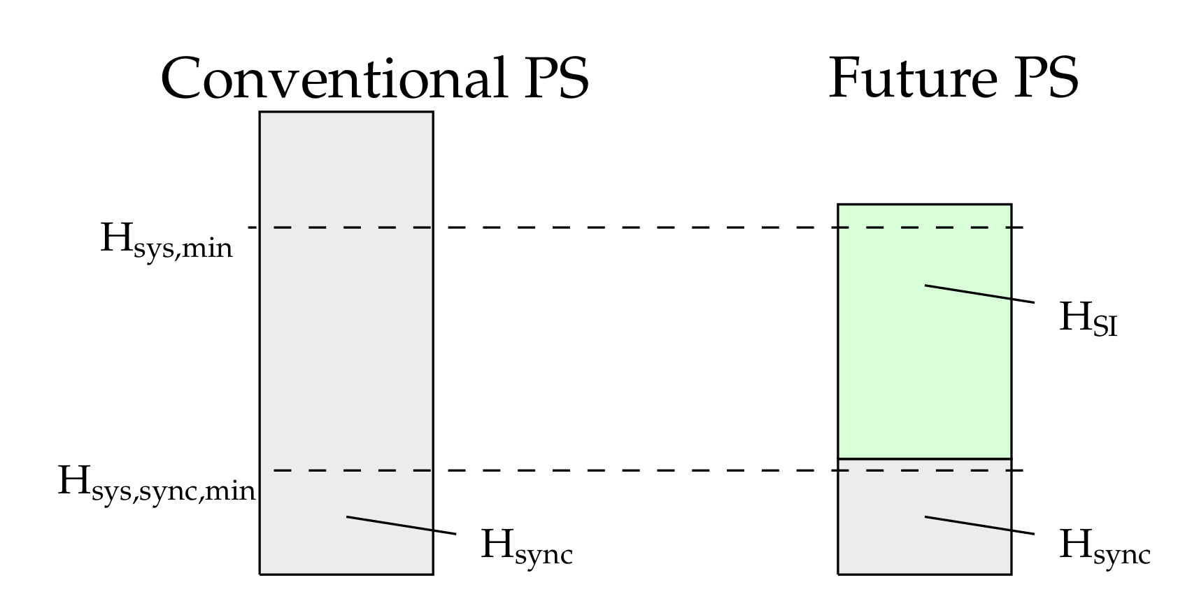
Inertia provided by synchronously connected rotating masses cannot directly be subsituted by SI [5]. The emulated inertial response is delayed due to the measurement of the grid frequency and precise detection of events which demand an inertial response [25]. Thus, to sustain controllability of the grid frequency in power systems with a high share of non-synchronous penetration, sufficient synchronous and non-synchronous inertia has to be provided. For synchronous inertia which responds instantaneously to limit the ROCOF, and non-synchronous inertia which is activated with a time delay after the power imbalance occurrence and synchronous inertia in combination, both provide time to units supplying grid frequency control servives and thus limiting the grid frequency nadir [1,25,26]. This is depicted in Equation (5) and further illustrated in Figure 1, in which is the provided synchronous inertia, is the provided non-synchronous inertia, the minimum required synchronous system inertia and the minimum required system inertia comprising a synchronous and a non-synchronous share. Thus, both requirements being met prevents ROCOF relays from triggering and the disconnection of loads or generation units due to the violation of grid frequency thresholds.
2.2. Unit Commitment and Dispatch Model Formulation
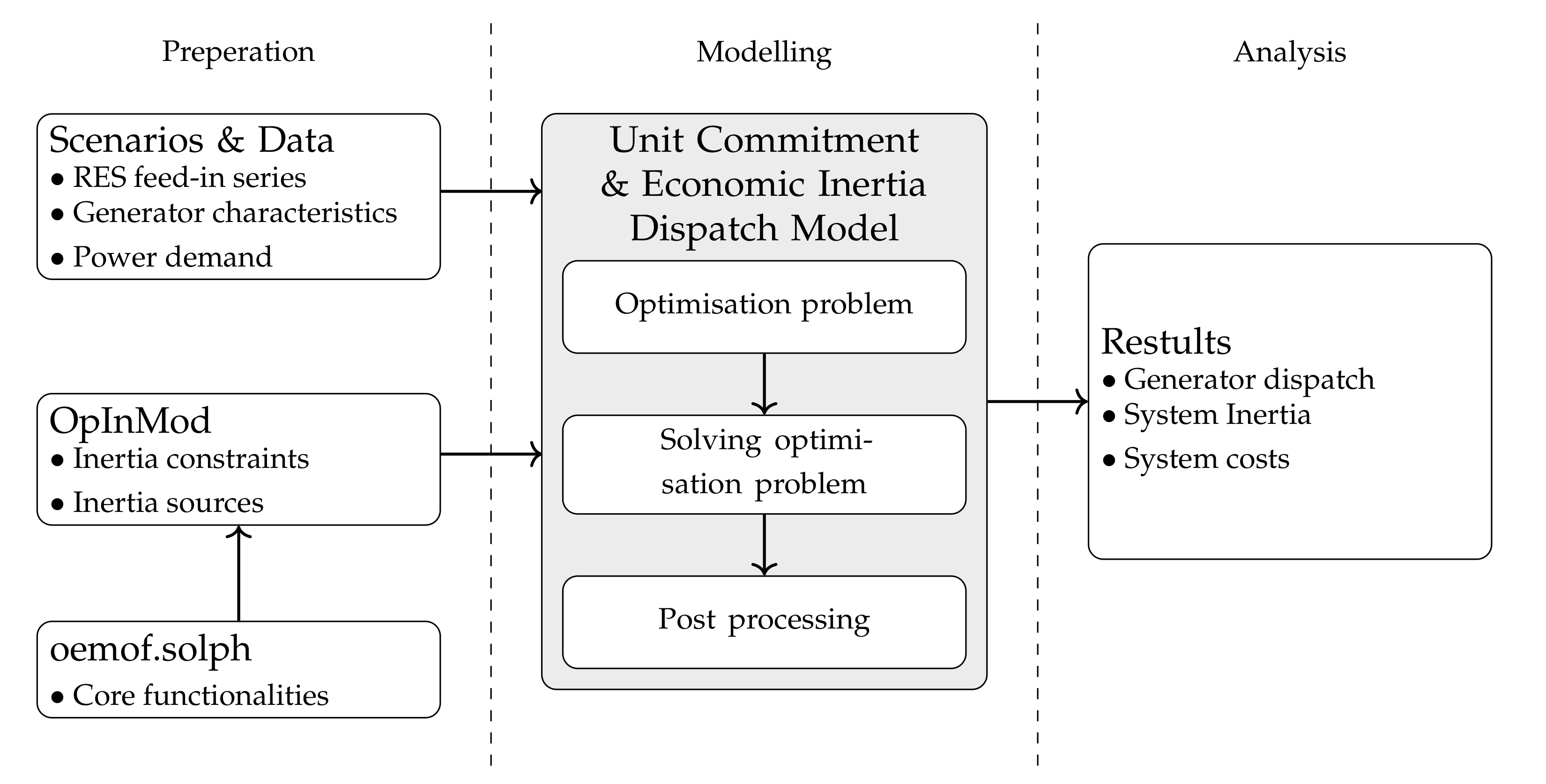
To evaluate system costs in the future German power system due to the provision of synchronous and non-synchronous inertia, the open-source modelling tool Open Inertia Modelling (OpInMod) is used. OpInMod is an open-source modelling framework able create unit commitment and economic inertia dispatch models [27]. It is built upon the basic functionalities of the Open Energy Modelling Framework (oemof) package solph [28,29]. OpInMod is implemented in python and inherits oemof’s design philosophy and core functionalities. Hence, scientific principles such as reproducibility, transparency and easy accessibility are met [30,31,32,33]. Like oemof.solph, OpInMod creates Mixed Integer Linear Programming (MILP) optimisation problems [29] applying python’s pyomo package [34]. An external solver is used to solve the optimisation problem. A simple validation and verification of OpInMod is presented in [27]. Therin, a stepwise presentation of OpInMods’s capabilites is shown. The presentation builds upon oemof’s examples which are provided alongside the model via Github [35]. Further, oemof itself has been reviewed and discussed in [36,37]. OpInMod is published under MIT License and can be accessed via Github [38] and zenodo [39]. A simplistic summary of the modelling procedure is illustrated in Figure 2.
In order to create a model of the German power system and to assess costs due to the provision of synchronous inertia and SI, the scenarios have to be defined first. Since the modelling tool OpInMod does not provide data by source, information such as feed-in series from wind turbines or solar photovoltaic system have to be provided. The same applies, e.g., for power demand series or generator characteristics such as the inertia constant or the generators’ efficiency. The unit dispatch and economic inertia dispatch model is created using OpInMod’s functionalities. This includes oemof’s core functions to represent energy systems. The created optimisation function of the unit dispatch and economic inertia dispatch model is solved by an external solver. The solver is freely selectable and has to be installed separately. Solver output is processed and transferred into a tabular data format for further analysis.
The optimisation function of the unit commitment and economic inertia dispatch model depicted in Equation (6) minimise the total system costs. The first term of the equation represents the costs of the energy flows by the variable costs of the unit, , and the flow variable, , and is inherented from oemof.solph [29]. The second part of the optimisation function describes inertia-related costs. The generators’ moment of inertia is depicted by and the costs of the unit providing inertia by . A synchronously connected rotating machine provides its total inertia to the power system while it is connected with the grid. The binary variable expresses this logic. Investment costs of storage units providing inertia, , are defined as the annualised inertia costs including fixed operation and maintenance costs.
The following paragraphs present how inertia is modelled within OpInMod and how constraints are created. Four sources for synchronous and non-synchronous inertia are implemented in OpInMod and presented hereafter. Although inertia is provided by synchronously connected loads as well [40,41], it is not incorporated into OpInMod. Research on the topic of load inertia is shallow [40,41], but more importantly, more loads in future power systems will be connected to the grid via frequency converters; thus, the inertial contribution of loads is further reduced [40].
2.2.1. System Inertia Constraints Formulation
As introduced in Section 2.1, future electrical grid systems will comprise of a minimum synchronous inertia part and a non-synchronous inertia part. To account for both system requirements in the unit dispatch model, two constraints are created. First, the minimum synchronous inertia constraint as expressed in Inequation (7) in which represents the minimum system inherent inertia while the right part of the Inequation the overall moment of inertia of all synchronously connected generators.
Second, the overall minimum system inertia requirement is depicted by Inequation (8). The minimum system inertia requirement is depicted via the variable . The right side of Inequation (8) shows the overall accumulated inertia of all connected generators providing either an inherent inertial response () or an non-inherent inertial response , i.e., SI.
2.2.2. Inertia by Synchronously Connected Generators
The first source able to provide inertia in the unit commitment and economic inertia dispatch model of the future German power system are synchronously connected generators. As indicated by the name, synchronously connected generators provide synchronous inertia. The inertia representation of synchronously connected generators and its characteristics are expressed via two constraints in this model. Shown by Inequation (9) is the first constraint. The energy flow variable, , of the synchronously connected generator has to be greater than the product of the generators nominated power, , and its lowest possible stable operation point, , per unit. Whether the synchronously connected generator is connected or disconnected from the power system is expressed by the binary variable .
The second constraint determines the value of the binary connection variable, , and is expressed by Inequation (10). The right side of Inequation (10) is a proportional expression of the synchronously connected units’ flow, , and the units’ nominated power, . As soon as the generators’ flow is greater then zero, the unit is connected to the system and thus supplies it total moment of inertia, i.e., . Thus, is set to the numeric value of one. Otherwise, the binary variables value is set to zero.
2.2.3. Inertia by Synchronously Connected Storage Units
Another source for synchronous inertia is synchronously connected storage units, and in this case, more precisely, synchronous condensers. Synchronous condensers are a source of inertia already in application but also used to provide ancillary services such as reactive power [42,43]. Since reactive power support is not part of the model, synchronous condensers in this model are only used for synchronous inertia provision. Synchronous condensers in the energy system model are either connected to the power system, i.e., providing full inertia, or are not connected to the power system and hence do not provide a synchronous inertial response.
2.2.4. Inertia by Wind Turbines
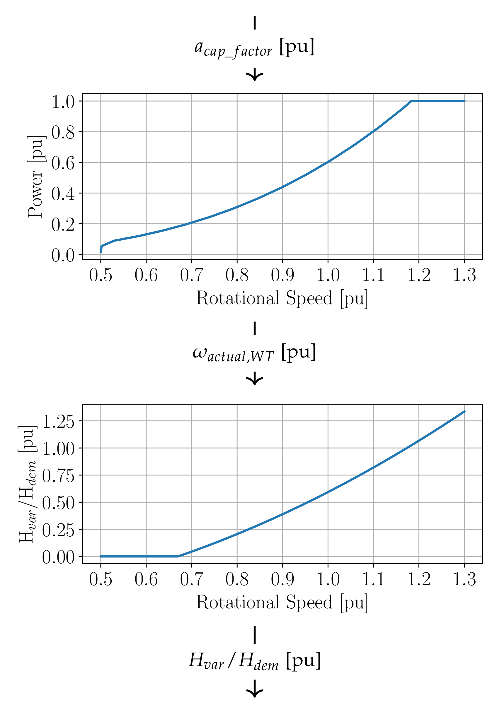
A source with a high potential for SI is wind turbines, which are thus integrated [1,8]. A common method to provide a synthetic inertial response with wind turbines is to adapt the electric power output with respect the power systems need, i.e., ROCOF and the grid frequency [1]. As a result, the wind turbines’ rotational speed changes, and stored kinetic energy is exchanged with the power system [44]. The wind turbine might then be operated at non-optimal rotational speed which could lead to undesired behaviour of the wind turbine and in worst case to the disconnection of the wind turbine due to over- or underspeed safety measures while providing a synthetic inertial response [8]. Thus, not only the SI support is lost, but the wind turbines’ regular non-inertia-related feed-in is lost as well [8]. To prevent such undesired consequences, the variable H controller is introduced by Gloe et al. [8]. The solution suggested by the authors is to scale the provided emulated moment of inertia with the actual operation point of the wind turbine. Therefore, the emulated inertial response is scaled with cut-in wind speed and the nominal speed of the wind turbine generator [8]. Hence, the risk of the wind turbine being disconnected from the grid is reduced while SI is provided. Therefore, the power systems’ demand for inertia is expressed by the inertia constant, [8]. It is defined by the respective TSO and based on the power systems’ specific requirements. The wind turbines’ variable inertia constant is normalised such that it is supplied at nominal speed [8].
A simplified approach to depict the potential provided SI with wind turbines based on the control concept of the variable H controller is implemented in OpInMod [27]. The method is illustrated in Figure 3. Since the simplified method to model wind inertia is based on the actual operation point of the wind turbine, normalised specifications of the open-source NREL 5 MW wind turbine generator are used [45,46]. The wind turbine’s operation point is used to determine corresponding normalised rotational speed. This is illustrated in the Figure 3 top subplot. Afterwards, the determined normalised rotational speed is used to specify the variable inertia constant, , with with regard to the demanded inertia constant, . This is visualised in the Figure 3 bottom subplot.
2.2.5. Inertia by Non-Synchronously Connected Energy Storage Units
The fourth source for inertia implemented is non-synchronously connected energy storage units. Different types of non-synchronously connected energy storage units can be applied to provide SI-like battery storage units [3,47]. Since most non-synchronously connected energy storage units do not have a physical rotating mass, the emulated moment of inertia, , is almost freely selectable, thus resulting in the SI power provision, , depicted in Equation (4). However, the maximum provided SI power provision is limited by the energy storage units’ rated power, , and the power output to balance power demand, , as depicted in Equation (11).
3. Scenario Design
The system costs evaluation in the work at hand is based on a unit commitment and economic inertia dispatch model of the German power system. Although the German power system is part of the Continental European power system and inertia is shared transnationally, it is assumed that in future systems, similar to primary load frequency control, inertia has to be provided by each member of the Regional Group of Continental Europe in a principle of joint action [22].
Each TSO has to contribute to primary load frequency control with respect to its contribution coefficient, which is the proportional expression of the generated electricity in the respective control block with respect to the overall generated electricity of all participants [22]. In a future power system when inertia is not a secondary product of power generation units and has to be provided intentionally to maintain controllability of the grid frequency, a similar regulation has to be established. Hence, a principle of joint action to share synchronous inertia and SI between the participants of the Continental European power system has to be introduced. It is calculated as depicted in Equation (13). Since such a regulation has to be implemented into national law by each member country, the analysis of this work is conducted for the future German power system, aggregating its current four control blocks, i.e., the four German TSOs.
As Germany is still embedded in the European power system and to account for cross-border flows, the neighbouring countries of Germany are modelled as well. However, only power generation is modelled, and provision of inertia for these countries is neglected. To reduce model complexity, smaller power systems are aggregated and grouped into single nodes: the Netherlands, Belgium and Luxemburg are grouped into one node; Switzerland and Austria are grouped into another node; and Poland and the Czech Republic are grouped into one node as well. France, Denmark, Sweden and Norway are each represented by a single node.
Three scenarios are designed, of which two are based on the 2020 TYNDP of the ENTSO-E [23], and one scenario is based on the e-Highway 2050 study [24]. A detailed description including all assumptions and limitations of the 2020 TYNDP scenarios is provided by the ENTSO-E [23,48] and of the scenarios of the e-Highway 2050 study [24]. Basic assumptions of the three scenarios are summarised in the following paragraphs:
- National Trends (NT): The NT scenario from the 2020 TYNDP sums up the individual commitments and climate policies of the EU member states fixed in the National Energy and Climate Plans CO emission reduction target lines, with the requirement to meet European 2030 energy strategy targets. The power sector in particular experiences a high increase in installed capacity of photovoltaic systems and wind turbine generators. Solutions for large-scale battery units are limited. Generators driven by natural gas or nuclear power replace fossil coal generation plants.
- Distributed Energy (DE): The DE scenario from the 2020 TYNDP is designed with a decentralised approach to meet the Paris Agreement Objective of an average global temperature increase of 1.5 °C or at least well below 2 °C by the end of the century. Especially small-scale photovoltaic system solutions such as rooftop photovoltaic systems of power consumers actively participating in the transformation process and regional use of biomass are applied as well as high generation from onshore wind capacities.
- RE100: As indicated by the name, the RE100 scenario from the e-Highway 2050 study relies on a carbon-free 100% res future. Hence, nuclear and/or fossil-fuel-fired power plants are excluded from the generation mix. Photovoltaic systems and wind turbines are the most prominent generation sources in the generation mix.
4. Data
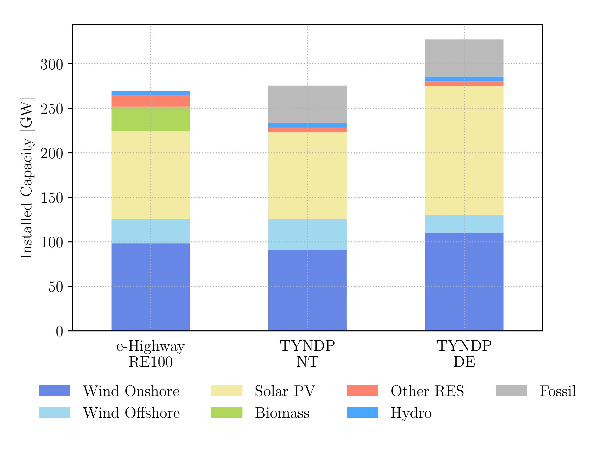
Data to model the DE and NT scenarios are extracted from the 2020 TYNDP of the ENTSO-E [23,49]. The data set provides installed capacities for conventional generation units, RES capacities, transmission line capacities and installed capacities for storage units, such as hydro pump storage units or battery storage systems [49]. The data sets to model the RE100 scenario are extracted from the e-Highway 2050 study [24,50]. Figure 4 provides an overview of the power generation mix per scenario and the respective installed capacities [49,50].
Table 1 provides an overview of commodity prices [49,51]. Specifications of conventional thermal power plants such as the units’ efficiency, the lowest possible point of stable operation and costs for Operation and Maintenance (O&M) are listed in Table 2 [51,52]. The results of a literature review summing up inertia constants for each generator type are also shown in Table 2 [20,53,54,55,56,57,58]. Costs for O&M in Table 2 vary with respect to the assumed CO emission prices as listed in Table 3. Also shown in Table 3 is the annual power demand for Germany for the respective scenario [49,50].
Investment options for storage units providing either a synchronous or an emulated inertial (SI) response are synchronous condensers or battery storage units, respectively. Synchronous condensers equipped with an additional flywheel system are a source of synchronous inertia already in application [42,43]. An overview of different battery storage systems providing SI is presented in [3]. Table 4 provides an overview of the parameters for the storage investment options. Inertia which has to be provided by storage untis translates into power and energy capacity. Applying Equation (4) translates the storage units’ inertia into power. The storage capacity is determined by incorporating the needed inertia from storage units into Equation (2). The methodology is also applied in [3]. The parameter WACC represents the weighted average capital costs.
Wind turbine and photovoltaic system feed-in time series in hourly resolution are provided by the Pan-European Climate Database. The data source provides a fixed power factor in a per unit quantity, per generation unit [61]. The power factor in per unit is applied to determine the provided SI with wind turbines as introduced in Section 2.2.4. Inflow of hydro units such as run-of-river plants is provided in a daily time resolution and for hydro reservoir and open pump storage units on a weekly basis [61]. The inflow profiles are converted into hourly inflow profiles.
As introduced above, the instantaneous ROCOF after the power imbalance is primarily determined by the system synchronous inertia, (see Equation (1)). The ROCOF has to be limited to avoid ROCOF relays from triggering [1]. Thus, grid components such as generators or interconnectors are not damaged by high ROCOF values [1]. According to the ENTSO-E, ROCOFs higher then 1 Hz/s are critical and might lead to chain reactions of negative events [26]. However, the ENTSO-E has also concluded that grid users in future power system shall be able to withstand a ROCOF of at least 2 Hz/s [26]. Therefore, the minimum system’s synchronous inertia, , to build the constraint depicted in Inequation (7) is determined by rearranging Equation (1) for assuming once a maximum ROCOF of 1 Hz/s and once considering a maximum ROCOF of 2 Hz/s. The power imbalance, , needed to determine is assumed to be the loss of the largest transmission line in the respective scenario. Currently, the power imbalance is the ENTSO-E reference incident, i.e., 3 GW [22]. However, the ENTSO-E concludes that the Continental European power system must be able to resist split scenarios, i.e., the loss of transmission lines or interconnectors [26]. The transmission line with the largest capacity, which in the case of its disconnection marks the worst-case scenario in terms of the power imbalance, is 6 GW for DE and NT scenario (a transmission line between France and Spain) and 10.4 GW for the RE100 scenario (a transmission line between Germany and Norway). Additionally, the nominal grid frequency, , of 50 Hz is assumed to calculate .
In future power systems, the combination of both synchronous inertia and SI is needed to limit the grid frequency nadir. To dimension the minimum needed system inertia and to build the constraint depicted in Inequation (8), a simplified grid frequency model which is also used in [3] is applied in this work as well. The model depicts the grid frequency development in the event of a power imbalance and calculates the grid frequency nadir considering the balancing effect of power system inertia and primary load frequency control with characteristics specified by the ENTSO-E [22]. A self regulation effect of loads of 1%/% is assumed [22]. The objective is to limit the grid frequency nadir to a lower bound of 49 Hz, since this is the lower threshold before load is shedded [22]. The needed system inertia is once determined assuming load frequency characteristics as currently specified [22], e.g., a deployment time of 30 s, and once considering the application of a fast frequency control service with a deployment time of 2 s as applied by the Irish grid operator [11].
Thereof, three parameter combinations of the ROCOF threshold and deployment time of primary load frequency control to limit the grid frequency nadir are combined to determine the required system synchronous inertia as well as the overall system inertia:
- (1)
- A minimum ROCOF of 1 Hz/s and a deployment time of 30 s representing the current system specifications. This parameter combination is hereafter referred to as 1 Hz/s, 30 s;
- (2)
- A minimum ROCOF of 1 Hz/s and a deployment time of 2 s. The parameter combination is hereafter referred to as 1 Hz/s, 2 s;
- (3)
- A minimum ROCOF of 2 Hz/s and a deployment time of 2 s, which is hereafter referred as 2 Hz/s, 2 s.
It is introduced in Section 3 that in the future Continental European power system, participants have to provide inertia in a principle of joint action likewise to current standards of primary frequency control [22]. Table 5 depicts the total energy generation in Germany and Continental Europe per scenario [49,50], as well as the resulting inertia contribution coefficient, , in percent as calculated when applying Equation (13). Table 6 provides an overview of the required system synchronous inertia and system inertia for Germany per scenario and parameter combination.
5. Results
To analyse system costs in future German power systems due to the provision of inertia, the scenarios are compared to the base scenarios. The base scenarios are optmised for each scenario (NT, DE and RE100) without consideration of provided inertia and system inertia constraints. Thus, the influence of of the inertia constraints on the dispatch and resulting system costs as well as carbon dioxide emissions can be isolated. As introduced in Section 3, two parameters which determine the required minimum system synchronous inertia as well as the minimum system inertia are varied. An overview of the parameter combinations and required system inertia parameters is provided via Table 6. Each possible scenario and parameter combination is optimised.
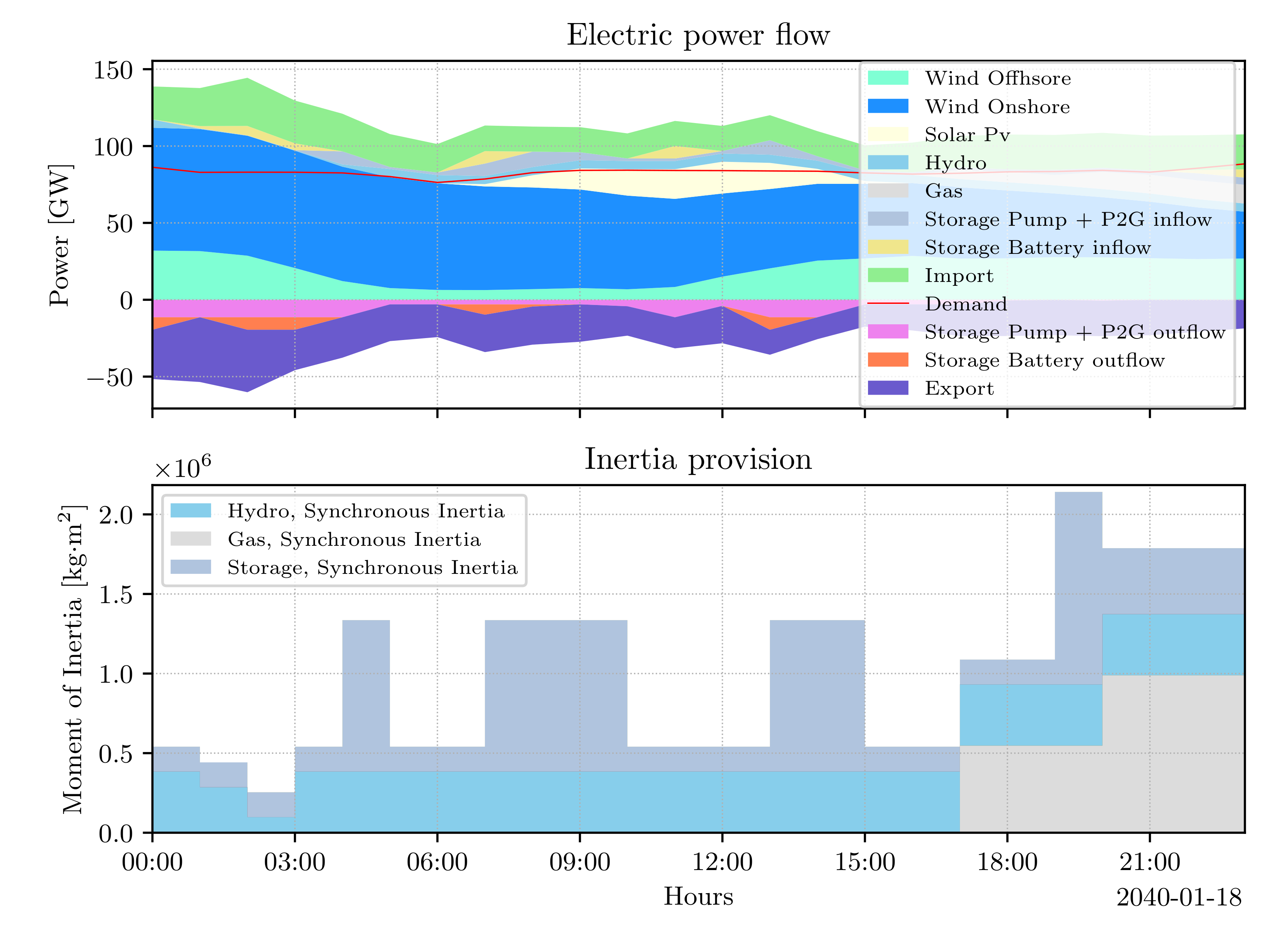
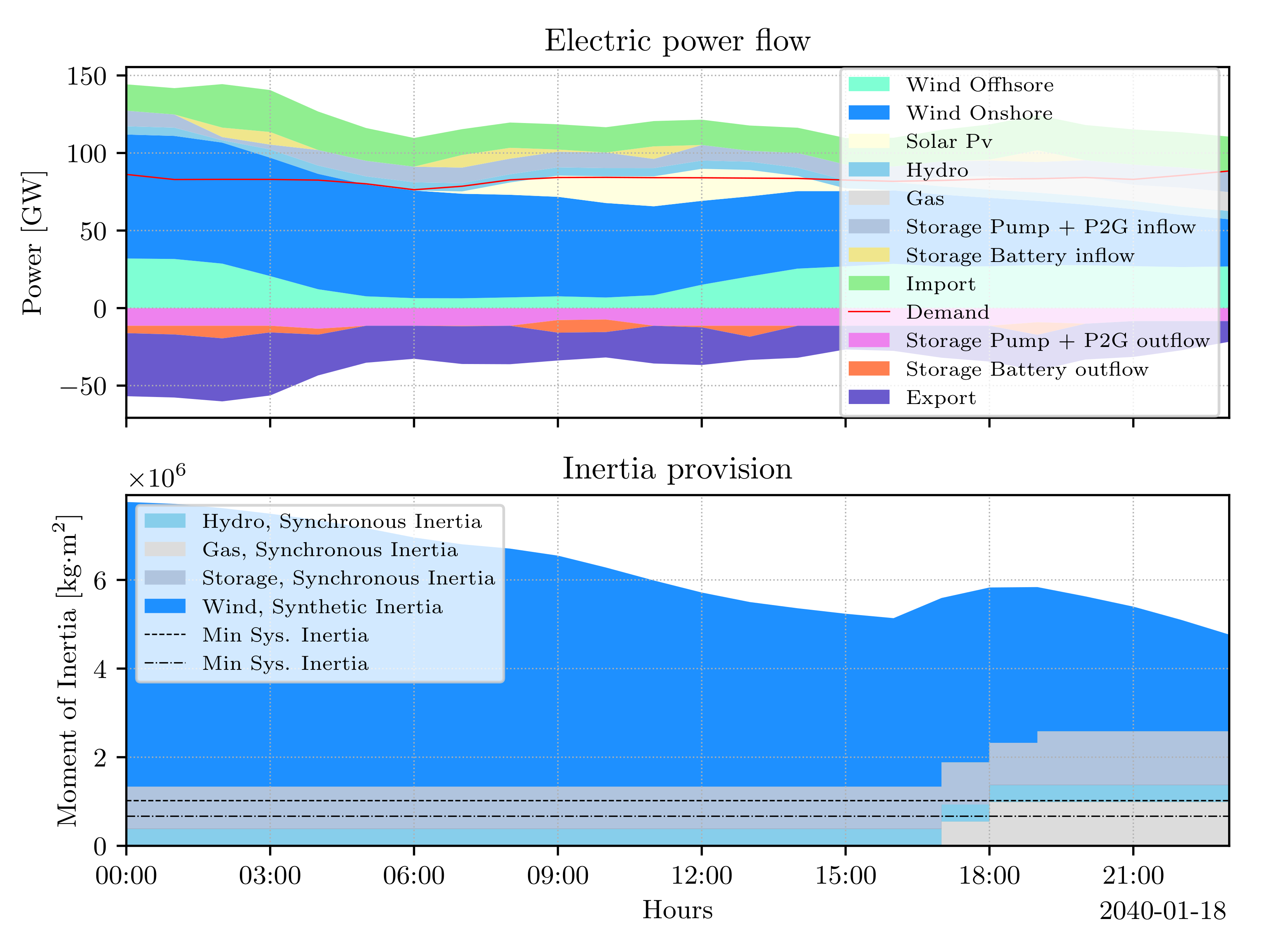
Figure 5 depicts a 24 h time series of the results of the NT base scenario without the consideration of inertia in the optimisation problem. To depict the influence of inertia constraints in the optimisation results, Figure 6 illustrates the exact same scenario and point in time as shown in the previous figure. However, Figure 6 shows results of the 1 Hz, 2 s parameter combination. The time series is selected randomly to illustrate the model’s functionality, hence the impact of the introduced inertia constraints on the flow and inertia output of dispatchable units. Thus, the presented results within the two figures are a qualitative validation of the model functionality and outcome. The top subplots of Figure 5 and Figure 6 each illustrate the electric power flow in GW. In positive direction of the y-axis, feed-in to the power system is depicted, i.e., generated power by RES or fossil-fuel-driven generation units and power output from storage units and imports from transmission cross-border units. In negative direction of the x-axis, cross-border outputs and energy inflow of energy storage units are shown. The bottom subplot shows the supplied moment of inertia in kg·m. In the previouly published literature, the supplied inertia is expressed via the system-wide stored kinetic energy or the system inertia constant of all connected synchronously generators [19,20,54]. As the wind turbine inertia provision concept introduced by Gloe et al. [8] is applied, the stored kinetic energy in the wind turbine’s rotor or wind turbine’s inertia constant is not an appropriate expression of the actual emulated inertia introduced by Gloe et al. [8]. Further, the moment of inertia in future systems should be introduced as a tradeable commodity [3].
The top subplot in Figure 5 shows the electric power flow results. Until 15:00 of the day, power demand could potentially satisfied by feed-in from onshore and offshore wind turbines as well as photovoltaic system feed-in. However, electric energy is still imported and at the same time exported. Hence, during this time, the German power system is a transit country for electrical energy. Electrical energy is also to a large extent stored in energy storage units such as batteries and pump storage units. By the end of the day, natural-gas-driven generators are dispatched to complement decreasing feed-in from onshore and offshore wind turbines and meet the power demand. During the first three hours of the day, hydro power plants and pump storage units are dispatched with minimum power output. Thereafter, with decreasing wind power feed-in, their output increases, thus resulting in the provided inertia as depicted by the bottom subplot during the first three hours of the depicted day. Thereafter, more units of these categories get connected to the system, which results in more inertia provided. Until 17:00, pump storage and power to gas units get connected to the system for a single hour, explaining the inertia peaks. As soon as gas-fired power plants get connected to the electrical grid, supplied inertia increases significantly.
Figure 6 depicts the results of the NT scenario and the 1 Hz/s, 2 s parameter combination. Again, feed-in from onshore and offshore wind turbines plus photovoltaic system feed-in during the midday could potentially satisfy power demand. However, due to the minimum synchronous inertia constraint and minimum system inertia constraint, more hydro and pump storage units are connected to the electrical grid until 17:00 of the day to meet the inertia constraints. This is visible when comparing the bottom subplots of Figure 5 and Figure 6. The inertia constraints are satisfied by hydro and pump storage units. Although the provided SI from wind turbines is high, pump storage and hydro units are both connected to the system to provide synchronous inertia, since the single connection of either of the units themselves would not be high enough to meet the system synchronous inertia constraint. Thus, both inertia constraints are met by the units providing an inherent inertial response, and SI by wind turbine generators would not be needed. However, due to the fact that inertia provision by wind turbines is not associated with costs and due to the model’s logic of the binary variable, , wind turbines provide full SI. By the end of the day, when natural-gas-driven generation units are connected to the electrical system to compensate decreasing feed-in from RES, synchronous inertia provided by such units increases.
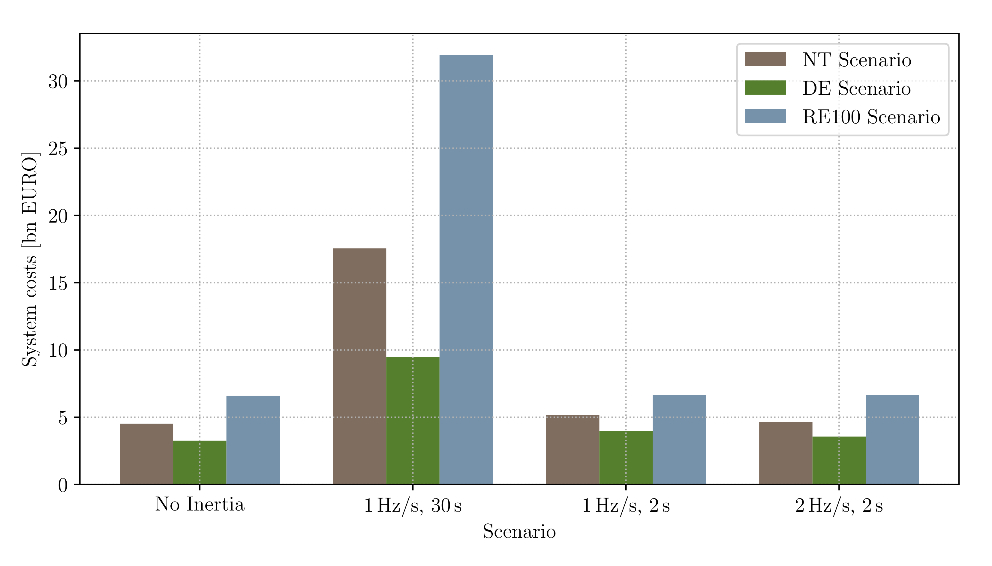
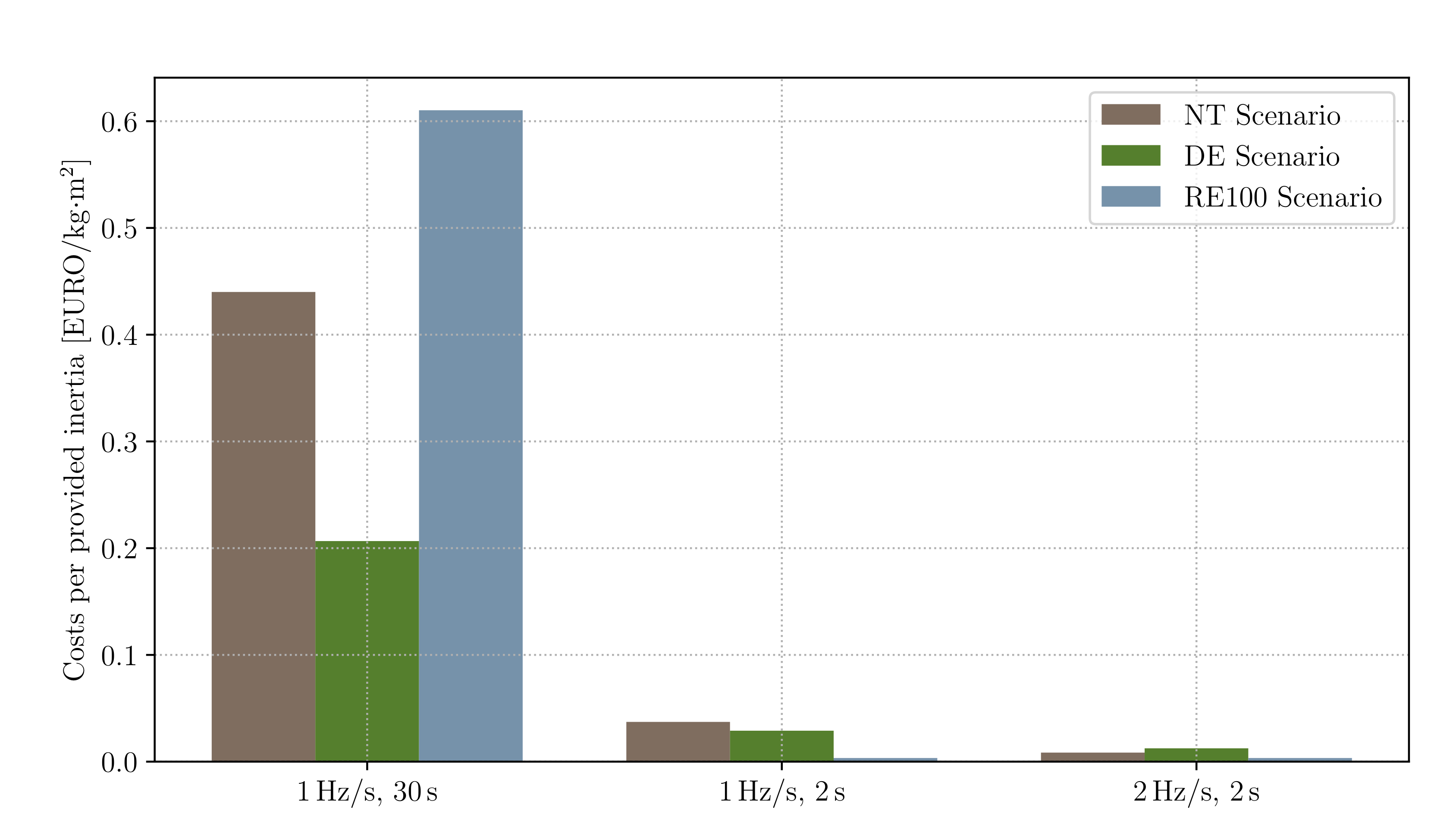
Table 7 provides an overview of the optimisation results for each scenario and parameter combination. Shown are results of overall CO emission, the number of synchronous condensers, the overall system costs and the costs for the provided inertia. The results of costs for the provided annual inertia are calculated by taking additional system costs due to the provision of inertia with respect to the additionally provided inertia to meet the inertia constraints and maintain grid frequency controllability. With respect to the base scenarios, carbon dioxide emissions for the 1 Hz/s, 30 s parameter combination of the NT as well as of the DE increase. In the NT scenario and parameter combination 1 Hz/s, 30 s, additional synchronous condensers provide a moment of inertia of overall 12 × 10 kg·m for the modelled time period. Battery storage units to provide a synthetic inertial response are not included by the model’s investment module. In the DE scenario and parameter combination 1 Hz/s, 30 s, synchronous condensers provided an overall additional moment of inertia of 6 × 10 kg·m. This investment optimisation result is reflected by higher system costs of bn 17.5 EURO for the NT scenario and bn 9.5 EURO for the DE scenario. The RE100 scenario and the parameter combination 1 Hz/s, 30 s, is also characterised by increased system costs of bn 31.9 EURO. Reducing the demand for overall inertia due to faster response of primary frequency control (from 30 s response time to 2 s time until full activation) results in decreasing system costs for the NT and DE scenario. However, CO emissions increase with respect to the base scenario. For these parameter combinations, it is overall less costly to dispatch fossil-fuel-fired power plants compared to investing in additional storage units providing synchronous inertia or SI. The last column of Table 7 depicts additional cost per provided additional inertia. Obviously, with decreasing demand for inertia, the cost per provided inertia decrease significantly. For the parameter combination 1 Hz/s, 30 s, to 1 Hz/s, 2 s, of the NT scenario, costs decrease from 0.44 EURO/kg·m to 0.04 EURO/kg·m. For the parameter combination 1 Hz/s, 30 s, to 1 Hz/s, 2 s, of the DE scenario, costs decrease from 0.21 EURO/kg·m to 0.03 EURO/kg·m and for the RE100 scenario from 0.61 EURO/kg·m to 0.003 EURO/kg·m.
Figure 7 depicts the overall system costs of each scenario and parameter combination in bn EURO. The overall system costs for all of the RE100 scenarios are higher, because investments in additional storage units providing inertia have to be conducted to meet the inertia constraints. The overall system costs of the DE scenarios are lowest for all parameter combinations. Figure 8 shows the additional system costs with respect to the additionally provided inertia due to the inertia constraints depicted as bar plots. Costs for inertia for the parameter combination of 1 Hz/s, 30 s, are highest in all scenarios due to the high investments. Decreasing the activation time of primary frequency control, resulting in less overall inertia needed, decreases the costs for additional inertia significantly.
6. Sensitivity Analysis
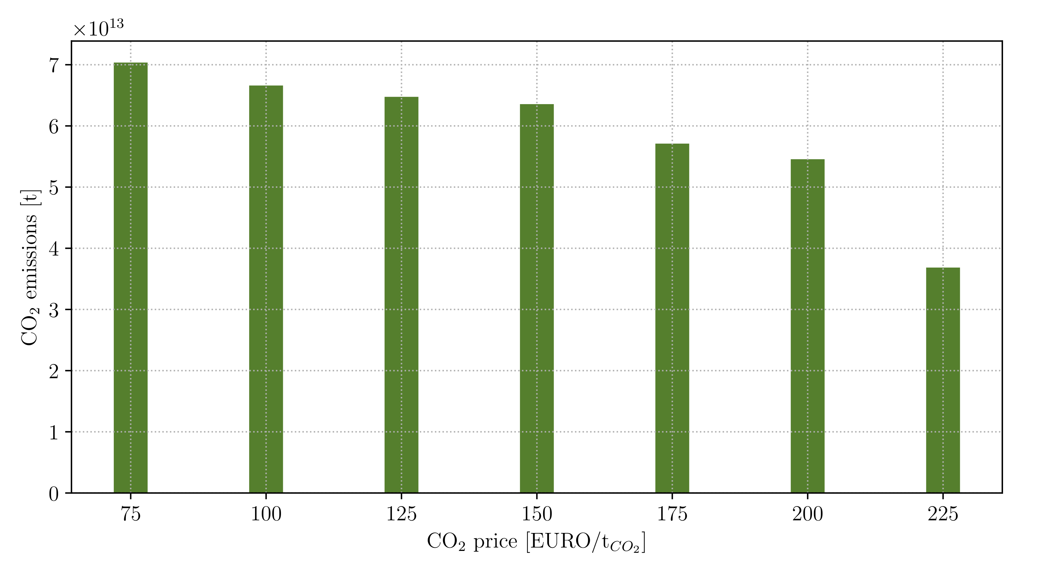
Results indicate that activation time for units providing primary frequency control services and thus the needed overall system inertia is one of the main drivers for increased overall system costs. However, carbon dioxide emissions increase at the same time. This is because it is more cost-efficient from a systems perspective to dispatch carbon-dioxide-emitting fossil fuel power plants than to invest in storage units providing synchronous inertia or SI. A market-driven solution would be to increase the costs for CO emissions, e.g., by decreasing the number of tradeable certificates. Figure 9 depicts the development of increasing prices for CO emissions for the NT scenario and 1 Hz/s, 2 s, parameter combination. For the analysis, price increments of 25 EURO/t are assumed. With increasing prices for CO emissions, as expected, emissions decrease. The highest change is visible for increased prices from 200 EURO/t to 225 EURO/t. Thereafter, carbon dioxide emissions do not decrease any further. In this case, fossil fuel generators are dispatched to meet power demand and not system inertia demand, hence, in times when power demand cannot be met by carbon-dioxide-emission-free generation or storage units.
As already introduced, the scenarios in this research are based on the TYNDP of the ENTSO-E and the e-Highway 2050 study. Since the designed scenarios are characterised by high installed capacities of weather-driven generation sources such as onshore wind, solar PV or run-of-river units, the respective weather input is of high influence to the results. The 2020 TYNDP applies three different climate years from the Pan-European Climate Database, namely the climate years from 1982, 1984 and 2007 [48,61]. The climate years are considered to be representative by the ENTSO-E [23]. To reduce complexity, the previous results are all modelled applying the 1984 climate year data sets. However, the impact of the climate years 1982 and 2007 on the overall system costs is analysed in this sensitivity section as well. Table 8 provides an overview of the climate years and their influence. For example, considering the factor Demand, it is highest for the climate year of 1984 compared to the climate years of 1982 or 2007. For Hydro Inflow, inflow is highest for the climate year 2007 compared with the climate years of 1982 and 1984.
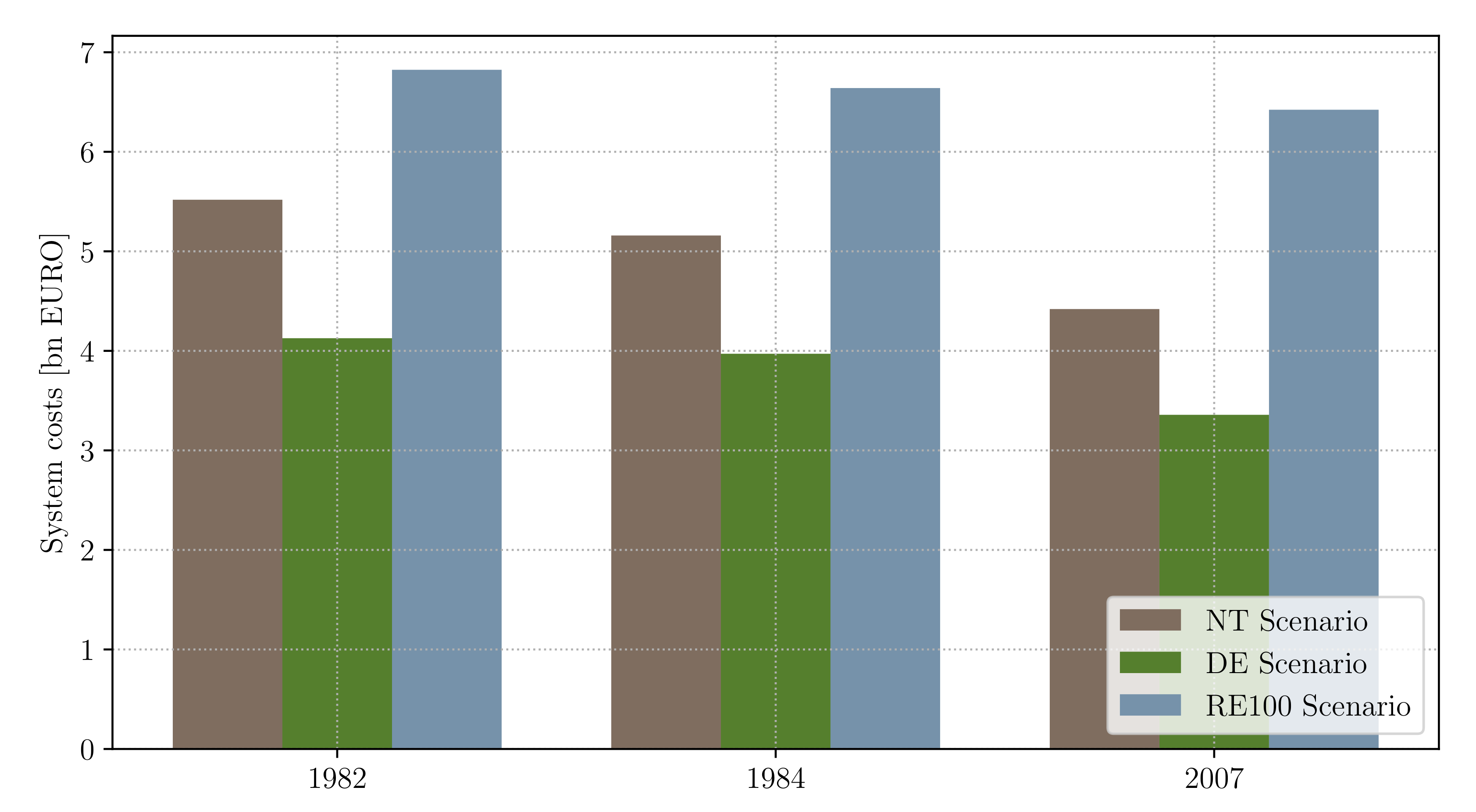
Each scenario and the parameter combination of 1 Hz/s, 2 s, has been analysed with respect to the three climate years. The results of the overall system costs are illustrated as a bar plot in Figure 10. For the climate year of 1982, system costs are highest since the potential for onshore and offshore wind is low. Hence, less SI is provided by such sources. Additionally, hydro inflow is in the middle region. Overall, this results in highest system costs compared to the other climate years and scenarios, since more inertia has to be provided by fossil-fuel-fired power plants and storage sources providing inertia. For the climate year of 1984, system costs are equally high. SI provision potential by onshore wind turbines in the middle region and inertia provision potential by hydro units is low. For the 2007 climate year, system costs are significantly lower, since the SI provision potential of onshore wind turbines and hydro units is highest.
7. Discussion
Comparing results of the work at hand with findings of the presented literature in the introduction (see Section 1), e.g., Collins et al. [18], Johnson et al. [19] or Mehigan et al. [20], shows some limitions of this resesearch in terms of comparability. All of the papers’ analysed scenarios take place in the year 2030. Hence, in the transition process of decarbonising energy systems, the scenarios analysed in the cited literature which include inertia constraints and modelling synchronous inertia are behind the scenarios analysed in this research. In this work, future German power system scenarios of the years 2040 and even 2050 are researched. The total RES penetration in the work of Johnson et al. is 30% [19]. The overall inverter-connected res penetration in the work of Collins et al. is 37% for Germany [18]. Non-synchronous penetration shares in the work at hand range from 77% up to 85%. This marks a significant increase compared to the discussed literature.
Still, system cost results presented in this work are comparable. Collins et al. conclude with a system cost increase of up to 37% [18]. Mehigan et al. conclude with system cost increases ranging from 43.1 to 58.1% based on the analysed scenario. System cost increases in this work range from 1% in the RE100 scenario to 14% in the nt scenario and 22% in the de scenario. It has to be noted that the lower results compared to Collins et al. and Mehigan et al. are of the 1 Hz/s, 2 s parameter combination and the resulting low demand for synchronous and overall system inertia. System cost increases for the 1 Hz/s, 30 s parameter combination, as indicated by Figure 7, are far higher due to the needed investment in storage units providing inertia. Such investments were not necessary in the discussed literature.
As already explained in the results section, in some scenarios it is more cost efficient to dispatch fossil-fuel-fired power plants capable of providing an inertial response in the event of a power imbalance than investing in newly added storage units. Increasing the price for carbon dioxide emissions (e.g., by reducing the number of tradeable CO certificates) is a market-based solution to decarbonise power systems while sufficient power system inertia is maintained. This approach increases system costs by 3.7 percent points at highest with respect to the 13% system cost increase in the nt scenario. Hence, pricing CO emissions is a reasonable approach to decarbonise power systems while maintaining sufficient power system inertia. Another potential solution to overcome this limitation is another constraint which restricts overall carbon dioxide emissions and thus results in investment and dispatch of additional carbon dioxide free storage units providing inertia.
8. Conclusions
Power system inertia is decreasing due to decarbonisation efforts and the integration of grid inverter connected power generation sources such as wind turbine generators and solar PV systems. Inertia is an essential part of grid frequency stability and therefore, a minimum synchronous system inertia as well as an overall system inertia, consisting of either a synchronous or an emulated share, has to be maintained. However, this development is not represented appropriately in energy system modelling. If considered at all, power system models only depicted inertia provision by synchronously connected generators of fossil-fuel-fired power plants. This results in increased carbon dioxide emission, must-run capacities and increased system costs and of course is contradictory to the general objective of modelling power systems with high shares of non-synchronously connected generation and storage systems.
The presented research closes the research gap of insufficient representation of power system inertia in energy system models. Therefore, an open-source unit commitment and economic inertia dispatch model of the future German power system is created and analysed. The power system dispatch model is created, applying the open-source modelling framework OpInMod. Dispatchable sources for synchronous inertia are synchronously connected generators and synchronously connected condensers. Dispatchables sources for SI are wind turbines as well as battery storage units. A 2040 power system model of the German power system is analysed based on data from the TYNDP as well as a 2050 100% res scenario of the e-Highway 2050 study of the ENTSO-E. Different parameter combinations of the maximum permitted ROCOF determining the required synchronous inertia as well as the maximum time until full activation of primary load frequency control determining the overall required power system inertia are analysed. Although the German power system is embedded in the Continental European power system in which power system inertia is shared transnationally, it is assumed that in future power systems, inertia has to be provided by each country in a principle of joint action likewise to primary frequency control.
Results show that retaining a full activation time of primary frequency control of 30 s as applied today, system costs increase significantly. Highest system costs occure in the 100% res scenarios of bn 31.924 EURO. System costs in the two 2040 scenarios are with bn 17.546 EURO and bn 9469 EURO lower in the NT and DE, respectively. High system costs in these scenarios are due to investments in additional synchronous condensers to meet inertia constraints. Decreasing primary load frequency control activation time to 2 s as for the case of fast frequency response, overall system costs can be reduced significantly to bn 6.6 EURO in the 100% res scenario and even down to bn 3.9 EURO in the DE. Allocating additional system costs to the additionally provided inertia results in values ranging from 0.002 EURO/kg·m to 0.61 EURO/kg·m.
The results indicate that in some cases, it is less costly to dispatch fossil-fuel-fired power plants to provide an inertial response than to invest in non-CO-emitting storage units. Hence, overall carbon dioxide emissions increase. Thus, a further analysis with increasing CO emission prices to support a market-based solution to decarbonise energy system has been conducted. CO emission prices of more than 225 EURO/t do not further decrease carbon dioxide emissions. In this case, fossil-fuel-fired power plants are dispatched independently from inertia constraints to meet power demand.
A further sensitivity analysis shows that in power systems based on a high share of supply-dependent generation sources such as wind turbines, times with less wind potential or hydro inflow result in increased system costs. At such times, alternative sources for SI or synchronous inertia have to be replaced with cost-intensive storage units or fossil-fuel-fired power plants to supply demand and provide sufficient inertia to meet constraints.
Overall, it is most cost-efficient to decrease the activation time of units providing primary control reserve and thus the overall needed system inertia. Thereby, system costs are limited while maintaining a grid frequency controllable system. Obviously, a Continental European power system applying such a fast-reacting primary grid frequency service has to be analysed as well. However, fast frequency response services are already applied successfully [11]. Apart from evaluating system costs in future German power systems due to the provision of power system inertia, this paper adds an update of future system with high share of non-synchronously connected generation sources of up to 85% to the literature. This is a significant increase compared to the existing literature considering inertia in system dispatch models. Additionally, the applied modelling framework, the scenarios and data the are open source as well, thus supporting scientific principles such as reproducibility and transparency.
Funding
This research received no external funding.
Institutional Review Board Statement
Not applicable.
Informed Consent Statement
Not applicable.
Data Availability Statement
Data presented in this study is accessable via the cited references.
Acknowledgments
The author would also like to thank Arne Gloe for his valuable comments and review. Further, the author would like to thank Frauke Wiese, Pao-Yu Oei and Clemens Jauch for their valuable contribution and feedback.
Conflicts of Interest
The author declares no conflict of interest.
Abbreviations
The following abbreviations are used in this manuscript:
| DE | Distributed Energy |
| ENTSO-E | European Network of Transmission System Operators for Electricity |
| EU | European Union |
| oemof | Open Energy Modelling Framework |
| OpInMod | Open Inertia Modelling |
| O&M | Operation and Maintenance |
| MILP | Mixed Integer Linear Programming |
| NT | National Trends |
| RES | Renewable Energy Source |
| ROCOF | Rate of Change of Frequency |
| SI | Synthetic Inertia |
| TSO | Transmission System Operator |
| TYNDP | Ten-Year Network Development Plan |
References
- Tielens, P.; Hertem, D.V. The relevance of inertia in power systems. Renew. Sustain. Energy Rev. 2016, 55, 999–1009. [Google Scholar] [CrossRef]
- Rahman, M.M.; Oni, A.O.; Gemechu, E.; Kumar, A. Assessment of energy storage technologies: A review. Energy Convers. Manag. 2020, 223, 113295. [Google Scholar] [CrossRef]
- Thiesen, H.; Jauch, C.; Gloe, A. Design of a System Substituting Today’s Inherent Inertia in the European Continental Synchronous Area. Energies 2016, 9, 582. [Google Scholar] [CrossRef] [Green Version]
- ENTSO-E. Need for Synthetic Inertia (SI) for Frequency Regulation; Report; ENTSO-E: Brussels, Belgium, 2017; Available online: https://consultations.entsoe.eu/system-development/entso-e-connection-codes-implementation-guidance-d-3/user_uploads/igd-need-for-synthetic-inertia.pdf (accessed on 3 May 2019).
- Fernández-Guillamón, A.; Gómez-Lázaro, E.; Muljadi, E.; Molina-García, A. Power systems with high renewable energy sources: A review of inertia and frequency control strategies over time. Renew. Sustain. Energy Rev. 2008, 115, 119369. [Google Scholar] [CrossRef] [Green Version]
- Kundur, P.; Balu, N.; Lauby, M. Power System Stability and Control; EPRI Power System Engineering Series; McGraw-Hill: New York, NY, USA, 1994; ISBN 978-0-07-035958-1. [Google Scholar]
- ENTSO-E. ENTSO-E Network Code for Requirements for Grid Connection Applicable to all Generator; ENTSO-E: Brussels, Belgium, 2013; Available online: https://eepublicdownloads.entsoe.eu/clean-documents/pre2015/resources/RfG/130308_Final_Version_NC_RfG.pdf (accessed on 14 February 2022).
- Gloe, A.; Jauch, C.; Craciun, B.; Winkelmann, J. Continuous provision of synthetic inertia with wind turbines: Implications for the wind turbine and for the grid. IET Renew. Power Gener. 2019, 13, 668–675. [Google Scholar] [CrossRef]
- Hydro Québec TransÉnergie. Technical Requirements for the Connection of Generation Facilities to the Hydro-Québec Transmission System. Supplementary Requirements for Wind Generation. 2005. Available online: https://www.aeeolica.org/uploads/documents/4535-separata-del-borrador-de-po122.pdf (accessed on 25 May 2020).
- Hydro Québec TransÉnergie. Transmission Provider Technical Requirements for the Connection of Power Plants to the Hydro—QuéBec Transmission System. 2009. Available online: http://www.hydroquebec.com/transenergie/fr/commerce/pdf/exigence_raccordement_fev_09_en.pdf (accessed on 25 May 2020).
- EirGrid. EirGrid Grid Code—Version 9. Technical Report. 2020. Available online: https://www.eirgridgroup.com/site-files/library/EirGrid/GridCodeVersion9.pdf (accessed on 21 January 2021).
- EirGrid. All Island Quarterly Wind Dispatch Down Report. 2020. Available online: http://www.eirgridgroup.com/site-files/library/EirGrid/Grid-Code.pdf (accessed on 25 May 2020).
- EirGrid and SONI. Operational Constraints Update 21/12/2020. 2020. Available online: https://www.eirgridgroup.com/site-files/library/EirGrid/Operational-Constraints-Update-December-2020.pdf (accessed on 23 March 2021).
- ENTSO-E. Rate of Change of Frequency (RoCoF) Withstand Capability; Report; ENTSO-E: Brussels, Belgium, 2018; Available online: https://eepublicdownloads.entsoe.eu/clean-documents/Network%20codes%20documents/NC%20RfG/IGD_RoCoF_withstand_capability_final.pdf (accessed on 3 May 2019).
- Lopion, P.; Markewitz, P.; Robinius, M.; Stolten, D. A review of current challenges and trends in energy systems modeling. Renew. Sustain. Energy Rev. 2018, 9, 156–166. [Google Scholar] [CrossRef]
- Lund, H.; Arler, F.; Østergaard, P.A.; Hvelplund, F.; Connolly, D.; Mathiesen, B.V.; Karnøe, P. Simulation versus Optimisation: Theoretical Positions in Energy System Modelling. Energies 2018, 10, 840. [Google Scholar] [CrossRef]
- Teng, F.; Trovato, V.; Strbac, G. Stochastic Scheduling with Inertia-Dependent Fast Frequency Response Requirements. IEEE Trans. Power Syst. 2016, 31, 1557–1566. [Google Scholar] [CrossRef] [Green Version]
- Collins, S.; Deane, J.; Ó Gallachóir, B. Adding value to EU energy policy analysis using a multi-model approach with an EU-28 electricity dispatch model. Energy 2017, 130, 433–447. [Google Scholar] [CrossRef]
- Johnson, S.C.; Papageorgiou, D.J.; Mallapragada, D.S.; Deetjen, T.A.; Rhodes, J.D.; Webber, M.E. Evaluating rotational in- ertia as a component of grid reliability with high penetrations of variable renewable energy. Energy 2019, 180, 258–271. [Google Scholar] [CrossRef]
- Mehigan, L.; Al Kez, D.; Collins, S.; Foley, A.; Gallachóir, B.O.; Deane, P. Renewables in the European power system and the impact on system rotational inertia. Energy 2020, 203, 117776. [Google Scholar] [CrossRef]
- SPD; Bündnis 90/Die Grünen; FDP. Mehr Fortschritt Wagen—Bündnis Für Freiheit, Gerechtigkeit und Nachhaltigkeit. 2021. Available online: https://www.bundesregierung.de/resource/blob/974430/1990812/04221173eef9a6720059cc353d759a2b/2021-12-10-koav2021-data.pdf?download=1 (accessed on 15 January 2022).
- ENTSO-E. A1—Appendix 1: Load-Frequency Control and Performance; ENTSO-E: Brussels, Belgium, 2013; Available online: https://eepublicdownloads.entsoe.eu/clean-documents/pre2015/publications/entsoe/Operation_Handbook/Policy_1_Appendix%20_final.pdf (accessed on 12 October 2021).
- ENTSO-E. TYNDP 2020—Scenario Report. Available online: https://eepublicdownloads.azureedge.net/tyndp-documents/TYNDP_2020_Joint_Scenario_Report_ENTSOG_ENTSOE_200629_Final.pdf (accessed on 15 March 2021).
- Réseau de Transport d’Electricité (RTE). E-Highway2050. 2015. Available online: https://docs.entsoe.eu/baltic-conf/bites/www.e-highway2050.eu/e-highway2050/ (accessed on 12 October 2021).
- ENTSO-E. Inertia and Rate of Change of Frequency (RoCoF); ENTSO-E: Brussels, Belgium, 2020; Available online: https://eepublicdownloads.azureedge.net/clean-documents/SOC%20documents/Inertia%20and%20RoCoF_v17_clean.pdf (accessed on 7 June 2021).
- ENTSO-E. Frequency Stability Evaluation Criteria for the Synchronous Zone of Continental Europe; Requirements and Impacting Factors; ENTSO-E: Brussels, Belgium, 2016; Available online: https://eepublicdownloads.entsoe.eu/clean-documents/SOC%20documents/RGCE_SPD_frequency_stability_criteria_v10.pdf (accessed on 27 October 2020).
- Thiesen, H. Open Inertia Modelling (OpInMod)—An Open Source Approach to Model Economic Inertia Dispatch in Power Systems. Preprints 2022, 2022010419. [Google Scholar] [CrossRef]
- Hilpert, S.; Kaldemeyer, C.; Krien, U.; Günther, S.; Wingenbach, C.; Pleßmann, G. The Open Energy Modelling Framework (oemof)—A new approach to facilitate open science in energy system modelling. Energy Strategy Rev. 2018, 22, 16–25. [Google Scholar] [CrossRef] [Green Version]
- Krien, U.; Schönfeldt, P.; Launer, J.; Hilpert, S.; Kaldemeyer, C.; Pleßmann, G. oemof.solph—A model generator for linear and mixed-integer linear optimisation of energy systems. Softw. Impacts 2020, 6, 100028. [Google Scholar] [CrossRef]
- Bazilian, M.; Rice, A.; Rotich, J.; Howells, M.; DeCarolis, J.; Macmillan, S.; Brooks, C.; Bauer, F.; Liebreich, M. Open source software and crowdsourcing for energy analysis. Energy Policy 2017, 49, 149–153. [Google Scholar] [CrossRef]
- Pfenninger, S.; Hawkes, A.; Keirstead, J. Energy systems modeling for twenty-first century energy challenges. Renew. Sustain. Energy Rev. 2014, 33, 74–86. [Google Scholar] [CrossRef]
- Pfenninger, S.; Hirth, L.; Schlecht, I.; Schmid, E.; Wiese, F.; Brown, T.; Davis, C.; Gidden, M.; Heinrichs, H.; Heuberger, C.; et al. Opening the black box of energy modelling: Strategies and lessons learned. Energy Strategy Rev. 2018, 19, 63–71. [Google Scholar] [CrossRef]
- Wiese, F.; Hilpert, S.; Kaldemeyer, C.; PleßPleßmannmann, G. A qualitative evaluation approach for energy system modelling frameworks. Energy Sustain. Soc. 2018, 8, 13. [Google Scholar] [CrossRef] [Green Version]
- Hart, W.E.; Watson, J.P.; Woodruff, D.L. Pyomo: Modeling and solving mathematical programs in Python. Math. Program. Comput. 2011, 3, 219. [Google Scholar] [CrossRef]
- Oemof-Developer Group. Open Energy Modelling Framework (oemof).solph, v0.5. 2021. Available online: https://github.com/oemof/oemof (accessed on 15 August 2022).
- Martins, F.; Patrao, C.; Moura, P.; de Almeida, A.T. A Review of Energy Modeling Tools for Energy Efficiency in Smart Cities. Smart Cities 2021, 4, 1420–1436. [Google Scholar] [CrossRef]
- Wehkamp, S.; Schmeling, L.; Vorspel, L.; Roelcke, F.; Windmeier, K.L. District Energy Systems: Challenges and New Tools for Planning and Evaluation. Energies 2020, 13, 2967. [Google Scholar] [CrossRef]
- Thiesen, H. Open Inertia Modelling (OpInMod). 2021. Available online: https://github.com/hnnngt/OpInMod (accessed on 19 October 2021).
- Thiesen, H.; Open Inertia Modelling (OpInMod) (0.1). Online. 2021. Available online: https://zenodo.org/record/5582502#.YwIBdmFByV4 (accessed on 19 October 2021). [CrossRef]
- Bian, Y.; Wyman-Pain, H.; Li, F.; Bhakar, R.; Mishra, S.; Padhy, N.P. Demand Side Contributions for System Inertia in the GB Power System. IEEE Trans. Power Syst. 2018, 33, 3521–3530. [Google Scholar] [CrossRef]
- Thiesen, H.; Jauch, C. Determining the load inertia contribution from different power consumer groups. Energies 2020, 13, 1588. [Google Scholar] [CrossRef] [Green Version]
- Igbinovia, F.O.; Fandi, G.; Müller, Z.; Švec, J.; Tlusty, J. Cost implication and reactive power generating potential of the synchronous condenser. In Proceedings of the 2016 2nd International Conference on Intelligent Green Building and Smart Grid (IGBSG), Prague, Czech Republic, 27–29 June 2016. [Google Scholar] [CrossRef]
- Palone, F.; Gatta, F.M.; Geri, A.; Lauria, S.; Maccioni, M. New Synchronous Condenser—Flywheel Systems for a Decarbonized Sardinian Power System. In Proceedings of the 2019 IEEE Milan PowerTech, Milano, Italy, 23–27 June 2019; pp. 1–6. [Google Scholar] [CrossRef]
- Riquelme, E.; Fuentes, C.; Chavez, H.A. A Review of Limitations of Wind Synthetic Inertia Methods. In Proceedings of the 2020 IEEE PES Transmission Distribution Conference and Exhibition—Latin America (TDLA), Montevideo, Uruguay, 28 September–2 October 2020; pp. 1–6. [Google Scholar] [CrossRef]
- Jonkman, J.; Butterfield, S.; Musial, W.; Scott, G. Definition of a 5MW Reference Wind Turbine for Offshore System Development; National Renewable Energy Lab. (NREL): Golden, CO, USA, 2009. [Google Scholar] [CrossRef] [Green Version]
- Jauch, C. First Eigenmodes Simulation Model of a Wind Turbine—For Control Algorithm Design; Technical Report; WETI Hochsch: Flensbg, Germany, 2020. [Google Scholar] [CrossRef]
- Makolo, P.; Zamora, R.; Lie, T.-T. The role of inertia for grid flexibility under high penetration of variable renewables—A review of challenges and solutions. Renew. Sustain. Energy Rev. 2012, 147, 111223. [Google Scholar] [CrossRef]
- ENTSO-E. TYNDP 2020—Scenario Building Guidelines. 2020. Available online: https://2020.entsos-tyndp-scenarios.eu/wp-content/uploads/2020/06/TYNDP_2020_Scenario_Building_Guidelines_Final_Report.pdf (accessed on 15 March 2021).
- ENTSO-E. Data Download. 2020. Available online: https://www.entsos-tyndp2020-scenarios.eu/download-data/#download (accessed on 15 March 2021).
- ENTSO-E. e-Highway 2050 Country and Cluster Installed Capacities. 2015. Available online: https://www.google.de/url?sa=t&rct=j&q=&esrc=s&source=web&cd=&ved=2ahUKEwjZ-4mJ94v2AhXAQ_EDHay-BJgQFnoECAgQAQ&url=https%3A%2F%2Fdocs.entsoe.eu%2Fbaltic-conf%2Fbites%2Fwww.e-highway2050.eu%2Ffileadmin%2Fdocuments%2FResults%2Fe-Highway2050_2050_Country_and_cluster_installed_capacities_31-03-2015.xlsx&usg=AOvVaw1y6-Sd1hPLtGEPG9f3556f (accessed on 27 September 2021).
- Hilpert, S. Angus Scenarios. 2019. Available online: https://github.com/znes/angus-scenarios/ (accessed on 20 August 2021).
- ENTSO-E. Unit Data 2020. Available online: https://www.entsoe.eu/Documents/TYNDP%20documents/TYNDP2018/Scenarios%20Data%20Sets/Input%20Data.xlsx (accessed on 15 March 2021).
- Machowski, J.; Lubosny, Z.; Bialek, J.; Bumby, J. Power System Dynamics: Stability and Control, 2nd ed.; Wiley: West Sussex, UK, 2020; ISBN 978-1-119-52638-4. [Google Scholar]
- Trovato, V.; Bialecki, A.; Dallagi, A.A. Unit Commitment with Inertia-Dependent and Multispeed Allocation of Frequency Response Services. IEEE Trans. Power Syst. 2019, 34, 1537–1548. [Google Scholar] [CrossRef]
- Chown, G.; Wright, J.G.; van Heerden, R.; Coker, M. System inertia and Rate of Change of Frequency (RoCoF) with increasing non-synchronous renewable energy penetration. In Proceedings of the 8th Southern Africa Regional Conference 2017, Somerset West, Cape Town, South Africa, 14–17 November 2017. [Google Scholar]
- Rawn, B.; Gibescu, M. Effects Future Renewable Installations Will Have on System Synchronous and Synthetic Inertia. Master Thesis, TU Delft, Delft, The Netherlands, 2012. Available online: https://repository.tudelft.nl/islandora/object/uuid:1c94be1d-3619-40a1-86fa-4a93941ccce50/datastream/OBJ/download (accessed on 15 December 2021).
- Seneviratne, C.; Ozansoy, C. Frequency response due to a large generator loss with the increasing penetration of wind/PV generation-A literature review. Renew. Sustain. Energy Rev. 2016, 57, 659–668. [Google Scholar] [CrossRef]
- Tielens, P.; Van Hertem, D. Grid Inertia and Frequency Control in Power Systems with High Penetration of Renewables. 2012. Available online: https://lirias.kuleuven.be/retrieve/182648 (accessed on 28 October 2021).
- Li, F.F.; Kueck, J.; Rizy, T.; King, T. A Preliminary Analysis of the Economics of Using Distributed Energy as a Source of Reactive Power Supply; Oak Ridge National Laboratory: Washington, DC, USA, 2006. [Google Scholar] [CrossRef] [Green Version]
- Brinsmead, T.S.; Graham, P.; Hayward, J.; Ratnam, E.L.; Reedman, L. Future Energy Storage Trends: An Assessment of the Economic Viability, Potential Uptake and Impacts of Electrical Energy Storage on the NEM 2015–2035; Report No. EP155039; CSIRO: Canberra, Australia, 2015. Available online: https://www.aemc.gov.au/sites/default/files/content/fa7a8ca4-5912-4fa9-8d51-2f291f7b9621/CSIRO-Future-Trends-Report.pdf (accessed on 11 November 2021).
- ENTSO-E. Pan-European Climate Database. 2020. Available online: https://eepublicdownloads.entsoe.eu/clean-documents/sdc-documents/MAF/2020/Pan-European%20Climate%20Database.7z (accessed on 15 March 2021).
Figure 1.
Schematic illustration of inertia in present power system and the system inertia composition in future power system.
Figure 1.
Schematic illustration of inertia in present power system and the system inertia composition in future power system.

Figure 2.
Schematic representation of the three-step modelling process. Scenarios are defined and data such as feed-in series of variable RES, generator characteristics and power demand series are used to feed the unit dispatch and economic inertia dispatch model. To complete the initialisation part of the modelling process, OpInMod including oemof’s core functionality is used to build an energy system. In the second modelling step, the optmisation problem is created and solved by an external solver. The post-processing function processes solver outcome and prepares it for the third step: the analysis. Exported results such as electrical power flow, system inertia data and system cost results are further analysed.

Figure 3.
Visualised methodology to calculate . First, the NREL 5MW wind turbines’ normalised power vs. normalised rotational speed specifications are applied to calculate the normalised rotational speed [46]. Second, the normalised specifications of the variable H controller are applied to determine the variable inertia output [8]. Figure is based on data from [8,46].

Figure 4.
Overview of the installed capacities in GW per scenario and generation type with data from [24,49].

Figure 5.
Visualisation of a full day of the NT scenario without considering inertia constraints. The top subplot illustrates results of the power output flows, and the bottom subplot shows the supplied moment of inertia inertia.
Figure 5.
Visualisation of a full day of the NT scenario without considering inertia constraints. The top subplot illustrates results of the power output flows, and the bottom subplot shows the supplied moment of inertia inertia.

Figure 6.
Visualisation of a 24 h time period considering inertia constraints of the NT scenario and the parameter combination 1 Hz/s, 2 s. The top subplot illustrates results of the power output flows, and the bottom subplot shows the supplied moment of inertia inertia.
Figure 6.
Visualisation of a 24 h time period considering inertia constraints of the NT scenario and the parameter combination 1 Hz/s, 2 s. The top subplot illustrates results of the power output flows, and the bottom subplot shows the supplied moment of inertia inertia.

Figure 7.
Illustration of the overall system costs in bn EURO of the analysed scenarios and parameter combinations.
Figure 7.
Illustration of the overall system costs in bn EURO of the analysed scenarios and parameter combinations.

Figure 8.
Illustration of additional system costs with respect to the additionally provided inertia due to the integration of inertia constraints into the dispatch model. The costs are indicated in EURO per provided inertia in kg·m.
Figure 8.
Illustration of additional system costs with respect to the additionally provided inertia due to the integration of inertia constraints into the dispatch model. The costs are indicated in EURO per provided inertia in kg·m.

Figure 9.
Illustration of CO emissions for different assumptions of CO emission prices.

Figure 10.
Illustration of the overall system costs in bn EURO for the different climate years.


| Type | Commodity Prices [EUR/MWh] |
|---|---|
| Lignite | 3.96 |
| Natural gas | 26.31 |
| Light oil | 79.92 |
| Heavy oil | 61.92 |
| Shale oil | 8.28 |
| Biomass | 34.89 |
| Other RES (e.g., waste) | 30 |
| Prime Energy | Generator Type | Var. Costs [EUR/MWh] | Efficiency [%] | Min. Stable Op. [%] | CO Emissions [] | Inertia Constant [s] |
|---|---|---|---|---|---|---|
| Nuclear | - | 9.00 | 33.0 | 50.0 | 0.0 | 5 |
| Hard coal | - | 28.68 | 40.0 | 43.0 | 0.8495 | 3.125 |
| Lignite | - | 30.57 | 40.0 | 43.0 | 0.9127 | 3.5 |
| Natural gas | Conventional old 1 | 16.49 | 36.0 | 35.0 | 0.5700 | 4.25 |
| Natural gas | Conventional old 2 | 16.49 | 41.0 | 35.0 | 0.5005 | 4.25 |
| Natural gas | CCGT a old 1 | 16.99 | 40.0 | 35.0 | 0.513 | 4 |
| Natural gas | CCGT old 2 | 16.99 | 48.0 | 35.0 | 0.4275 | 4 |
| Natural gas | CCGT present 1 | 16.99 | 56.0 | 30.0 | 0.3664 | 4 |
| Natural gas | CCGT present 2 | 16.99 | 58.0 | 30.0 | 0.3537 | 4 |
| Natural gas | CCGT new | 16.99 | 58.0 | 35.0 | 0.3537 | 4 |
| Natural gas | OCGT b old | 16.99 | 35.0 | 30.0 | 0.586 | 5.25 |
| Natural gas | OCGT new | 16.99 | 42.0 | 30.0 | 0.4885 | 5.25 |
| Light oil | - | 22.16 | 35.0 | 35.0 | 0.8022 | 3.25 |
| Heavy oil | - | 24.36 | 37.5 | 35.0 | 0.7524 | 3.25 |
| Shale oil | - | 30.30 | 29.0 | 40.0 | 1.0822 | 3.5 |
| Biomass | - | 10.00 | 40.0 | 43.0 | 0.0 | 3 |
| Other RES | - | 10.00 | 37.5 | 35.0 | 0.0 | 2 |
a Combined cycle gas turbine (CCGT); b Open cycle gas turbine (OCGT).
| Scenario | NT | DE | RE100 |
|---|---|---|---|
| Price of CO [EUR/t] | 75.00 | 100.00 | - |
| Demand per year [TWh] | 625.1 | 644.0 | 665.7 |
Table 4.
Overview of investment parameters. Synchronous condenser parameters are derived by data from [42,43,59]. Li-ion battery storage parameters are derived by data from [3,60].
| Storage Type | Investment Cost [EUR/kg·m] | O&M [EUR/kg·m · a] | Lifetime [Years] | WACC |
|---|---|---|---|---|
| Synchronous condenser | 176.24 | 0.01 | 20 | 0.05 |
| Battery storage (Li-ion) | 222.27 | 0.02 | 20 | 0.05 |
Table 5.
Overall power generation in Continental Europe and Germany as well as the calculated inertia contribution coefficient. Data from [24,49].
| Scenario | Generation Germany [TWh] | Generation Total [TWh] | Inertia Contribution Coefficient () [%] |
|---|---|---|---|
| NT scenario | 699 | 3184 | 21.95 |
| DE scenario | 855 | 4503 | 18.98 |
| RE100 scenario | 503 | 3215 | 15.64 |
Table 6.
Overview of the required system synchronous inertia and overall system inertia for Germany per scenario and parameter combination.
Table 6.
Overview of the required system synchronous inertia and overall system inertia for Germany per scenario and parameter combination.
| Scenario | Inertia Constraints | Parameter Combination | ||
|---|---|---|---|---|
| 1 Hz/s, 30 s | 1 Hz/s, 2 s | 2 Hz/s, 2 s | ||
| NT | 668,066 | 668,066 | 334,033 | |
| 4,811,009 | 1,074,668 | 1,074,668 | ||
| DE | 577,437 | 577,437 | 288,718 | |
| 4,158,352 | 928,879 | 928,879 | ||
| RE100 | 832,540 | 832,540 | 412,305 | |
| 6,615,523 | 1,341,097 | 1,341,097 | ||
Table 7.
Overview of the optimisation results per scenario and parameter combination.
| Scenario | Parameter Combination | CO Emissions [10 tCO2] | No. of Sync. Condensers [-] | System Costs [bn EURO] | Costs per Inertia [EURO/kg·m] |
|---|---|---|---|---|---|
| NT | Base Scenario | 70,305 | 0 | 4.513 | 0.00 |
| 1 Hz/s, 30 s | 70,325 | 13 | 17.546 | 0.44 | |
| 1 Hz/s, 2 s | 70,353 | 3 | 5.518 | 0.04 | |
| 2 Hz/s, 2 s | 70,306 | 2 | 4.655 | 0.01 | |
| DE | Base Scenario | 43,729 | 0 | 3.260 | 0.00 |
| 1 Hz/s, 30 s | 43,737 | 11 | 9.469 | 0.21 | |
| 1 Hz/s, 2 s | 43,731 | 3 | 3.971 | 0.03 | |
| 2 Hz/s, 2 s | 43,726 | 2 | 3.558 | 0.01 | |
| RE100 | Base Scenario | 0 | 6.589 | 0.00 | |
| 1 Hz/s, 30 s | 18 | 31.925 | 0.61 | ||
| 1 Hz/s, 2 s | 2 | 6.640 | 0.003 | ||
| 2 Hz/s, 2 s | 1 | 6.610 | 0.002 |
Table 8.
Overview of the applied climate years 1982, 1984 and 2007. Data from [61].
Table 8.
Overview of the applied climate years 1982, 1984 and 2007. Data from [61].
| Climate Year | Demand | Wind | Solar | Hydro Inflow |
|---|---|---|---|---|
| 1982 | Mid | Low | High | Mid |
| 1984 | High | Mid | Low | Low |
| 2007 | Low | High | Mid | High |
Publisher’s Note: MDPI stays neutral with regard to jurisdictional claims in published maps and institutional affiliations. |
© 2022 by the author. Licensee MDPI, Basel, Switzerland. This article is an open access article distributed under the terms and conditions of the Creative Commons Attribution (CC BY) license (https://creativecommons.org/licenses/by/4.0/).
Share and Cite
MDPI and ACS Style
Thiesen, H. Power System Inertia Dispatch Modelling in Future German Power Systems: A System Cost Evaluation. Appl. Sci. 2022, 12, 8364. https://doi.org/10.3390/app12168364
AMA Style
Thiesen H. Power System Inertia Dispatch Modelling in Future German Power Systems: A System Cost Evaluation. Applied Sciences. 2022; 12(16):8364. https://doi.org/10.3390/app12168364
Chicago/Turabian StyleThiesen, Henning. 2022. "Power System Inertia Dispatch Modelling in Future German Power Systems: A System Cost Evaluation" Applied Sciences 12, no. 16: 8364. https://doi.org/10.3390/app12168364
Note that from the first issue of 2016, this journal uses article numbers instead of page numbers. See further details here.