Dynamic Relief Items Distribution Model with Sliding Time Window in the Post-Disaster Environment

Abstract

In smart cities, relief items distribution is a complex task due to the factors such as incomplete information, unpredictable exact demand, lack of resources, and causality levels, to name a few. With the development of Internet of Things (IoT) technologies, dynamic data update provides the scope of distribution schedule to adopt changes with updates. Therefore, the dynamic relief items distribution schedule becomes a need to generate humanitarian supply chain schedules as a smart city application. To address the disaster data updates in different time periods, a dynamic optimised model with a sliding time window is proposed that defines the distribution schedule of relief items from multiple supply points to different disaster regions. The proposed model not only considers the details of available resources dynamically but also introduces disaster region priority along with transportation routes information updates for each scheduling time slot. Such an integrated optimised model delivers an effective distribution schedule to start with and updates it for each time slot. A set of numerical case studies is formulated to evaluate the performance of the optimised scheduling. The dynamic updates on the relief item demands’ travel path, causality level and available resources parameters have been included as performance measures for optimising the distributing schedule. The models have been evaluated based on performance measures to reflect disaster scenarios. Evaluation of the proposed models in comparison to the other perspective static and dynamic relief items distribution models shows that adopting dynamic updates in the distribution model cover most of the major aspects of the relief items distribution task in a more realistic way for post-disaster relief management. The analysis has also shown that the proposed model has the adaptability to address the changing demand and resources availability along with disaster conditions. In addition, this model will also help the decision-makers to plan the post-disaster relief operations in more effective ways by covering the updates on disaster data in each time period.

1. Introduction

Millions of citizens in several cities have been extremely affected by the growth of disasters [1]. To minimize the impact of disaster, effective distribution of relief items becomes a crucial aspect of smart cities in humanitarian supply chain management to support disaster survivors. However, after any disaster, constraints such as time, cost, priorities, limited resources and asymmetric relief demand make the Relief Items Distribution (RID) challenging [2]. In addition to these challenges, the available information immediately after a disaster is highly irregular, which potentially affects the distribution relief management strategies. For example, during the post-disaster relief management of the Tohoku disaster of 2011 in Japan, it was observed that there had been a sudden demand for food and water, particularly in areas that were not highly affected by the tsunami [3]. Information such as vehicle availability, disaster region priority, available transportation routes and their conditions are among the crucial factors for effective relief items distribution.

In most of the disaster environments, supply points are equipped with limited resources and have a direct impact on the efficiency of the distribution task [4]. Additionally, for effective RID, the number of the affected population has always been the primary concern [5]. To incorporate these issues in the RID model, the distribution of relief items should consider the causality level and relief item demand across the disaster regions [6]. Consideration of the affected population rather than the total population in the distribution task makes the distribution more rational regarding all the disaster regions. In other words, the distribution plan must consider the number of disaster victims across all the disaster regions, which can be the estimation, based on senses data [7]. It has also been argued that the traditional distribution strategies mainly depend on static data rather than dynamic data, which may lead to an imbalance between supply and demand for relief items over a relief items distribution period [8].

Another concern in the disaster scenarios is setting distribution priorities, which appear as one of the major objectives for decision-makers to balance disaster impact levels in the distribution plan [9]. The other objective of any disaster relief distribution model is to address the uncertainty and changing disaster information for each time period [10,11]. In other words, the distribution schedule must be planned iteratively with multiple time-periods based on available information, relief items and other resources. Apart from these, under disaster environments, road conditions and traffic flow changes dynamically, which brings additional complexity to the distribution plan [12]. This complexity of the relief items transportation path has a significant impact on routing vehicles; therefore, the transportation routes should also be considered as an objective of the path selection model [13].

Considering the different challenges that appeared for the implementation of RID in disaster environments, there is a need for an effective RID model that can address the discussed issues and make the distribution task operative. The aim of this study is to develop an effective RID model that reflects the more realistic disaster scenarios and also covers as many different disaster-related aspects as possible to help the decision-makers in post-disaster relief items distribution management. In this paper, a dynamic relief distribution model with a sliding time window is presented that generates an optimised distribution schedule for each time slot based on the updated information. The initial optimum distribution schedule is generated with the available information on disaster regions, casualty levels, available resources and transportation routes. The schedule is re-optimised at each time slot with the updated information. The main contributions of this paper can be summarised as:

i.

A fuzzy-based distance matrix is generated at each time slot that is applied for route selection and vehicle routing. This fuzzy distance is calculated based on road condition, road traffic load and the number of turns in the route. The fuzzy variable gives a weighted fuzzified distance between locations and, hence, a fuzzified distance matrix is used to find the shortest path between two points.

ii.

The priority index of each disaster region is calculated based on casualty level and wait time for relief items. The casualty level is defined based on the number of people severely affected and the initial wait time is set to zero for each disaster region. The priority index is calculated as the weighted sum of these individual priorities. At each time slot, the casualty level is updated along with the wait time for receiving relief items for each disaster region and, hence, the priority index is updated in each time slot.

iii.

The re-optimisation of distribution schedule with sliding time window based on the time-varying updates of the disaster impact, relief items demand and other resource information over a period.

In the presented RID model, the uncertainty of disaster impact, update in disaster information, fuzzified distance matrix and priority index are combined into a single dynamic RID model to consider the aforementioned dynamic conditions. This dynamic RID model generated relief items distribution schedules based on supply points information, the disaster region’s causality information and also road conditions. These considerations in the model make the model as close to a realistic representation as possible of humanitarian supply chain management after a disaster as a smart city application. The performance measure of the model is analysed in terms of its applicability to reflect realistic implementation in the humanitarian supply chain. The performance evaluation shows that the proposed dynamic RID model reflects very close realistic distribution tasks covering many post-disaster relief operation management aspects compared with the similar distribution model used for the selected case study [14]. This also makes the decision-maker to implement relief items distribution operation more effectively in disaster environment.

The rest of the paper is organised as follows: In Section 2, the state of the art in RID is discussed. In Section 3, the solution approach for the dynamic RID model is presented. In Section 4, computational experiments and results are presented. In Section 5, the comparative performance analysis of dynamic RID models is described. In Section 6, an observatory conclusion has been presented. Finally, in Section 7, discussion and directions for future work have been presented.

2. Related Works

Over the years, many RID models have been used for the humanitarian supply in disaster environments across different cities [15,16,17]. Mathematical [18,19] and computational [20,21] models have been used for the effective supply chain. However, there have been many disaster instances where RID management went through different challenges. In this section, RID challenges and models that have used computation methods, mostly within the previous 10 years, are summarised. Different papers that highlighted the managerial, transportation, multi-objective and distribution time period aspects have been reviewed. Review of the previous works are broadly categorised into the following categories.

2.1. Managerail Aspects in RID

In order to maintain relief items distribution to support the disaster victim’s life, relief items distribution is planned, implemented and managed by decision-makers. For the effective distribution task, the RID schedules need to be generated based on the information from the disaster-affected regions. For example, the case study of San Francisco showed that in an emergency, relief item distribution needs to be well-managed in terms of information gathering to enhance the efficiency of the relief operations [22]. The analysis of this study has also shown that the RID model must cover the post-disaster relief operation management aspect to make the distribution task effective. In addition, the study also showed that all the information related to the disaster-affected regions, including road and transportation constraints, needs to be well-managed to minimise the relief items distribution time. Analysing another disaster, the Haiti earthquake showed that there had been a large number of casualties after the disaster, which had made the relief items distribution management even more complex during the post-disaster disaster relief operations [23].

In a case study of the Nepal earthquake in 2015, it was shown that the relief items distribution management had not been completely straightforward as had been planned, as the expectations of disaster victims were not uniform [24]. A different study on the Nepal earthquake showed that not all the victims received all the relief items they needed because of the poor distribution design and management [25]. Some of the victims had received only one type of relief item whereas some had received all kinds of relief items they needed. Another study from the Nepal earthquake showed that there had also been a time lag between the event and the arrival of relief items and the disaster event [26]. In these studies, one of the managerial issues has been the time lag, which has a direct impact on disaster victims’ recovery management since the disaster victims need timely relief support for their survival after the disaster. Consideration of the timing of relief items supplies to the disaster regions is crucial, especially when the distribution plan is being operated over multiple time periods. Inclusion of supply time or wait time has been missing in these approaches of humanitarian supply chain decision-making, which create bias in the distribution towards some disaster regions.

2.2. Transportation Aspects in RID

The road status after a disaster is one of the major components to be addressed in the RID model. Because of the changed conditions of the road after the disaster, the distribution of relief items to the demand regions in the affected area must be based on real situations [27]. The transportation routes have a direct impact on the travel time and, hence, on the relief item distribution time. The change in transportation conditions has hampered the relief distribution task in post-disaster relief management [28]. This study has shown that the damage on the routes needs to be analysed to find the best alternative effective routes for transportation. The congestions on the transportation routes have serious consequences on the transportation time of the relief items to the victims as the vehicle’s travel time is directly related to the road traffic congestion. A severe problem that usually occurs after a disaster is the destruction of some parts of the transportation network. As a result, some roads and links may not be accessible, which directly affects the transportation route. To analyse this, a scenario-based method has been used to cover the uncertainty and dynamic road conditions with heterogeneous fleet vehicles [29]. However, this model does not cover the vehicle selection criteria, which is crucial in an efficient distribution model. The changing road conditions highlights the need for a distribution model that covers the dynamic road conditions and the selection of appropriate vehicles for each time period to get the optimal distribution plan.

In disaster environments, often, there is more than one means of transportation and they vary in type, cost, capacity and speed. Decision-makers need to plan the distribution system with a heterogeneous fleet of vehicles with varying cost, capacity and speed [30,31]. These varying parameters of any vehicles need to be considered for the vehicle’s transportation planning. In disaster scenarios, it is often required to determine the optimal combination of vehicles that will generate efficient ways to distribute relief items. Simultaneous optimisation with the vehicle composition and routing is required to fulfil the demands [32,33]. The objectives are more often set as minimisation of travel time, associated operational cost and maximum utilisation of the loading capacity of the vehicles. Finding the optimum transportation routes are also useful for the relief distribution in disaster environments as the optimum transportation routes had been advantageous in terms of minimisation of travel time and associated operational cost. Different approaches had been applied over the years to generate optimised routing schedules [34,35]. A constructive heuristic approach with a local search [36] was applied for vehicle routing where a demand sequence was generated by constructing a distribution schedule one-by-one, such that the highest priority demand appeared first. The dynamic vehicle routing was incorporated with real-time information to generate an optimised transportation schedule. The real-time information-based routing system had an optimum result in comparison to the routing based on static information [37]. Applying dynamic vehicle routing and distribution schedule total operational cost decreased. A hybrid genetic algorithm-based search [38,39] was applied that combined the local neighbour search with genetic algorithms to explore the improved vehicle routing schedule. Minimisation of time and cost and maximisation of the utilisation of vehicle capacity and early response time have been commonly used for the vehicle selection task. However, all the objective functions have been not applied in a single model.

2.3. Periodic Distribution Aspects in RID

Another concern in the disaster distribution plan is “how long the distribution should be operated”? Studies have shown that the multi-period or periodic distribution models had a better impact on the disaster regions in comparison to single period distribution [40]. Mahootchi and Golmohammadi [41] had applied dynamic distribution in terms of the static distribution of relief items in multiple time-periods. The multiple time-period distributions raised another issue regarding the inclusion of the disaster information in the distribution plan for a future time-period. The forecasting approach has been applied as one of the ways to represent a dynamic condition where the information was anticipated with the change of time [42]. Estimation methods [5,7,8] have also been applied to approximate the relief demand based on the affected population in particular disaster regions. Sheu [43] applied a dynamic relief items distribution model by utilising an estimation method for the future time-period demand. However, in disaster environments, the distribution strategies are often far from the estimation or forecasting because of the complexities such as unpredictability and uncertainty associated with the next period. To deal with unpredictability and uncertainty in a disaster environment, the probabilistic risk factor has been analysed for prioritising distribution tasks considering the delay time crucial in defining priority [44]. A robust optimisation approach has been applied as one of the alternative methods to deal with the uncertainty and find feasible solutions for humanitarian relief operations [45]. In any RID model, if real-time updates have not been included in the distribution plan for multiple time periods, it may hinder the efficiency of the model [46,47].

By analysing different models and corresponding challenges, it has been noted that there is a need for a RID model that generates the dynamic relief items distribution schedules considering future information, the availability of vehicles and other resources, which is challenging. It has also been argued, in the literature, that the proper selection of resources, transportation fleet and vehicle routing routes are the key components in dynamic relief items distribution management. For effective dynamic modelling, the distribution model needs to be comprised of past information and available current information along with any future predictable or anticipated updates [48]. Additionally, for quick and efficient relief distribution, it has been important to prioritise the disaster regions based on victims’ severity [49]. These studies have also highlighted that static models have been found to be less effective in disaster scenarios as these models have not been able to update the distribution task with the information update. From the analysis of the relief distribution models in different disaster environments (case studies) operated in different cities, it has also been discovered that there is a need for a dynamic optimised RID model to improve the distribution of relief items tasks in disaster environments, considering the management perspectives and more realistic relief operations. In the dynamic model, relief items distribution management should consider the changing conditions as a basic requirement for effective relief operations in disaster environments. In other words, dynamic relief items distribution is the key to having effective distribution operations in disaster environments as the information related to relief demand, available resources and travel routes change with time.

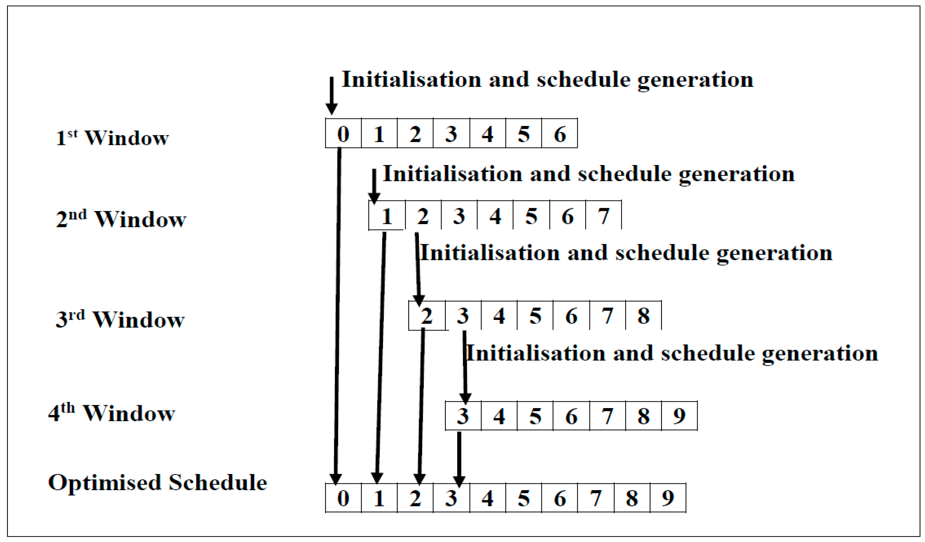
3. Dynamic RID Model with Sliding Time Window

In this paper, a unique dynamic relief items distribution with a sliding time window has been applied to address the challenges of uncertainty and changing information conditions after a disaster environment.

3.1. Sliding Time Window Optimisation

In a disaster environment, a multiple time period or periodic distribution model is required to support the disaster victims over a longer period [40,41]. Tolooie et al. [50] highlighted the need for a multi-period supply model, based on demand in each period, to make the distribution more effective. In this paper, the sliding time window optimisation has been applied to achieve optimal relief items distribution in each time period over a longer duration. Sliding time window optimisation covers the dynamicity regarding the selection of the optimum distribution schedule in each time period. In this proposedapproach, at the starting time slot (time period), the distribution schedule starts with an optimum distribution schedule based on the available information of the disaster region’s status, location, demand and available resources, including the heterogeneous vehicle fleet at supply points. At each time slot, the related information is updated, thus, the distribution schedules are re-optimised to cover the updated information. The basic flow diagram of the sliding window concept is presented in Figure 1. This proposed multi-time slot with a sliding window dynamic RID model will optimise the distribution schedule according to the updated information.

In the first time slot window, the optimum distribution schedule is generated based on the available information, which includes: vehicles’ availability, disaster region priority and relief resources. However, only one time slot distribution strategy does not make the distribution plan effective since the disaster survivors required longer support in disaster environments [51]. Considering this, in this sliding time window approach, optimised distribution schedules for each time slot based on the demand, route condition, priorities and available resources. In this approach, the distribution plan starts with an optimised distribution schedule which is re-optimised on the following time slot, i.e., when the window slides to the next time slot, the distribution schedules are re-optimised and rescheduled. In the re-optimisation process, updated information on resources, routes, priorities, and vehicles’ availability along with the pre-planned schedule is used to generate a new optimised distribution schedule at the next time slot.

3.2. Objective Function

Three objective functions and subjected constraints are set for the dynamic RID model. The minimisation of unmet demand for relief items at all demand regions and the minimisation of total vehicles’ travel time for the distribution and minimisation of the total cost are the objectives defined for this model. The delay factor (service time) is also considered in the cases where any vehicle distributes relief resources to more than one demand region. For this model, a duration of 30 min is set as the delay time for the relief items distribution processing time at each intermediate demand region in the transportation route. A number of variables, as listed in

Table 1. Variables and description used in the model.

Variables	Description
Nc	Total demand for relief items in disaster regions.
Vt	Vehicle tours with multiple demand regions.
rij	Assigned DRs in resource (RS) with the jth tour of to the ith vehicle, along with attributes DR; d, dx, dy.
fδd(rij)	A function that gives the partial relief items at rij demand regions.
fdx, dy(rij)	A function that returns the location of rij demand region.
Vt	The vehicle assigned for transportation.
Nv	Number of vehicles assigned in relief items scheduling.
kmax	Maximum missions planned in resource scheduling.
jxi	Executable missions of the assigned ith vehicle.
Φi	The velocity of the ith vehicle.
Ψi	Cost of the ith vehicle.
Tij	Time spent between demand regions rij−1 and rij of the ith vehicle.
Toffset	Offset time for the vehicle before starting the next journey.
RS	Routing Schedule.

, are defined to formulate the RID problem as follows:

i.

Minimisation of unmet demand for relief items (f1):

$$\mathrm{Min}\mathrm{f}1(\mathrm{RS})=\mathrm{Nc}-{{\displaystyle \sum }}_{\mathrm{i}=1}^{\mathrm{Nv}}{{\displaystyle \sum }}_{\mathrm{j}=1}^{\mathrm{jxi}}\mathrm{f}\mathsf{\delta }\mathrm{d}({\mathrm{r}}_{\mathrm{ij}}),1\le \mathrm{jxi}\le \mathrm{kmax}$$

ii.

Minimisation of total time spent (f2):

$$\mathrm{Min}\mathrm{f}2(\mathrm{RS})={{\displaystyle \sum }}_{\mathrm{i}=1}^{\mathrm{Nv}}{{\displaystyle \sum }}_{\mathrm{j}=1}^{\mathrm{jxi}}{\mathrm{T}}_{\mathrm{ij}}+30 {\ast \mathrm{nV}}_{\mathrm{t}}+{\mathrm{T}}_{\mathrm{offset}},1\le \mathrm{jxi}\le \mathrm{kmax}$$

where n is the total number of vehicle tours with multiple demand regions.

Subject to:

$$\mathrm{f}\left(\mathrm{x}\right)=\left\{\begin{array}{c} \frac{{{\displaystyle \sum }}_{\mathsf{\alpha }=1}^{\mathrm{j}}\mathrm{D}\left(\mathrm{fdx},\mathrm{dy}\left({\mathrm{r}}_{\mathrm{i},\mathrm{j}-1}\right),\mathrm{fdx},\mathrm{dy}\left({\mathrm{r}}_{\mathrm{i},\mathrm{j}}\right)\right)}{\mathsf{\Phi }\mathrm{i}}, \\ 0, \mathrm{Others}\hfill \end{array}\right.\mathrm{if}{\mathrm{r}}_{\mathrm{i},\mathrm{j}-1}\mathrm{and}{\mathrm{r}}_{\mathrm{i},\mathrm{j}}\notin \mathsf{\Phi }$$

iii.

Minimisation of total vehicles’ transportation cost (f3):

$$\mathrm{Min}\mathrm{f}3(\mathrm{RS})={{\displaystyle \sum }}_{\mathrm{i}=1}^{\mathrm{Nv}}\mathsf{\Psi }\mathrm{i}$$

In this dynamic RID model, the following assumptions are postulated:

• The geographical location of disaster regions and supply points are known.
• The total affected population of the disaster regions are known.
• Relief items demand is proportional to the population suffering in the corresponding disaster regions.
• Heterogeneous relief items are bounded in a single bundle and can be loaded into any vehicle.
• Connecting links between disaster regions and supply points along with corresponding distances are known.

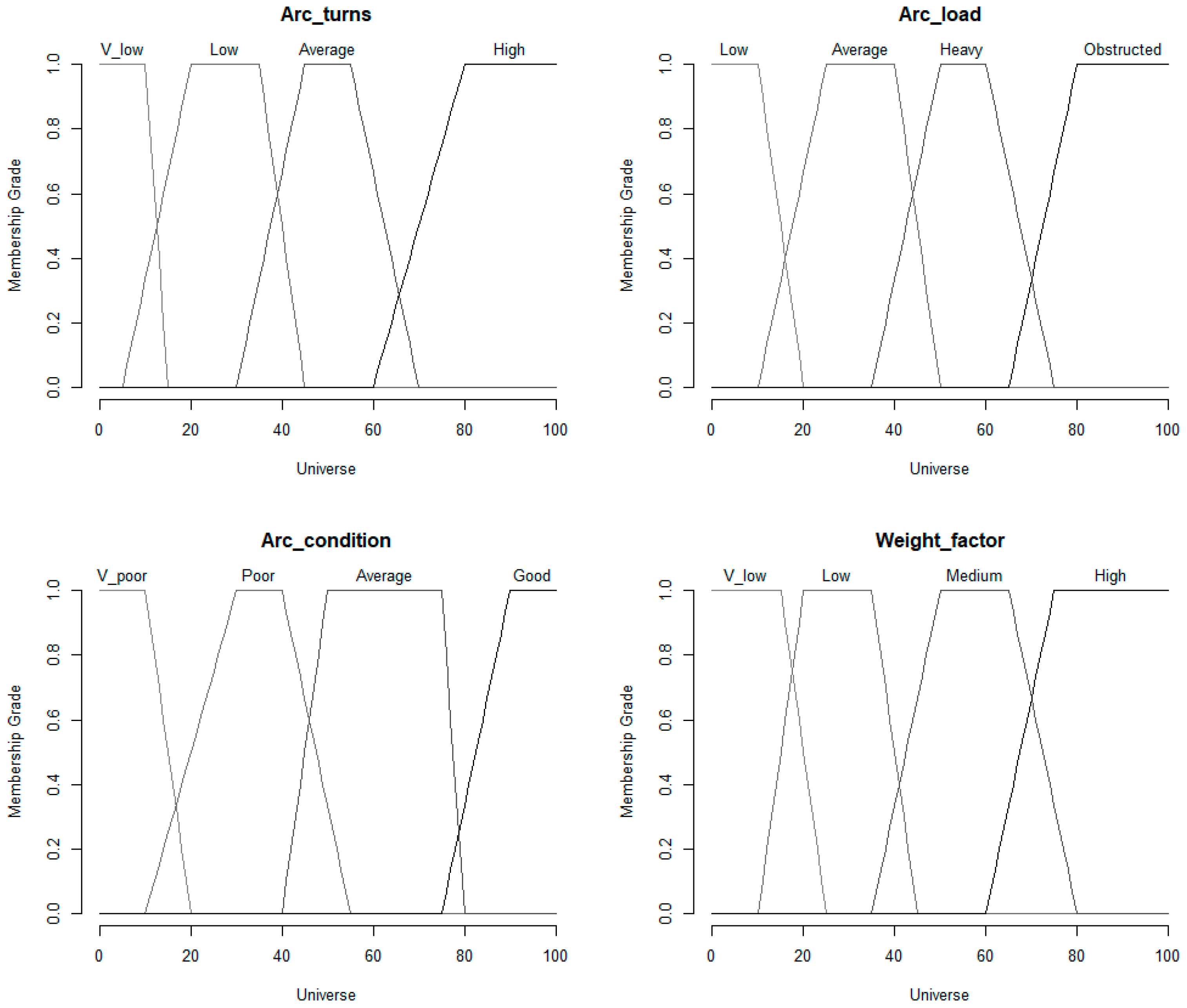
3.3. Dynamic Path Calculation Using Fuzzy Logic

In general, the shortest distance route is selected while making the selection from the supply point to the disaster region. Normally, it is assumed that the travel time is proportional to the distance between two locations. However, a disaster may damage the condition of the roads, which eventually impacts the humanitarian relief operations [52]. Therefore, due to the change in road conditions, the travel time and the selection of routes based on prior information in disaster environments may not be the optimal choice, as other factors such as road traffic condition, road geographical status, and road conditions are also crucial in defining travel time. An iterative best route selection strategy in each time slot is required based on updated information about the road conditions.

In this dynamic distribution model, a fuzzified distance matrix has been used to identify travel time more realistically. The fuzzified distance matrix is a modification of the traditional distance matrix where the crisp distances between locations are changed into the fuzzified distance. Three fuzzy input variables (Road Condition, Traffic Condition and Number of Turns) and one fuzzy output variable (Weight Factor) are used in the dynamic RID model. There has not been any sufficient appropriate data available for defining the fuzzy memberships and rules for this paper. However, there has been evidence that in the absence of sufficient data, the appropriate knowledge base is useful in defining the fuzzy system [53].

In this model, based on research works on road traffic conditions after disaster environments [54,55] and generalised knowledge from the literature, the three most appropriate fuzzy variables, values (listed in

Table 2. List of fuzzy variables and values.

Fuzzy Variables/ Values
Road Condition	Very poor	Poor	Average	Good
	[0 20]	[10 55]	[40 80]	[75 100]
Traffic Condition	Low	Average	Heavy	Obstructed
	[0 20]	[10 50]	[35 70]	[65 100]
Number of Turns	Very low	Low	Medium	High
	[0 15]	[5 45]	[30 70]	[60 100]
Weight Factor	Very low	Low	Medium	High
	[0 25]	[10 45]	[35 80]	[60 110]

) and forty fuzzy rules are defined. These fuzzy variables reflect the generalised circumstances with different levels of travel route status after the disaster. Four fuzzy levels for each fuzzy variable have been applied to describe the road status. Each of these parameters has been fuzzified with different linguistic sets. The trapezoidal membership function is selected for each input and output parameter. For each fuzzy variable, the universe is defined in the range [0 100] and the membership value in the range [0 1]. Fuzzy values are defined by their corresponding range in the universe as shown in the plot in Figure 2. These ranges are defined in terms of the condition of the fuzzy variables. For example, for Arc turns, the range [0 15] is defined as very low, range [5 45] and so on as listed in Table 2.

Appropriate fuzzy rules are synthesised considering all parameters with the relevant importance in disaster environments. Some of the synthesized rules are presented below:

Example of the Fuzzy rules

If Arc_condition = V-poor and Arc_load = Obstructed and Arc_turns = High

Then Weight_factor = V_low.

If Arc_condition = Poor and Arc_load = Average and Arc_turns = Average

Then Weight_factor = Low.

If Arc_condition = Average and Arc_load = Low and Arc_turns = V_low

Then Weight_factor = High.

If Arc_condition = Good and Arc_load = Average and Arc_turns = Average

Then Weight_factor = Medium.

If Arc_load = Average or Arc_turns = Average

Then Weight_factor = Low.

Defuzzification is applied to get a value of weight factor by applying an inferred fuzzy reasoning. The standard Centre of Gravity method is used for the approximation of the distribution of the fuzzy sets. After defuzzification, each crisp arc length in the distance matrix is changed into a fuzzified distance matrix. This fuzzified distance matrix is used to find the shortest equivalent route between any two links by applying the Floyd–Warshall algorithm as this algorithm has better performance in finding the all-pairs shortest paths in the dense graph [56]. The fuzzified distance and its impact on travel time are illustrated in the following example.

Example:

• Distance between supply point 30 to disaster region 1: 20.75 km
• Vehicle speed: 40 km per hour
• Travel Time (based on: traditional distance/vehicle speed): 31.12 min

Assume fuzzy variables as:

• Arc-Condition = Poor, Arc-Load = Heavy, Arc-Turns = High
• Arc-Weight-Factor (Applying fuzzy variables and rules): 0.357
• Effective length: 20.75 + 20.75 ∗ (1 − 0.357): 34.092 km
• (based on the synthesised fuzzy system)
• Travel Time (based on: fuzzified distance/vehicle speed): 46.68 min

From the above example, it has been clearly observed that the travel distance and, hence, the travel time is changed because of the changed condition of the routes. This signified that for an effective travel plan, all the routes’ travel time needs to be calculated as an effective travel time.

3.4. Heterogeneous Vehicles Routing (HVR)

In the dynamic relief items distribution model, a variant of the VRP considering a heterogeneous fleet with a limited number of vehicles at supply points is applied. The objective of HVR is defined to select the vehicle sets and routes from the supply points by optimising the selection criteria. In this model, the best-fit method is applied as the selection criteria for the vehicle selection at each supply point in each time slot. The best-fit selection gives the most suitable vehicle settings based on the relief item demand volume and the vehicle’s loading capacity for distribution. For the HVR, the following assumptions are applied to the constraints set:

i.

Only the disaster regions with non-negative relief demand are considered for vehicle routing at each time slot.

ii.

Thirty minutes duration is set as the delay (service) time for unloading relief items from a vehicle in a disaster region.

iii.

Additional thirty minutes duration is set as offset time for each vehicle after a round trip. This offset time is defined for vehicle refueling, cleaning and other small maintenance work. Any vehicle is available for the next trip after the roundup time with round trip journey time + service time + offset time.

For the HVP, four categories of vehicles have been considered with their cost, capacity and speed. A synthesised value on vehicle cost, capacity and speed are considered for each vehicle type as presented in

Table 3. Vehicle parameters of each type at supply points.

Parameter	Type-1	Type-2	Type-3	Type-4
Cost/Hour (£)	1000	1500	2200	3500
Capacity (kg)	4000	3000	2500	2000
Speed (kmph)	40	50	60	80

.

3.5. Priority Indexing

During post-disaster humanitarian relief task, ensuring equity in distribution to all disaster regions in a comparable way is required to enhance the effectiveness of the distribution task [6]. In some RID models, a trade-off between distribution quantitative measures in terms of distribution time, operational cost, response time and reliability have been applied by implementing rational and optimised distribution [44,57]. The study showed that response time and the number of victims, distribution time, operational cost, demand satisfaction and resource allocations are among the objectives for an effective distribution task [58]. However, with the variations in urgency levels, prioritisation of disaster areas is more important [59]. However, there has not been any unique single approach for prioritisation. Researchers have applied different approaches for defining disaster region priority, such as fuzzy clustering [43,60], multi-attribute decision-making [61] and relative priority rules using time windows [62].

The inclusion of priorities in generating distribution sequences reflects more realistic relief item distribution in disaster environments as it first delivers the relief items to the disaster regions with a higher priority. However, in doing so, the disaster regions with low priority have a long wait for relief items. With the long wait, the conditions in those regions may get worse. Therefore, a balanced distribution is required that addresses the long wait issues such that low-priority disaster regions’ wait time is within a reasonable limit. Therefore, applying wait-time priority as one of the components of deciding the priority index makes the distribution highly effective, covering the distribution of relief items to all the disaster regions over time. In this paper, two priorities: causality level priority (based on the ratio of the affected population to the total population) and wait-time priority (based on the relief item last available at the disaster region) are implemented. These two priorities are calculated for each disaster region and, hence, the weighted priority is calculated by combining the two priorities at each time slot.

Priority Index = w1 ∗ casualty factor (normalised) + w2 ∗ wait-time (normalised)

where w1 + w2 = 1.

Adjusting the weights of these two priorities is another challenge as there is no unique weight adjustment approach defined. However, research has shown that there has been a temporary adjustment of resources to the disaster regions with higher casualty [59,60,61,62,63,64,65], which shows casualty level has a higher impact on disaster management. Considering the higher importance of casualty, the weight for casualty is set with a value of 0.75 whereas the weight for wait-time is set at 0.25. Normalisation on each factor is applied in the range [0 1] where the maximum value is set to 1 and other values are divided by the corresponding maximum value. The casualty index is calculated as a ratio of the severe causality population to the total affected population in the demand regions. In general, victim conditions get worsen with time. To adjust this condition on priority, the exponential function is chosen to reflect the disaster victims’ situations with wait-time. These two priorities are combined with weight factors to evaluate priorities regarding priority index as a single weighted priority scheduling model. The sum of the three weight factors is set as 1.

3.6. Evolutionary Search

An evolutionary search is applied to find the optimised disaster regions sequence for the distribution schedule. Chromosome structure (representing each gene as a disaster region), encoding and decoding are applied as:

Coding and Decoding

In this paper, a disaster region-based representation is applied to generate a chromosome where the genes of the chromosomes describe the disaster regions sequence that needs relief from the nearest supply points. For the solution space, the greedy search strategy starts from the first gene of the chromosome with the local search where the disaster region finds the nearest supply point for the dispatch of relief items. When any vehicle tour is planned with extra relief items, the demand of the individual demand region is updated accordingly in the sequence.

A sample chromosome representation of demand sequence:

12, 19, 1, 8, 13, 4, 28, 23, 17, 20, 26, 11, 29, 6, 27, 14, 24, 22, 3, 7, 10, 25, 15, 18, 5, 9, 16, 21

For the evolutionary search, the population size is set with 60 solutions (population) for each generation. Random sequences of disaster regions are generated as parent chromosomes in the population pool at the initial state. After the first generation, the population pool is filled with solutions with multiple criteria. Elitism is used for selecting the best 10% of solutions based on distribution time and operational cost ranking from the current generation to the next generation. The remaining individuals are decided based on tournament selection. Two-point crossover with a repair is applied to avoid any possible conflict in gene exchange during the crossover. This allows removing chromosomes with the faulty gene regarding repetition of the same gene or missing any gene in the chromosome encoding. This multi-criteria population’s selection gives diversity in the population set. Different mutation rates ranging from 0.01 to 0.1 are applied during the implementation of the evolutionary algorithm. After several simulations run, a 0.05 value is set as the mutation rate for this evolutionary search. In each iteration of the evolutionary search, for each chromosome encoding, the greedy heuristic search is applied to find the nearest demand region from the selected supply source on each round of relief item scheduling-based distance matrix.

4. Computational Experiments

To design and analyse the RID models, simulation techniques have been applied to evaluate the distribution models’ effectiveness as the simulation techniques provide greater precision [66]. For the computational experiment, information is synthesised based on the case study and related parameters presented in different disaster case studies [14,67,68,69]. Disaster regions and supply point locations have been created analogous to the Chi-Chi earthquake in Taiwan [14]. The disaster region’s data such as population and travel routes are considered as it is in the case of the Chi-Chi earthquake. At first, a static distribution model is applied and analysed to justify why the dynamic RID model is required for effective relief item distribution, hence, different ways of implementation of the dynamic distribution model are considered based on information availability.

4.1. Static RID Model with Limited Vehicles

After a disaster environment, mostly, supply points have a limited number of available vehicles. Therefore, the effectiveness of the distribution plan depends on the available number of vehicles. In this model, the distribution plan is generated under the static condition to reflect the impact and benefits of a dynamic RID model in a disaster environment. The number of vehicles of each type at each supply point is synthesised. With the limited vehicles and static distribution, the available vehicles can carry relief items only to a few numbers of disaster regions.

Distribution time is calculated by applying the relation: total distance travel/vehicle speed + service time. The operational cost is calculated as vehicle cost per hour times with the number of hours the vehicle is being used. For the complete distribution schedule, total distribution time and total operational cost are calculated to measure the performance of the distribution schedule. Since the unit of time and cost are different, we applied normalisation to both time and cost. The minimum sum of the normalised distribution time and operational cost is considered the optimised distribution schedule. After 70 generations, the best distribution schedule has:

• Total distribution time: 8.60 h
• Total operational cost: £ 17,882.86

The demand status of all disaster regions after the complete distribution schedule has been analysed. It has been observed that with the utilisation of all available vehicles, all the disaster regions do not get the relief items they needed as there was only a limited number of vehicles available. Under the static condition, the simulation result showed that some of the demand regions get their demand fulfilled, some get only partial, whereas some do not get any relief items as can be observed in Figure 3. Unmet demand supply is the major limitation of this approach, which shows that static relief distribution planning with a limited number of vehicles is not an effective approach in a disaster condition. However, optimisation of distribution time and operational cost can be applied by altering the sequence of the distribution sequence. The optimisation distribution sequence finds the minimised distribution time and operational cost of the distribution of relief items with the available resources. To overcome this unmet relief item, demand in disaster region supply points need enough vehicles. However, in most disaster environments, there is always a limitation on the available number of vehicles. Therefore, a static RID model with enough vehicle conditions reflects an infeasible option in most disaster cases. This limitation reflects that the dynamic RID model is essential for relief item distribution in disaster environments.

4.2. Dynamic RID Scheduling

A dynamic scheduling model is required to generate a complete distribution sequence by re-utilising the vehicles over the period to distribute the relief items to all disaster regions. In a dynamic RID model, either static information or dynamic information can be used for the generation of the distribution schedule. Both static and changing information scenarios are analysed in the dynamic RID model. Each component is analysed in the model before applying the proposed dynamic distribution model with fuzzy travel distance, multi-priority and sliding time window.

4.2.1. Dynamic RID Scheduling with Static Information

In this dynamic RID model, static information is used to generate a complete set of distribution schedules covering the demand fulfilment across all the disaster regions. Here, the statistic information represents the situation where information updates are not considered while generating the complete distribution sequence over multiple periods to meet all the relief item demands across all the disaster regions. A limited number of heterogeneous fleet vehicles is considered. Distribution time is calculated as the summation of travel distance divided by vehicle speed, 30 min of service time for unloading items at a disaster region and an additional 30 min is considered as an offset time for a vehicle to be available for the next journey after completing a round trip. An hourly time slot is applied for dynamic scheduling; therefore, any vehicle’s next availability time is considered by rounding up to the nearest next hour after adding travel time, offset time and rest period. Normalisation on time and cost is applied while implementing optimisation on the selection of the optimum sequence since the corresponding units of time and cost are different.

4.2.2. Dynamic Scheduling with Fuzzy Distance

With the change in the road conditions after a disaster, the optimised vehicle routing under normal circumstances may not be efficient after a disaster strike. A fuzzy distance measure is implemented to find the best feasible routes in the disaster environment. In this dynamic RID model, a fuzzy distance measure is incorporated to address vehicle routing in more realistic conditions after any disaster where the distance matrix is modified into a fuzzified distance matrix to find the effective shortest path for vehicle routing. The fuzzified distance matrix is updated for each time slot with updated information on road conditions. For each time slot, the shortest route between two points is found based on fuzzified distance using the Floyd–Warshall algorithm.

4.2.3. Dynamic Scheduling with Varying Priority

To incorporate a more realistic distribution, multiple priorities are included in this dynamic RID model. Causality index and wait-time index are applied for priority setting of individual disaster regions. The causality index reflects the percentage of the population who have been severely affected by the disaster, i.e., the causality index reflects the population with high risk; whereas, the wait time is calculated by applying a timestamp at each disaster region when it gets the relief items supplied. At first, the wait-time for each disaster region is set to 0. At each time slot, the disaster region’s wait time is calculated based on the time when the region last received the relief items. Normalisation on each factor is applied in the range [0 1] where the maximum value is set to 1 and other values are divided by the corresponding maximum value.

In this model, the priority factor is calculated for each time slot as a weighted sum of casualty index and wait-time index as below:

Priority Factor = 0.75 ∗ Casualty Index (normalised) + 0.25 ∗ Wait-time Index (normalised)

Each distribution sequence is evaluated based on total distribution time, operation cost and priority factor. These three parameters are first normalised and then combined as a weighted sum to find a weighted fitness value. Based on the weighted fitness value, each distribution schedule is evaluated. The distribution schedule with the minimum weighted fitness value is selected as the best distribution schedule.

Weighted fitness value = (distribution time (normalised) + operational cost (normalised) + priority factor (normalised))/3

4.2.4. Dynamic Distribution Model with Fuzzy Travel Distance, Multi-Priority and Sliding Time Window

Several distribution models have been applied to generate the distribution schedule [67,68,69,70,71,72]. However, the major limitation of these distribution models has been the use of static information. However, disaster scenarios are dynamic, which leads to including past, current and future updates in the distribution plan [48]. Some dynamic models have been implemented for short-term demand, covering the uncertainty of demand across the disaster regions [70] and multiple stochastic periods [41], but these models are based on the estimation of the future update based on present data. The use of estimation may reduce the effectiveness of the distribution task as the actual data may be different than the estimated data. The dynamic model is only effective if regular timely updates on resources, transportation fleet and vehicle routing routes are implemented in the model [73]. An effective relief item distribution plan must be determined by considering all possible demand scenarios [74]. Relief demand, available resources and route information changes dynamically, therefore, the initial distribution plan needs to be optimised with the change in information [67]. The inclusion of simultaneous factors for disaster relief operations assists in implementing an efficient distribution plan [75].

Considering these limitations and needs, a combined dynamic RID model with fuzzy distance and multi-priority with sliding time window is applied together in the proposed model, which reflects the closest modelling of the real-time disaster environments where the decision-makers must integrate the disaster region priority and road conditions for vehicle transportation along with the changing information of each time-slot. To address the need for multiple factors in a single model, this proposed model covers the disaster conditions relief item distribution in the optimum possible way. The dynamic RID model with fuzzy travel distance, multi-priority and sliding time window generates an optimised distribution schedule at each time slot based on the information update. The optimised distribution schedule at time slot 0 is generated with the available information. With the information update at each time slot, the distribution schedule generated at the previous time slot is re-optimised.

For the computational experiment, five time slots are selected for the relief item distribution. Initial relief demand is assumed as of the Chi-Chi case study and additional demand that appears in the next time slots are synthesised as listed in

Table 4. Demand status of disaster regions at different time-slots.

	Demand
Disaster Regions	Time Slot 0	Time Slot 1	Time Slot 2	Time Slot 3	Time Slot 4
1	6500	2000	500	100	0
2	4000	500	0	100	0
3	6500	700	700	0	500
4	3800	800	1000	0	500
5	3900	1200	0	500	0
6	9800	1500	0	100	0
7	6500	900	500	200	0
8	4000	1000	0	500	0
9	6500	800	300	400	0
10	3800	1100	200	0	0
11	3900	900	1000	0	500
12	9800	1200	2000	0	0
13	6500	800	400	500	0
14	4700	700	300	0	0
15	7000	500	300	0	0
16	4800	400	200	0	0
17	4300	400	0	500	0
18	8800	500	200	200	0
19	7000	1200	500	0	0
20	3800	100	0	500	1500
21	5200	100	0	1000	0
22	8500	1000	500	1500	0
23	4200	200	0	0	500
24	8300	200	0	500	0
25	6500	100	0	500	0
26	4800	200	0	1000	1500
27	4700	200	0	600	200
28	10,800	1500	500	1500	500
29	6200	500	0	500	0

. In this table, time slot 0 lists the initial demand, and time slot 1 to time slot 4 lists the additional demand that appears across all the demand regions. Vehicle availability of each type at each time slot is synthesised as listed in

Table 5. Vehicle count of each type at supply points (S1:S4), Time Slot 0.

Supply Point	Vehicle Type 1	Vehicle Type 2	Vehicle Type 3	Vehicle Type 4
	T0/T1/T2/T3/T4	T0/T1/T2/T3/T4	T0/T1/T2/T3/T4	T0/T1/T2/T3/T4
S1	0/0/2/2/1	2/1/1/1/1	1/2/2/2/0	1/1/1/1/1
S2	2/1/1/1/0	0/0/0/0/1	1/1/2/2/0	1/1/1/1/1
S3	1/1/0/0/0	0/0/2/2/1	1/3/2/2/1	1/0/0/0/0
S4	2/1/1/1/1	1/1/2/2/1	0/0/1/1/1	1/1/1/1/0

(T0–T4).

The optimum demand sequence is found after optimising the demand sequence for 70 generations. The optimum demand sequence at Time Slot 0 shows some of the disaster regions being served at Time Slot 0 (marked with bold font) whereas other demand regions in the sequence (marked with normal font) receive relief items at another time slot, such as 1, 2 and so on. The number of disaster regions being served at time slots 1, 2 and others depends on the number of available vehicles at that particular time slot.

Best Plan Sequence (Time Slot 0): 27, 17, 11, 23, 9, 21, 16, 19, 12, 13, 18, 6, 4, 14, 26, 2, 1, 3, 25, 20, 7, 28, 10, 22, 8, 5, 15, 29, 24

The planned distribution sequence at Time Slot 0 might not be the optimum distribution sequence at Time Slots 1, 2 and so on as the demand, priority, distance matrix and available vehicles change in each time slot. Thus, re-optimisation of the distribution schedule is applied based on the available updated resource information, the priorities of each disaster region, available vehicles and route condition. The distance matrix is updated with recent information on the road’s conditions. The distribution sequences are re-optimised by applying the evolutionary algorithm for 70 generations and, hence, the new optimum distribution sequences have been generated for the distribution at Time Slot 1. It has been observed that with the updated information, the optimum distribution sequence planned at Time Slot 0 had been changed at Time Slot 1.

Best Plan Sequence (Time Slot 1): 24, 6, 12, 26, 15, 14, 27, 3, 25, 9, 29, 16, 2, 21, 10, 11, 20, 23, 5, 1, 18, 7, 28, 17, 8, 22, 13, 19, 4

Altogether, five time slots have been applied for the dynamic distribution of relief items in this paper. A sample of the optimised distribution schedule after each time slot is presented in

Table 6. Sample of distribution schedule generated by the dynamic distribution model with multi-priority, fuzzy travel distance and sliding window (Time Slot 0).

SId	DR	SP	VT	NnDR	ST	ET
1	27	4	1	-	0	1
2	27	4	2	28	0	3
3	17	3	1	-	0	3
4	17	3	7	16	0	3
5	11	1	2	-	0	3
6	11	1	4	12	0	3
7	23	4	1	-	0	1
8	23	4	4	22	0	3
9	9	1	2	-	0	1
10	9	1	3	-	0	3
11	9	2	1	-	0	1

S_Id: Schedule Id, DR: Demand Region, SP: Supply Point, VT: Vehicle Type, NnDR: Next Nearest Demand Region, ST: Start Time; ET: End Time. ET is the time (hour) when the vehicle completes its current tour.

. The optimum distribution schedule from each time slot is combined which reflects the optimised distribution plan over the period. The combined distribution schedule is as:

(Time Slot 0): 27, 17, 11, 23, 9, 21, 16, (Time Slot 1): 24, 6, 12, 26, 15, (Time Slot 2): 9, 21, 17, 20, 3, 10, 22, 8, 18, 1, (Time Slot 3): 26, 8, 4, 2, 24, 20, 18, 27, 13, 17, 15, 28, 6, 25, 29,
Best Plan Sequence (Time Slot 4): 3, 28, 23, 19, 7, 1, 11, 14, 20, 8, 5, 6, 9, 29, 2, 10, 12, 13, 18, 15, 17, 4, 22, 25, 24, 27, 16, 26, 21

The distribution schedules, listed in Table 6, describe the details of the distribution plan. For example, the schedule-1 sequence is described as: for disaster region (DR) 27, supply point (SP) 4 will supply relief items using vehicle type (VT) 1. This tour does not have an additional tour since the vehicle does not have any free space. The vehicle’s journey starts at the hour (ST) 0 and ends at the hour (ET) 1. Schedule-2 is described as DR 27 getting relief items from SP 4 using VT 2. In this schedule, an additional tour is planned since the vehicle has free space as the demand at DR 27 is less than 90% of the capacity of VT 2. The additional tour is planned for the next nearest demand region (NnDR) 28 from the DR 14. The vehicle’s journey starts at the hour (ST) 0 and ends at the hour (ET) 3. The other distribution schedules can be interpreted in the same way.

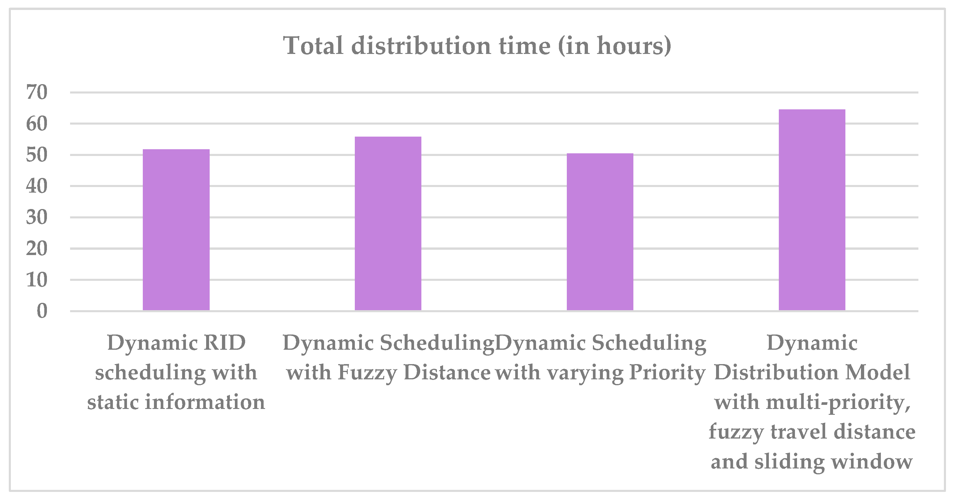
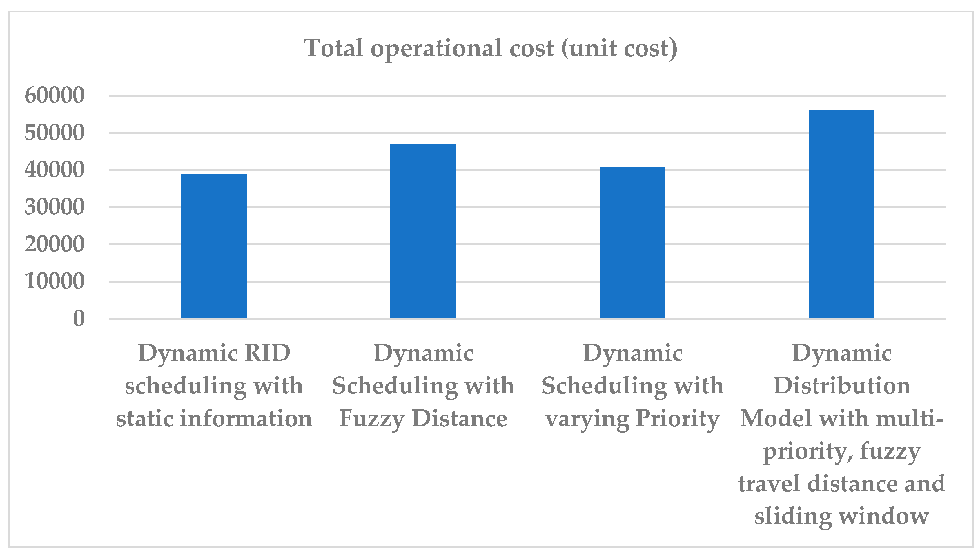
5. Comparative Performance Analysis

For the comparative analysis of the model performance, ideally the models are compared with each other by analysing performance parameters (in this case: total distribution time and total operational cost as plotted in Figure 4 and Figure 5, respectively), but the relief item distribution conditions are not same in all these models. Therefore, the simple numerical quantitative performance measure is not the best suitable option to compare the models. To evaluate the model performance, the models are compared with their feasibility, their effectiveness in the distribution of relief items and how closely the models are with the real-case disaster environments.

For the analysis, the best distribution sequence after the 70 generations is selected as a distribution plan as listed in

Table 7. Optimum distribution sequence of RID models.

Distribution Model		Demand Sequence: (Di: Disaster Regions)
Static RID model with limited vehicles		14, 2, 26, 16, 11, 4, 27, 28, 23, 5, 21, 12, 6, 1, 15, 3, 18, 17, 19, 29, 22, 25, 7,20, 10, 9,13, 8,24
Dynamic RID scheduling with static information		27, 17, 11, 23, 9, 21, 16, 19, 12, 13, 18, 6, 4, 14, 26, 2, 1, 3, 25, 20, 7, 28, 10, 22, 8, 5, 15, 29, 24
Dynamic Scheduling with Fuzzy Distance		29, 7, 25, 18, 6, 10, 23, 9, 15, 27, 5, 28, 4, 19, 22, 8, 17, 21, 1, 26, 13, 2, 14, 12, 16, 20, 3, 11, 24
Dynamic Scheduling with varying Priority		13, 4, 24, 1, 7, 29, 26, 14, 10, 8, 2, 15, 28, 3, 18, 6, 5, 21, 25, 9, 16, 22, 19, 20, 27, 11, 17, 23, 12
Dynamic Distribution Model with multi-priority, fuzzy travel distance and sliding window	Time Slot 0:	27, 17, 11, 23, 9, 21, 16, 19, 12, 13, 18, 6, 4, 14, 26, 2, 1, 3, 25, 20, 7, 28, 10, 22, 8, 5, 15, 29, 24
	Time Slot 1:	24, 6, 12, 26, 15, 14, 27, 3, 25, 9, 29, 16, 2, 21, 10, 11, 20, 23, 5, 1, 18, 7, 28, 17, 8, 22, 13, 19, 4
	Time Slot 2:	9, 21, 17, 20, 3, 10, 22, 8, 18, 1, 2, 27, 23, 13, 5, 4, 28, 25, 29, 26, 24, 19, 15, 14, 11, 7, 12, 16, 6
	Time Slot 3:	26, 8, 4, 2, 24, 20, 18, 27, 13, 17, 15, 28, 6, 25, 29, 19, 5, 21, 7, 9, 1, 11, 14, 22, 3, 12, 10, 16, 23
	Time Slot 4:	3, 28, 23, 19, 7, 1, 11, 14, 20, 8, 5, 6, 9, 29, 2, 10, 12, 13, 18, 15, 17, 4, 22, 25, 24, 27, 16, 26, 21
	Best Plan Sequence	(Time Slot 0): 27, 17, 11, 23, 9, 21, 16, (Time Slot 1): 24, 6, 12, 26, 15, (Time Slot 2): 9, 21, 17, 20, 3, 10, 22, 8, 18, 1, (Time Slot 3): 26, 8, 4, 2, 24, 20, 18, 27, 13, 17, 15, 28, 6, 25, 29, (Time Slot 4): 3, 28, 23, 19, 7, 1, 11, 14, 20, 8, 5, 6, 9, 29, 2, 10, 12, 13, 18, 15, 17, 4, 22, 25, 24, 27, 16, 26, 21

. It can be observed that the distribution sequence is not uniform. Each model generates a different optimum distribution sequence based on available resources and disaster information. These models are an effective alternative to the generated distribution schedule under different circumstances depending on the information and resources available. The static limited vehicle scheduling model is the simplest way to make a distribution plan, but with the limited vehicle condition, it may not be an effective method to distribute to all the disaster regions. To overcome the limitation of the static distribution model, dynamic RID models have been applied.

Four different dynamic models with different decision parameters have been applied. In the first dynamic RID model, a static resource information condition is used. Optimised distribution sequences, based on minimised distribution time and total operational cost, have been presented as the distribution sequence. The generation of dynamic distribution schedules maximises the use of vehicles and minimises the unmet demand. The model has a limitation as it does not have rationalised distribution in terms of covering disaster regions’ priorities, though it has the advantage of simplicity from an implementation point of view. In the second dynamic RID model, dynamic distribution schedules are generated with fuzzified road conditions. Road conditions andtraffic conditions are used to get a fuzzified equivalent travel distance. With the dynamic update on the fuzzified travel distance, the shortest travel path has also been changed dynamically. The inclusion of a fuzzified distance matrix reflects a highly realistic travel route selection in a disaster environment. However, this model does not have rationalised distribution in terms of covering priorities, which appears as a limitation of this model. The fuzzy rules are generated based on expert opinions, which is also a limitation, as expert opinions may vary.

In the third dynamic RID model, multiple priorities in terms of casualties and wait-time have been used. The priority has been calculated in each time slot with the updated information. Hence, the optimised sequences have been generated for the distribution of relief items covering multiple priorities. However, this model has a limitation in terms of static shortest path selection for vehicle transportation. The advantage of this model is that it covers heterogenous vehicles in the distribution plan along with the causality priority. In the fourth dynamic RID model, the strengths of all the discussed models are combined which makes the presented dynamic RID model as close to a disaster case of RID modelling as possible. This combined model uses fuzzified distance, multi-priorities and dynamic update with the sliding time window to generate a distribution sequence. The model starts with an optimised initial relief item distribution sequence. With updates in information, the initially planned sequence may not be the best distribution sequence in the next time slot. Therefore, the distribution sequence is re-optimised in each time slot dynamically with the updated information on disaster impact, road conditions and vehicle availability. The initial RID schedule is planned on the basis of stored information of the disaster regions in terms of population, road links and available resources. The major challenge of this model is the collection of updates in time as the information gathering after any disaster is challenging. However, it possesses the advantage that this model has the scope of any update in the next time slot during the re-optimisation of the RID schedules.

6. Conclusive Observations

Even though numerous strategies have highlighted the general relief item distribution tasks after a disaster across different cities with some limitations, the presented dynamic model covers different aspects such as disaster information updates, road conditions after the disaster, selection of the best feasible vehicles from the heterogeneous vehicles fleet and disaster region priorities, which are either missing or not properly addressed. After any disaster, these aspects reflect a realistic scenario and the inclusion of these aspects in the RID model enhances the effectiveness of the distribution task. In this paper, the aim has been to develop a dynamic RID model that reflects the realistic scenario as closely as possible after a disaster for the humanitarian supply chain as an application for smart cities. This makes the model highly practically feasible to implement for relief item distribution after a disaster. Four different theoretical and practical aspects of the dynamic RID model are highlighted, which validate why this model is a decidedly effective alternative model for the humanitarian supply chain for smart cities.

6.1. Selection of Vehicles

For the distribution task, the selection of vehicles has been one of the key components in enhancing the effectiveness of the distribution task. Many of the distribution models consider one kind of vehicle only, which is more often not the case of vehicle availability at the supply points after any disaster. Besides this, the road conditions and constraints, and relief demands also vary from one affected region to another which makes the single-type vehicles distribution plan less effective. Because of these, for the effective implementation of the relief distribution, the RID model must include the selection of vehicles from the heterogeneous vehicles fleet. The dynamic model used in this paper includes heterogeneous vehicles, which makes it a practically highly feasible option to distribute relief items. Moreover, the model applies an optimum feasible selection of vehicles based on demands across disaster regions that optimise vehicle use.

6.2. Road Conditions

The shortest route for transportation has been applied in theory and practice for many years to minimise the travel time and, hence, the response time in the disaster relief operation. However, after any disaster scenario, the road condition changes, which directly affects the travel time. Therefore, in practice, the distribution model must consider the road conditions after the disaster to make the estimation of travel time between the supply point and disaster regions more realistic. One of the practical approaches to overcoming this is to use a fuzzy variable that reflects different road conditions while finding the best feasible travel route. The dynamic model applied in this paper covered the varying road conditions, one of the major driving components in a distribution plan, to reflect a post-disaster roads condition. Fuzzified distance matrix is calculated based on road conditions to reflect the effective travel time. This inclusion of fuzzified effective distance reflects a more realistic and practical approach to finding the effective shortest distance between supply points and disaster regions.

6.3. Priority-Based Distribution

In general, the distribution models generated a distribution schedule for all the regions. The generalised distribution plan is not rational in disaster scenarios as the number of affected people and level of impact varies from one region to another. Prioritisation of the disaster regions in the distribution plan is required to support the victims who have been severely affected. One of the practical challenges in prioritisation is how to consider all the disaster regions in the distribution plan and avoid bias towards the severely affected regions. It has been observed that the condition of the less affected disaster regions worsens if there has been no relief distribution for a longer period [2]. This highlights that, in practice, any distribution model must consider the wait-time of all the disaster regions. The proposed dynamic model includes multiple priorities in terms of disaster impact severity and wait-time of all the disaster regions at all time-periods while generating the distribution schedule. This inclusion of multiple priorities makes the distribution rationalised and practically very effective, which is also very crucial in disaster conditions.

6.4. Dynamic Modelling

Over the years, several distribution models have been used aiming to achieve effective distribution. More often, those models have considered static information to generate the distribution schedule. However, the presented disaster scenarios are highly uncertain and information is not static. Therefore, the static RID models are less suitable in disaster scenarios. In practice, the dynamic models are the best-suited models as the dynamic model adopts the changing information over time and generates a distribution plan accordingly. The major advantage of the dynamic RID model is the generation of the distribution schedule with the updated information on available vehicles, other resources, road conditions and disaster region priority at any particular time slot. Combining multiple components in a single model has reflected a closer realistic condition for relief item distribution under disaster conditions. The inclusion of dynamicity in the distribution task is best suited for decision-makers in disaster relief management operations.

7. Discussion and Future Research Directions

Under a disaster environment, in any smart city, the information related to disaster impact, connecting routes and other available resources change dynamically, which has an impact on generating an optimal distribution schedule. With the emergence of the use of IoT technologies for data gathering in smart cities, the influential parameters for a RID model in a disaster environment can be updated accurately and timely. The generation of effective relief item distribution schedules with the updating information is crucial in effective relief management opearations. Robustness of relief item distribution schedules concerning uncertainty of demand, transportation link complexity and changing priorities is as equally important as other factors for relief item distribution management in a disaster environment. This uncertainty adds additional challenges to the RID management. Additionally, with the increase in the complexity of finding the best feasible transportation link for vehicle routing, the complications of effective distribution planning have increased. With the consideration of transportation link conditions and capacity in distribution planning, the presented RID model enhances the effectiveness of humanitarian supply chain management. In addtion, the RID model often lacks consideration of the priority aspects. The inclusion of multiple priorities in the presented dynamic RID model distribution schedule provides a rational distribution of relief items across all the disaster points. This rationalised distribution balances the distribution task, reflecting the effecitveness of RID management. Along with rational distribution, multi-objective and heterogeneous fleet vehicle transportation often appeared to be other challenges. These two additional aspects, multi-objective and heterogeneous fleet vehicle, have also been included to cover the more realistic scenarios of relief item distribution after any disaster. Modelling RID with heterogeneous vehicles allows to optimise the distribution time and operaional cost as the model chooses the best-fit vehicles for the relief item distribution. Often, a disaster requires a longer period of support to bring the disaster victim’s life back normal conditions. Considering this, in the presented dynamic model, multiple time slots with the updated information on disaster impact level, updated vehicle information, available resources and road condition are considered for the distribution of relief item re-optimisation of the distribution schedule at each time slot gives the mulit-period distribution as an optimised solution for a longer run as well.

With the inclusion of these major components, the presented dynamic RID model appeared as an effective model in post-disaster humanitarian supply chain management. The comparative study showed that the different models have their advantages and disadvantages. However, the presented dynamic RID model with fuzzified distance and multi-priorities with a sliding window reflected the best feasible condition that covered many of the components that have an impact on the generation of the distribution schedule. The presented dynamic models have advantages over the model used for the case study scenarios model [14] as it brings the dynamicity on disaster condition updates and available resoources to each time-period. Concerning managerial aspects, covering many disaster impact components in one model makes the disater relief operation task more effective than the traditional models. The major advantage of the presented dynamic RID model is that it starts with an initial optimised distribution schedule and re-optimised on each time slot with the updated information for all the components.

In future research, the proposed dynamic distribution model can be incorporated with real-time data collection mechanisms such as GIS mapping, satellite imaging, social media data mining and IoT sensor implementation. Use of GIS mapping and satellite imaging will help to identify the most affected disaster regions. The GIS mapping and satellite imaging information will help to set priorities for the disaster regions. Additionally, any blockages or disruptions of the transportation routes will be analysed in a more effective way to find the best feasible route for transportation. Any update on the disruption of the route can be incorporated to redefine the transportation route that is re-optimising the travel route if needed. Monitoring real-time updates on demographic information with the inclusion of these techniques will provide better mobilisation of resources at disaster regions. It can be useful for vehicle location information that can be applied to make the distribution model more dynamic. Use of GIS and satellite imaging can be used at any stage of disaster management, starting from the preparedness to the post-disaster management.

Another component that can be added to this research is the use of social media as a data source. Use of social media has increased over the years. The information available through social media will be very useful to understand the severity of the disaster. The data from social media such as Facebook and Twitter can be analysed using text mining or image mining to extract knowledge about the disaster. This knowledge can be implemented to identify disaster region priority and route conditions. Furthermore, as a future enhancement of this dynamic distribution model, IoT devices can be integrated into this dynamic relief items distribution system. The real-time update on disaster information using IoT devices can be implemented in developing the distribution schedule. The inclusion of these techniques will further enhance the effectiveness of the distribution model with the accurate and timely collection of data and making relief item distribution more effective.

References

1. Khanchehzarrin, S.; Panah, M.G.; Mahdavi-Amiri, N.; Shiripour, S. A bi-level multi-objective location-routing optimization model for disaster relief operations considering public donations. Socio-Econ. Plan. Sci. 2022, 80, 101165. [Google Scholar] [CrossRef]
2. Bozorgi-Amiri, A.; Khorsi, M. A dynamic multi-objective location–routing model for relief logistic planning under uncertainty on demand, travel time, and cost parameters. Int. J. Adv. Manuf. Technol. 2016, 85, 1633–1648. [Google Scholar] [CrossRef]
3. Holguín-Veras, J.; Taniguchi, E.; Jaller, M.; Aros-Vera, F.; Ferreira, F.; Thompson, R.G. The Tohoku disasters: Chief lessons concerning the post disaster humanitarian logistics response and policy implications. Transp. Res. Part A Policy Pract. 2014, 69, 86–104. [Google Scholar] [CrossRef] [Green Version]
4. Berariu, R.; Fikar, C.; Gronalt, M.; Hirsch, P. Understanding the impact of cascade effects of natural disasters on disaster relief operations. Int. J. Disaster Risk Reduct. 2015, 12, 350–356. [Google Scholar] [CrossRef]
5. Freire, S.; Aubrecht, C. Integrating population dynamics into mapping human exposure to seismic hazard. Nat. Hazards Earth Syst. Sci. 2012, 12, 3533–3543. [Google Scholar] [CrossRef]
6. Erbeyoğlu, G.; Bilge, Ü. A robust disaster preparedness model for effective and fair disaster response. Eur. J. Oper. Res. 2020, 280, 479–494. [Google Scholar] [CrossRef]
7. Nie, G.; Gao, J.; Su, G. Models on rapid judgment for the emergent rescue needs during earthquake–by analysis on post earthquake events. Resour. Sci. 2001, 23, 69–76. [Google Scholar]
8. Lin, A.; Wu, H.; Liang, G.; Cardenas-Tristan, A.; Wu, X.; Zhao, C.; Li, D. A big data-driven dynamic estimation model of relief supplies demand in urban flood disaster. Int. J. Disaster Risk Reduct. 2020, 49, 101682. [Google Scholar] [CrossRef]
9. Nejat, A.; Brokopp Binder, S.; Greer, A.; Jamali, M. Demographics and the Dynamics of Recovery: A Latent Class Analysis of Disaster Recovery Priorities after the 2013 Moore, Oklahoma Tornado. Int. J. Mass Emergencies Disasters 2018, 36, 23–51. [Google Scholar]
10. Singh, R.K.; Gupta, A.; Gunasekaran, A. Analysing the interaction of factors for resilient humanitarian supply chain. Int. J. Prod. Res. 2018, 56, 6809–6827. [Google Scholar] [CrossRef]
11. Setiawan, E.; Liu, J.; French, A. Resource location for relief distribution and victim evacuation after a sudden-onset disaster. IISE Trans. 2019, 51, 830–846. [Google Scholar] [CrossRef] [Green Version]
12. Pel, A.J.; Bliemer, M.C.J.; Hoogendoorn, S.P. A review on travel behaviour modelling in dynamic traffic simulation models for evacuations. Transportation 2012, 39, 97–123. [Google Scholar] [CrossRef] [Green Version]
13. Yuan, Y.; Wang, D. Path selection model and algorithm for emergency logistics management. Comput. Ind. Eng. 2009, 56, 1081–1094. [Google Scholar] [CrossRef]
14. Chang, F.-S.; Wu, J.-S.; Lee, C.-N.; Shen, H.-C. Greedy-search-based multi-objective genetic algorithm for emergency logistics scheduling. Expert Syst. Appl. 2014, 41, 2947–2956. [Google Scholar] [CrossRef]
15. Rocchi, A.; Chiozzi, A.; Nale, M.; Nikolic, Z.; Riguzzi, F.; Mantovan, L.; Gilli, A.; Benvenuti, E. A Machine Learning Framework for Multi-Hazard Risk Assessment at the Regional Scale in Earthquake and Flood-Prone Areas. Appl. Sci. 2022, 12, 583. [Google Scholar] [CrossRef]
16. Jung, D.; Tran Tuan, V.; Quoc Tran, D.; Park, M.; Park, S. Conceptual framework of an intelligent decision support system for smart city disaster management. Appl. Sci. 2020, 10, 666. [Google Scholar] [CrossRef] [Green Version]
17. Alizadeh, R.; Nishi, T.; Bagherinejad, J.; Bashiri, M. Multi-period maximal covering location problem with capacitated facilities and modules for natural disaster relief services. Appl. Sci. 2021, 11, 397. [Google Scholar] [CrossRef]
18. Rajak, S.; Vimal, K.; Arumugam, S.; Parthiban, J.; Sivaraman, S.K.; Kandasamy, J.; Duque, A.A. Multi-objective mixed-integer linear optimization model for sustainable closed-loop supply chain network: A case study on remanufacturing steering column. Environ. Dev. Sustain. 2022, 24, 6481–6507. [Google Scholar] [CrossRef]
19. Abdussalam, O.; Trochu, J.; Fello, N.; Chaabane, A. Recent advances and opportunities in planning green petroleum supply chains: A model-oriented review. Int. J. Sustain. Dev. World Ecol. 2021, 28, 524–539. [Google Scholar] [CrossRef]
20. Tirkolaee, E.B.; Sadeghi, S.; Mooseloo, F.M.; Vandchali, H.R.; Aeini, S. Application of Machine Learning in Supply Chain Management: A Comprehensive Overview of the Main Areas. Math. Probl. Eng. 2021, 2021, 1476043. [Google Scholar] [CrossRef]
21. Angarita-Zapata, J.S.; Alonso-Vicario, A.; Masegosa, A.D.; Legarda, J. A taxonomy of food supply chain problems from a computational intelligence perspective. Sensors 2021, 21, 6910. [Google Scholar] [CrossRef] [PubMed]
22. Kabra, G.; Ramesh, A.; Arshinder, K. Identification and prioritization of coordination barriers in humanitarian supply chain management. Int. J. Disaster Risk Reduct. 2015, 13, 128–138. [Google Scholar] [CrossRef]
23. Blecken, A.; Hellingrath, B.; Dangelmaier, W.; Schulz, S.F. A humanitarian supply chain process reference model. Int. J. Serv. Technol. Manag. 2009, 12, 391–413. [Google Scholar] [CrossRef]
24. Radianti, J.; Hiltz, S.R.; Labaka, L. An Overview of Public Concerns During the Recovery Period after a Major Earthquake: Nepal Twitter Analysis. In Proceedings of the 2016 49th Hawaii International Conference on System Sciences (HICSS), Koloa, HI, USA, 5–8 January 2016; pp. 136–145. [Google Scholar]
25. Paul, B.K.; Acharya, B.; Ghimire, K. Effectiveness of earthquakes relief efforts in Nepal: Opinions of the survivors. Nat. Hazards 2017, 85, 1169–1188. [Google Scholar] [CrossRef]
26. Hall, M.L.; Lee, A.C.K.; Cartwright, C.; Marahatta, S.; Karki, J.; Simkhada, P. The 2015 Nepal earthquake disaster: Lessons learned one year on. Public Health 2017, 145, 39–44. [Google Scholar] [CrossRef]
27. Ahmadi, M.; Seifi, A.; Tootooni, B. A humanitarian logistics model for disaster relief operation considering network failure and standard relief time: A case study on San Francisco district. Transp. Res. Part E Logist. Transp. Rev. 2015, 75, 145–163. [Google Scholar] [CrossRef]
28. Chaudhary, P.; Vallese, G.; Thapa, M.; Alvarez, V.B.; Pradhan, L.M.; Bajracharya, K.; Sekine, K.; Adhikari, S.; Samuel, R.; Goyet, S. Humanitarian response to reproductive and sexual health needs in a disaster: The Nepal Earthquake 2015 case study. Reprod. Health Matters 2017, 25, 25–39. [Google Scholar] [CrossRef]
29. Hu, S.; Han, C.; Dong, Z.S.; Meng, L. A multi-stage stochastic programming model for relief distribution considering the state of road network. Transp. Res. Part B Methodol. 2019, 123, 64–87. [Google Scholar] [CrossRef]
30. Leung, S.C.H.; Zhang, Z.; Zhang, D.; Hua, X.; Lim, M.K. A meta-heuristic algorithm for heterogeneous fleet vehicle routing problems with two-dimensional loading constraints. Eur. J. Oper. Res. 2013, 225, 199–210. [Google Scholar] [CrossRef]
31. Jiang, J.; Ng, K.M.; Poh, K.L.; Teo, K.M. Vehicle routing problem with a heterogeneous fleet and time windows. Expert Syst. Appl. 2014, 41, 3748–3760. [Google Scholar] [CrossRef]
32. Bettinelli, A.; Ceselli, A.; Righini, G. A branch-and-cut-and-price algorithm for the multi-depot heterogeneous vehicle routing problem with time windows. Transp. Res. Part C Emerg. Technol. 2011, 19, 723–740. [Google Scholar] [CrossRef]
33. Koç, Ç.; Bektaş, T.; Jabali, O.; Laporte, G. A hybrid evolutionary algorithm for heterogeneous fleet vehicle routing problems with time windows. Comput. Oper. Res. 2015, 64, 11–27. [Google Scholar] [CrossRef] [Green Version]
34. Xu, L.; Wang, Z.; Chen, X.; Lin, Z. Multi-Parking Lot and Shelter Heterogeneous Vehicle Routing Problem with Split Pickup Under Emergencies. IEEE Access 2022, 10, 36073–36090. [Google Scholar] [CrossRef]
35. Anuar, W.K.; Lee, L.S.; Pickl, S.; Seow, H.-V. Vehicle routing optimisation in humanitarian operations: A survey on modelling and optimisation approaches. Appl. Sci. 2021, 11, 667. [Google Scholar] [CrossRef]
36. Behrouz Afshar-Nadjafi, A.A.-N. A constructive heuristic for time-dependent multi-depot vehicle routing problem with time-windows and heterogeneous fleet. J. King Saud Univ.—Eng. Sci. 2017, 29, 29–34. [Google Scholar] [CrossRef] [Green Version]
37. Taniguchi, E.; Shimamoto, H. Intelligent transportation system based dynamic vehicle routing and scheduling with variable travel times. Transp. Res. Part C Emerg. Technol. 2004, 12, 235–250. [Google Scholar] [CrossRef]
38. Vidal, T.; Crainic, T.G.; Gendreau, M.; Prins, C. A hybrid genetic algorithm with adaptive diversity management for a large class of vehicle routing problems with time-windows. Comput. Oper. Res. 2013, 40, 475–489. [Google Scholar] [CrossRef]
39. Jeon, G.; Leep, H.R.; Shim, J.Y. A vehicle routing problem solved by using a hybrid genetic algorithm. Comput. Ind. Eng. 2007, 53, 680–692. [Google Scholar] [CrossRef]
40. Duhamel, C.; Santos, A.C.; Brasil, D.; Châtelet, E.; Birregah, B. Connecting a population dynamic model with a multi-period location-allocation problem for post-disaster relief operations. Ann. Oper. Res. 2016, 247, 693–713. [Google Scholar] [CrossRef]
41. Mahootchi, M.; Golmohammadi, S. Developing a new stochastic model considering bi-directional relations in a natural disaster: A possible earthquake in Tehran (the Capital of Islamic Republic of Iran). Ann. Oper. Res. 2018, 269, 439–473. [Google Scholar] [CrossRef]
42. Hatzakis, I.; Wallace, D. Dynamic multi-objective optimization with evolutionary algorithms: A forward-looking approach. In Proceedings of the 8th Annual Conference on Genetic and Evolutionary Computation, Seattle, WA, USA, 8–12 July 2006; pp. 1201–1208. [Google Scholar]
43. Sheu, J.-B. Dynamic relief-demand management for emergency logistics operations under large-scale disasters. Transp. Res. Part E Logist. Transp. Rev. 2010, 46, 1–17. [Google Scholar] [CrossRef]
44. Zhang, J.; Wang, Z.; Ren, F. Optimization of humanitarian relief supply chain reliability: A case study of the Ya’an earthquake. Ann. Oper. Res. 2019, 283, 1551–1572. [Google Scholar] [CrossRef]
45. Yahyaei, M.; Bozorgi-Amiri, A. Robust reliable humanitarian relief network design: An integration of shelter and supply facility location. Ann. Oper. Res. 2019, 283, 897–916. [Google Scholar] [CrossRef]
46. Tayal, A.; Singh, S.P. Formulating multi-objective stochastic dynamic facility layout problem for disaster relief. Ann. Oper. Res. 2019, 283, 837–863. [Google Scholar] [CrossRef]
47. de la Torre, L.E.; Dolinskaya, I.S.; Smilowitz, K.R. Disaster relief routing: Integrating research and practice. Socio-Econ. Plan. Sci. 2012, 46, 88–97. [Google Scholar] [CrossRef]
48. Zhou, L.; Wu, X.; Xu, Z.; Fujita, H. Emergency decision making for natural disasters: An overview. Int. J. Disaster Risk Reduct. 2018, 27, 567–576. [Google Scholar] [CrossRef]
49. Jin, S.; Jeong, S.; Kim, J.; Kim, K. A logistics model for the transport of disaster victims with various injuries and survival probabilities. Ann. Oper. Res. 2015, 230, 17–33. [Google Scholar] [CrossRef]
50. Tolooie, A.; Maity, M.; Sinha, A.K. A two-stage stochastic mixed-integer program for reliable supply chain network design under uncertain disruptions and demand. Comput. Ind. Eng. 2020, 148, 106722. [Google Scholar] [CrossRef]
51. Zhang, S.; Liu, J. Analysis and optimization of multiple unmanned aerial vehicle-assisted communications in post-disaster areas. IEEE Trans. Veh. Technol. 2018, 67, 12049–12060. [Google Scholar] [CrossRef]
52. Cheng, C.; Zhang, L.; Thompson, R.G. Reliability analysis of road networks in disaster waste management. Waste Manag. 2019, 84, 383–393. [Google Scholar] [CrossRef]
53. Deng, Z.; Jiang, Y.; Choi, K.-S.; Chung, F.-L.; Wang, S. Knowledge-leverage-based TSK fuzzy system modeling. IEEE Trans. Neural Netw. Learn. Syst. 2013, 24, 1200–1212. [Google Scholar] [CrossRef] [PubMed]
54. Hara, Y.; Kuwahara, M. Traffic Monitoring immediately after a major natural disaster as revealed by probe data–A case in Ishinomaki after the Great East Japan Earthquake. Transp. Res. Part A Policy Pract. 2015, 75, 1–15. [Google Scholar] [CrossRef]
55. Fang, S.; Wakabayashi, H. Travel time reliability for recovery activity immediately after disaster. Procedia-Soc. Behav. Sci. 2011, 20, 621–629. [Google Scholar] [CrossRef] [Green Version]
56. Singh, A.; Mishra, P.K. Performance Analysis of Floyd Warshall Algorithm vs Rectangular Algorithm. Int. J. Comput. Appl. 2014, 107, 23–27. [Google Scholar] [CrossRef]
57. Baharmand, H.; Comes, T.; Lauras, M. Managing in-country transportation risks in humanitarian supply chains by logistics service providers: Insights from the 2015 Nepal earthquake. Int. J. Disaster Risk Reduct. 2017, 24, 549–559. [Google Scholar] [CrossRef] [Green Version]
58. Safeer, M.; Anbuudayasankar, S.P.; Balkumar, K.; Ganesh, K. Analyzing Transportation and Distribution in Emergency Humanitarian Logistics. Procedia Eng. 2014, 97, 2248–2258. [Google Scholar] [CrossRef] [Green Version]
59. De Vries, H.; Van Wassenhove, L.N. Do optimization models for humanitarian operations need a paradigm shift? Prod. Oper. Manag. 2020, 29, 55–61. [Google Scholar] [CrossRef] [Green Version]
60. Sheu, J.-B. An emergency logistics distribution approach for quick response to urgent relief demand in disasters. Transp. Res. Part E Logist. Transp. Rev. 2007, 43, 687–709. [Google Scholar] [CrossRef]
61. Rezaei-Malek, M.; Torabi, S.A.; Tavakkoli-Moghaddam, R. Prioritizing disaster-prone areas for large-scale earthquakes’ preparedness: Methodology and application. Socio-Econ. Plan. Sci. 2019, 67, 9–25. [Google Scholar] [CrossRef]
62. Rabta, B.; Wankmüller, C.; Reiner, G. A drone fleet model for last-mile distribution in disaster relief operations. Int. J. Disaster Risk Reduct. 2018, 28, 107–112. [Google Scholar] [CrossRef]
63. Bitterman, N.; Zimmer, Y. Portable health care facilities in disaster and rescue zones: Characteristics and future suggestions. Prehospital Disaster Med. 2018, 33, 411–417. [Google Scholar] [CrossRef] [PubMed]
64. Oksuz, M.K.; Satoglu, S.I. A two-stage stochastic model for location planning of temporary medical centers for disaster response. Int. J. Disaster Risk Reduct. 2020, 44, 101426. [Google Scholar] [CrossRef]
65. Görmez, N.; Köksalan, M.; Salman, F.S. Locating disaster response facilities in Istanbul. J. Oper. Res. Soc. 2011, 62, 1239–1252. [Google Scholar] [CrossRef]
66. Mishra, D.; Kumar, S.; Hassini, E. Current trends in disaster management simulation modelling research. Ann. Oper. Res. 2019, 283, 1387–1411. [Google Scholar] [CrossRef]
67. Liu, Y.; Lei, H.; Wu, Z.; Zhang, D. A robust model predictive control approach for post-disaster relief distribution. Comput. Ind. Eng. 2019, 135, 1253–1270. [Google Scholar] [CrossRef]
68. Alinaghian, M.; Aghaie, M.; Sabbagh, M.S. A mathematical model for location of temporary relief centers and dynamic routing of aerial rescue vehicles. Comput. Ind. Eng. 2019, 131, 227–241. [Google Scholar] [CrossRef]
69. Özdamar, L.; Demir, O. A hierarchical clustering and routing procedure for large scale disaster relief logistics planning. Transp. Res. Part E Logist. Transp. Rev. 2012, 48, 591–602. [Google Scholar] [CrossRef]
70. Rawls, C.G.; Turnquist, M.A. Pre-positioning of emergency supplies for disaster response. Transp. Res. Part B Methodol. 2010, 44, 521–534. [Google Scholar] [CrossRef] [Green Version]
71. Najafi, M.; Eshghi, K.; Dullaert, W. A multi-objective robust optimization model for logistics planning in the earthquake response phase. Transp. Res. Part E Logist. Transp. Rev. 2013, 49, 217–249. [Google Scholar] [CrossRef]
72. Bozorgi-Amiri, A.; Jabalameli, M.S.; Mirzapour Al-e-Hashem, S.M.J. A multi-objective robust stochastic programming model for disaster relief logistics under uncertainty. OR Spectr. 2013, 35, 905–933. [Google Scholar] [CrossRef]
73. Sarimveis, H.; Patrinos, P.; Tarantilis, C.D.; Kiranoudis, C.T. Dynamic modeling and control of supply chain systems: A review. Comput. Oper. Res. 2008, 35, 3530–3561. [Google Scholar] [CrossRef]
74. Chang, M.-S.; Tseng, Y.-L.; Chen, J.-W. A scenario planning approach for the flood emergency logistics preparation problem under uncertainty. Transp. Res. Part E Logist. Transp. Rev. 2007, 43, 737–754. [Google Scholar] [CrossRef]
75. Liu, Y.; Cui, N.; Zhang, J. Integrated temporary facility location and casualty allocation planning for post-disaster humanitarian medical service. Transp. Res. Part E Logist. Transp. Rev. 2019, 128, 1–16. [Google Scholar] [CrossRef]
Figure 1. Sliding Time Window Approach.
Applsci 12 08358 g001
Figure 2. The plot of fuzzy variables with linguistic sets.
Applsci 12 08358 g002
Figure 3. Demand supply status across all the disaster regions with Static RID Model.
Applsci 12 08358 g003
Figure 4. Distribution time plots of different dynamic RID Models.
Applsci 12 08358 g004
Figure 5. Operational cost plots of different dynamic RID Models.
Applsci 12 08358 g005