
Identifying Coastal Wetlands Changes Using a High-Resolution Optical Images Feature Hierarchical Selection Method

Abstract
:1. Introduction
2. Materials
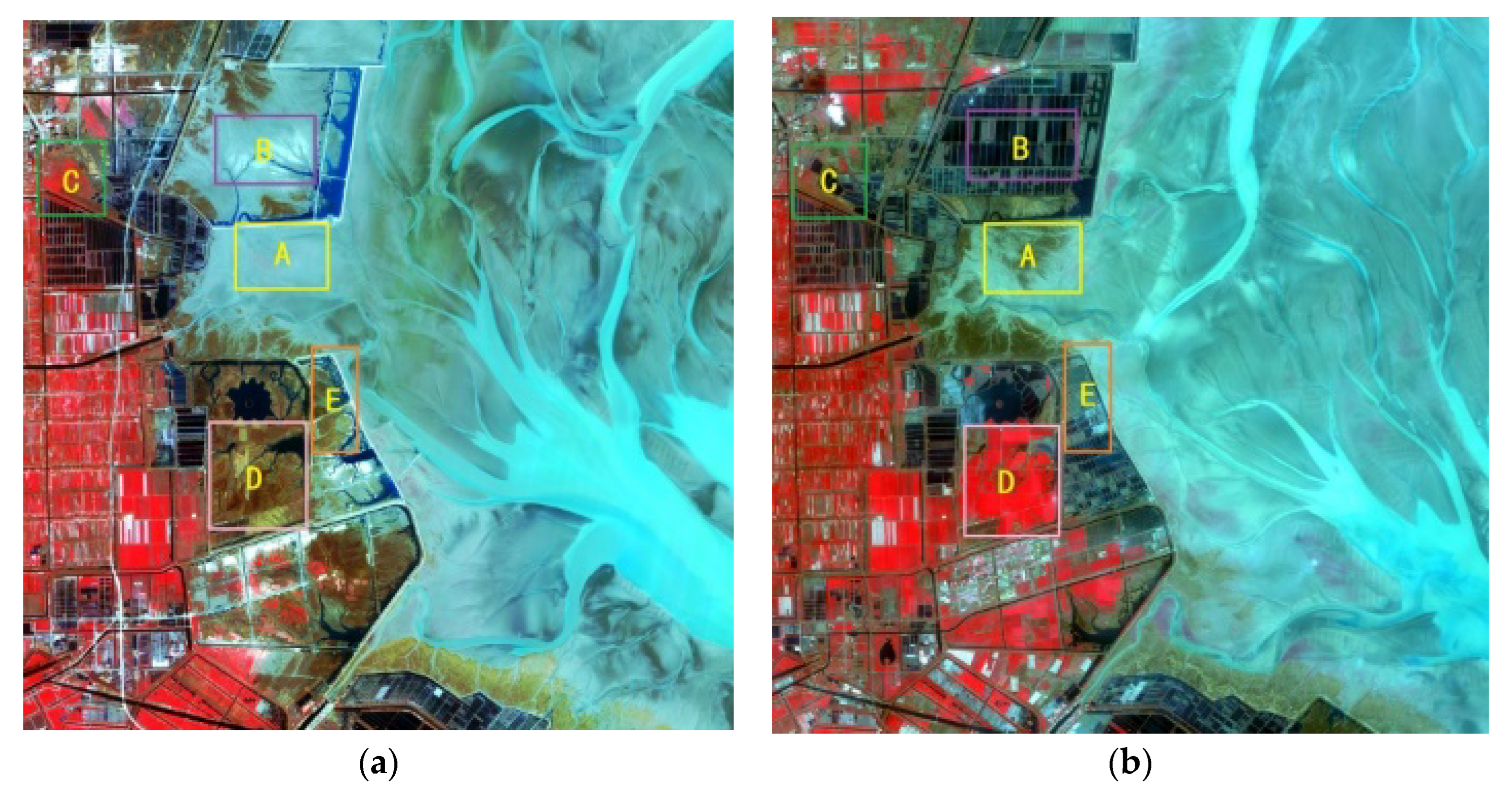
2.1. Study Area
2.2. Dataset
3. Methods
3.1. Feature Extraction
- (a)
- Spectral-based features contained five spectral features (blue, green, red, near-infrared bands, and brightness).
- (b)
- Texture-based features were GLCM (gray-level co-occurrence matrix)-based features, including mean, variance, homogeneity, dissimilarity, contrast, entropy, angular second moment, and correlation. GLCM-based textures were influenced by the window size of images, so six different window sizes, 3 × 3, 7 × 7, 11 × 11, 15 × 15, 19 × 19, and 23 × 23, were chosen to calculate GLCM textures. For four spectral bands (blue, green, red, and near-infrared band), 192 GLCM-based textures were extracted.
- (c)
- Morphological profiles (MPs) and differential morphological profiles (DMPs) can express the morphological characteristics of land cover, so the opening and closing of both MPs and DMPs were used to extract the morphological-based features. Five different scales [1,2,3,4,5] were chosen to describe the morphological characteristics on a fine to coarse scale. Eighty morphological-based features were extracted from four spectral bands.
- (d)
- Transform-based features were extracted using non-subsampling shearlet transform (NSST). NSST decomposition was used to obtain high-frequency sub-bands and low-frequency sub-bands, and NSST reconstruction was used to reconstruct image features. In order to describe the above features on a coarse to fine scale, NSST reconstruction was used on three different scales, to obtain twelve transform-based features for four spectral bands.
- (e)
- Sobel operator was used to obtain four edge-based features for four spectral bands.
- (f)
- Ten vegetation indexes (NDVI, NDWI, GR, DVI, RVI, SAVI, OSAVI, MSAVI, PVI, and EVI) were also extracted from four spectral bands, the formula of these vegetation indexes is listed in Table 2.
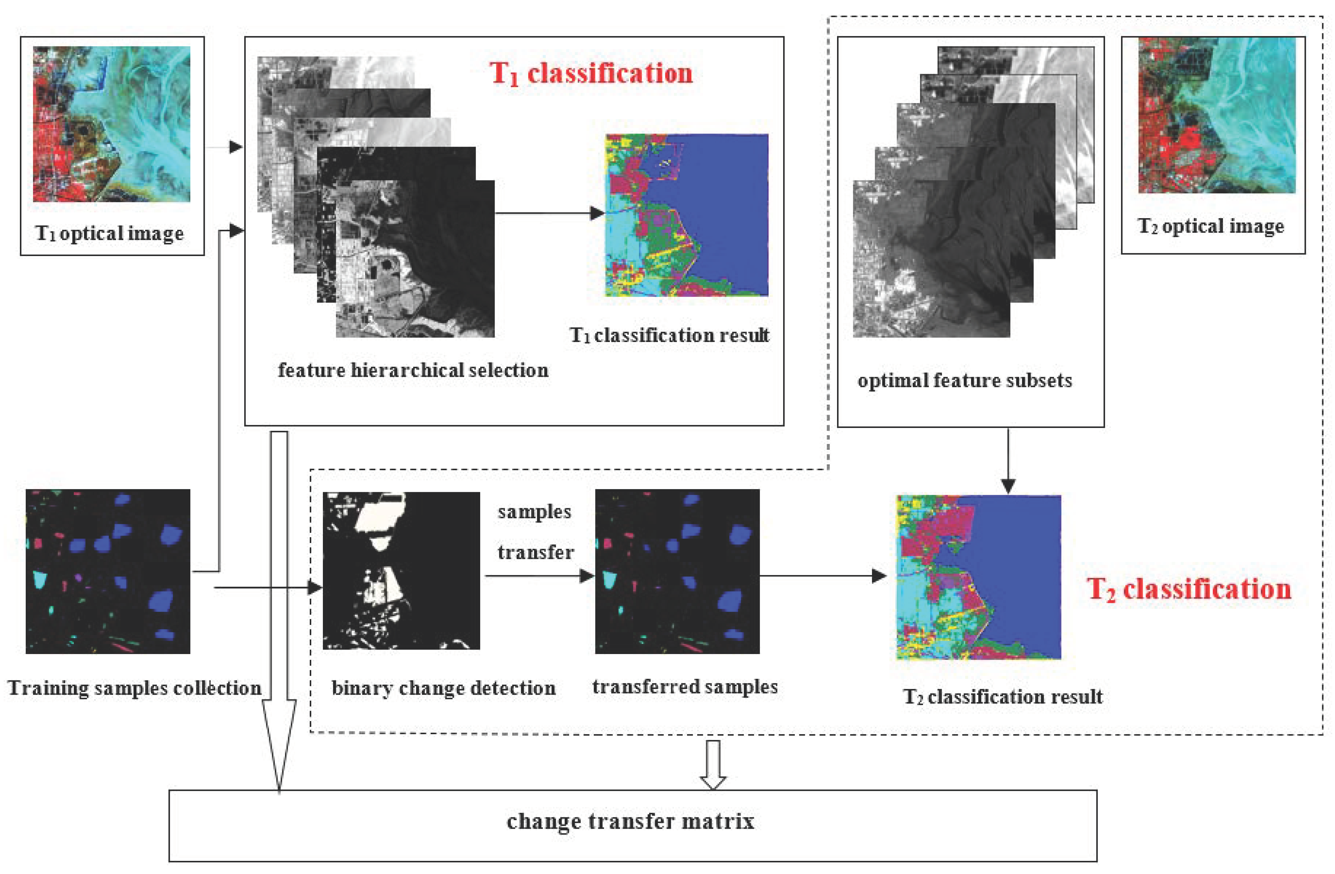
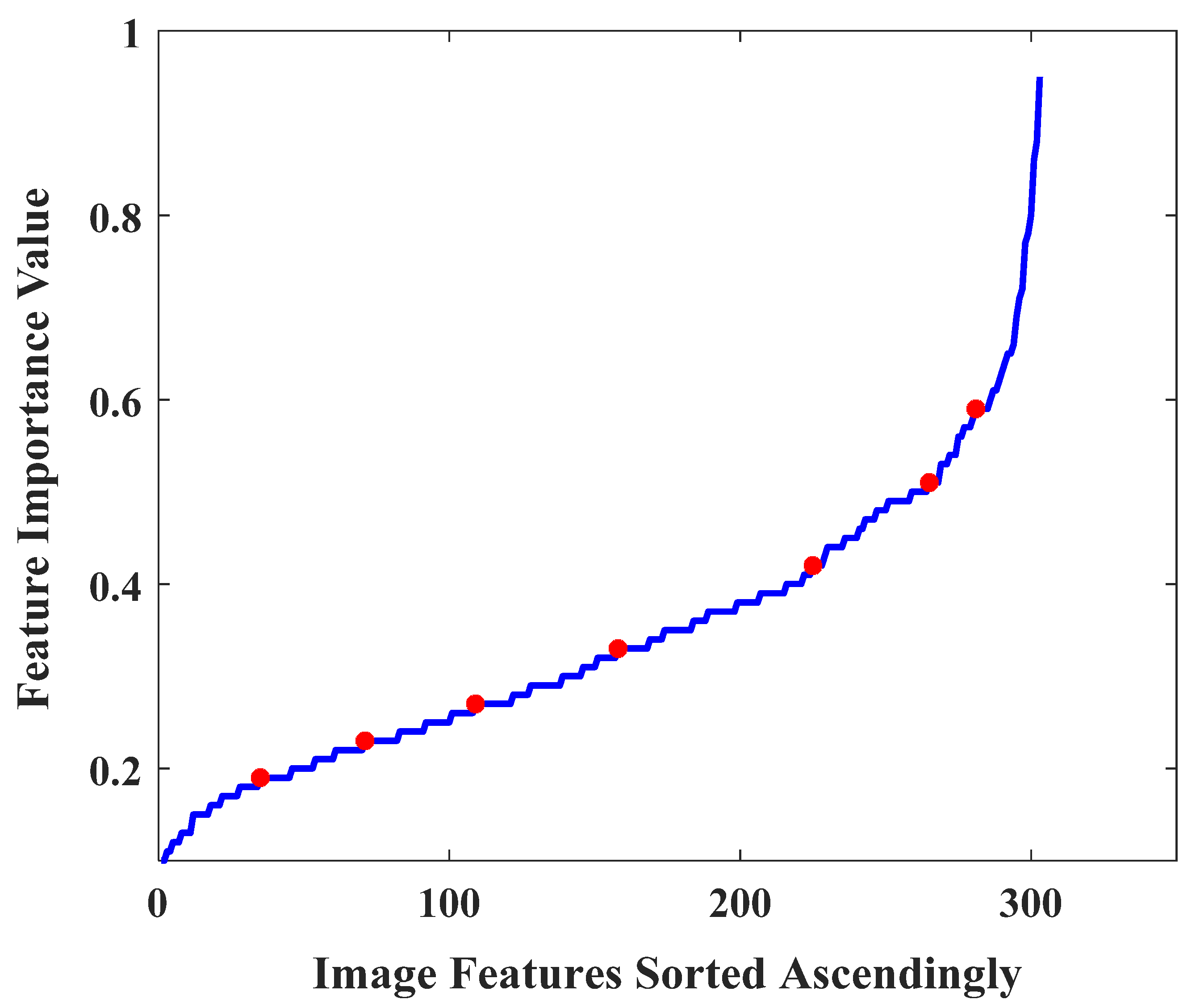
3.2. Feature Hierarchical Selection
3.3. Saliency-Guided Binary Change Detection
3.4. Change Identification Using Sample Transfer Learning
4. Results
4.1. Feature Selection Results
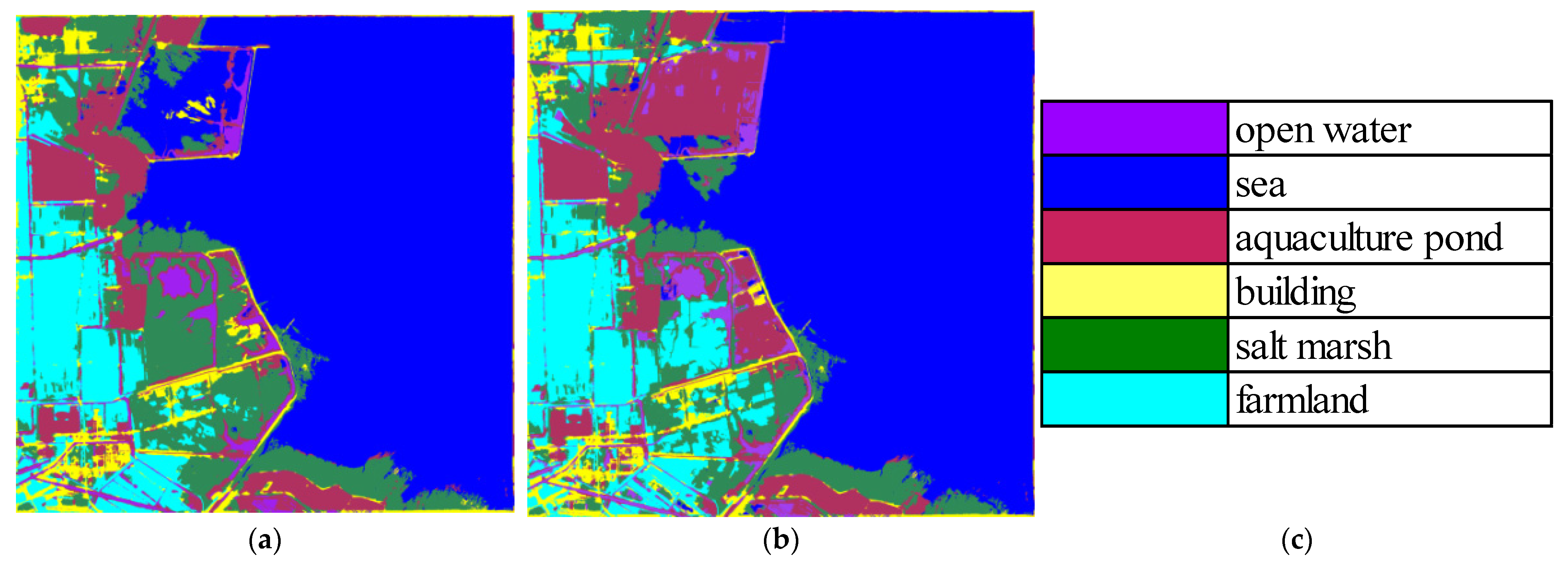
4.2. Change Identification Results
5. Conclusions
- (1)
- The jumping degree was introduced to design a feature hierarchical strategy in order to obtain optimal feature subsets. The feature selection results showed that the feature hierarchical selection method could provide a quantitative reference for optimal feature subsets selection.
- (2)
- The training samples transfer learning strategy was used to classify post-changed optical data without recollecting training samples. It could obviously save the effort of collecting training samples. The overall accuracy of the transferred training samples was 91.16%, demonstrating that it could ensure the accuracy requirements for change monitoring.
- (3)
- The southeastern coastal wetlands located in Jiangsu Province were used as a study area and ZY-3 images in 2013 and 2018 were used to conduct experiments. The results demonstrated that salt marshes increased mainly from the sea area (2.27 km2) because salt marshes expand rapidly throughout coastal areas and aquaculture ponds increased from the sea area (10.58 km2) and salt marshes (5.24 km2) because of the considerable economic benefits of the aquacultural industry.
Author Contributions
Funding
Institutional Review Board Statement
Informed Consent Statement
Data Availability Statement
Acknowledgments
Conflicts of Interest
References
- Yan, X.; Niu, Z.G. Reliability evaluation and migration of wetland samples. IEEE J. Sel. Top. Appl. Earth Obs. Remote Sens. 2021, 14, 8089–8099. [Google Scholar] [CrossRef]
- Yang, R.M.; An, R.; Wang, H.L.; Chen, Z.X.; Quaye-ballard, J. Monitoring wetland changes on the source of the three open waters from 1990 to 2009, Qinghai, China. IEEE J. Sel. Top. Appl. Earth Obs. Remote Sens. 2013, 6, 1817–1824. [Google Scholar] [CrossRef]
- Battaglia, M.J.; Banks, S.; Behnamian, A.; Bourgeau-Chavez, L.; Brisco, B.; Corcoran, J.; Chen, Z.H.; Huberty, B.; Klassen, J.; Knight, J.; et al. Multi-source EO for dynamic wetland mapping and monitoring in the Great Lakes Basin. Remote Sens. 2021, 13, 599. [Google Scholar] [CrossRef]
- Kandus, P.; Minotti, P.G.; Morandeira, N.S.; Grimson, R.; Trilla, G.G.; Gonzalez, E.B.; San Martin, L.; Gayol, M.P. Remote sensing of wetlands in South America: Status and challenges. Int. J. Remote Sens. 2018, 39, 993–1016. [Google Scholar] [CrossRef]
- Araya-Lopez, R.A.; Lopatin, J.; Fassnacht, F.E.; Hernandez, H.J. Monitoring Andean high altitude wetlands in central Chile with seasonal optical data: A comparison between Worldview-2 and Sentinel-2 Imagery. ISPRS J. Photogramm. Remote Sens. 2018, 145, 213–224. [Google Scholar] [CrossRef]
- Zhang, A.Z.; Sun, G.Y.; Ma, P.; Jia, X.P.; Ren, J.C.; Huang, H.; Zhang, X.M. Coastal wetland mapping with Sentinel-2 MSI imagery based on gravitational optimized multilayer perceptron and morphological attribute profiles. Remote Sens. 2019, 11, 952. [Google Scholar] [CrossRef]
- Sun, C.; Liu, Y.X.; Zhao, S.S.; Zhou, M.X.; Yang, Y.H.; Li, F.X. Classification mapping and species identification of salt marshes based on a short-time interval NDVI time-series from HJ-1 optical imagery. Int. J. Appl. Earth Obs. Geoinf. 2016, 45, 27–41. [Google Scholar] [CrossRef]
- Muro, J.; Strauch, A.; Fitoka, E.; Tompoulidou, M.; Thonfeld, F. Mapping wetland dynamics with SAR-based change detection in the cloud. IEEE Geosci. Remote Sens. Lett. 2019, 16, 1536–1539. [Google Scholar] [CrossRef]
- White, L.; Brisco, B.; Dabboor, M.; Schmitt, A.; Pratt, A. A collection of SAR methodologies for monitoring wetlands. Remote Sens. 2015, 7, 7615–7645. [Google Scholar] [CrossRef]
- Gao, F.; Dong, J.Y.; Li, B.; Xu, Q.Z.; Xie, C. Change detection from synthetic aperture radar images based on neighborhood-based ratio and extreme learning machine. J. Appl. Remote Sens. 2016, 10, 046019. [Google Scholar] [CrossRef]
- Xing, H.Q.; Zhu, L.Y.; Hou, D.Y.; Zhang, T. Integrating change magnitude maps of spectrally enhanced multi-features for landcover change detection. Int. J. Remote Sens. 2021, 42, 4284–4308. [Google Scholar] [CrossRef]
- Cai, L.P.; Shi, W.Z.; Hao, M.; Zhang, H.; Gao, L.P. A multi-feature fusion-based change detection method for remote sensing images. J. Indian Soc. Remote Sens. 2018, 46, 2015–2022. [Google Scholar] [CrossRef]
- Song, M.; Zhong, Y.F.; Ma, A.L. Change detection based on multi-feature clustering using differential evolution for Landsat imagery. Remote Sens. 2018, 10, 1664. [Google Scholar] [CrossRef]
- Zhao, J.X.; Liu, S.W.; Wan, J.H.; Yasir, M.; Li, H.Y. Change detection method of high resolution remote sensing image based on D-S evidence theory feature fusion. IEEE Access 2021, 9, 4673–4687. [Google Scholar] [CrossRef]
- Peng, D.F.; Zhang, Y.J. Object-based change detection from satellite imagery by segmentation optimization and multi-features fusion. Int. J. Remote Sens. 2017, 38, 3886–3905. [Google Scholar] [CrossRef]
- Wu, J.Z.; Li, B.; Ni, W.P.; Yan, W.D. An adaptively weighted multi-feature method for object-based change detection in high spatial resolution remote sensing images. Remote Sens. Lett. 2020, 11, 333–342. [Google Scholar] [CrossRef]
- Chen, Q.; Chen, Y.H.; Jiang, W.G. Genetic particle swarm optimization based feature selection for very-high-resolution remotely sensed imagery object change detection. Sensors 2016, 16, 1204. [Google Scholar] [CrossRef]
- Morchid, M.; Dufour, R.; Bousquet, P.M.; Linarès, G.; Torres-Moreno, J.M. Feature selection using principal component analysis for massive retweet detection. Pattern Recogn. Lett. 2014, 49, 33–39. [Google Scholar] [CrossRef]
- Yao, D.J.; Yang, J.; Zhan, X.J.; Zhan, X.R.; Xie, Z.Q. A novel random forests-based feature selection method for microarray expression data analysis. Int. J. Data Min. Bioin. 2015, 13, 84–101. [Google Scholar] [CrossRef]
- Chen, Y.Y.; He, X.F.; Xu, J.; Zhang, R.C.; Lu, Y.Y. Scattering feature set optimization and polarimetric SAR classification using object-oriented RF-SFS algorithm in coastal wetlands. Remote Sens. 2020, 12, 0407. [Google Scholar] [CrossRef]
- Wang, X.; Liu, S.C.; Du, P.J.; Liang, H.; Xia, J.S.; Li, Y.F. Object-based change detection in urban areas from high spatial resolution images based on multiple features and ensemble learning. Remote Sens. 2018, 10, 0276. [Google Scholar] [CrossRef]
- Xiang, S.; Xie, Q.Q.; Wang, M. Semantic segmentation for remote sensing images based on adaptive feature selection network. IEEE Geosci. Remote Sens. Lett. 2022, 19, 1–5. [Google Scholar] [CrossRef]
- Sun, C.; Li, J.L.; Liu, Y.X.; Liu, Y.C.; Liu, R.Q. Plant species classification in salt marshes using phenological parameters derived from Sentinel-2 pixel-differential time-series. Remote Sens. Environ. 2021, 256, 112320. [Google Scholar] [CrossRef]
- Bovolo, F.; Marchesi, S.; Bruzzone, L. A Framework for automatic and unsupervised detection of multiple changes in multitemporal images. IEEE Trans. Geosci. Remote Sens. 2012, 50, 2196–2212. [Google Scholar] [CrossRef]
- Shao, P.; Shi, W.Z.; He, P.F.; Hao, M.; Zhang, X.K. Novel approach to unsupervised change detection based on a robust semi-supervised FCM clustering algorithm. Remote Sens. 2016, 8, 264. [Google Scholar] [CrossRef]
- Zhuang, H.F.; Tan, D.; Deng, K.Z.; Yao, G.B. Adaptive generalized likelihood ratio test for change detection in SAR images. IEEE Geosci. Remote Sens. Lett. 2020, 17, 416–420. [Google Scholar] [CrossRef]
- Su, L.Z.; Gong, M.G.; Zhang, P.Z.; Zhang, M.Y.; Liu, J.; Yang, H.L. Deep learning and mapping based ternary change detection for information unbalanced images. Pattern Recogn. 2017, 66, 213–228. [Google Scholar] [CrossRef]
- Tewkesbury, A.P.; Comber, A.J.; Tate, N.J.; Lamb, A.; Fisher, P.F. A critical synthesis of remotely sensed optical image change detection techniques. Remote Sens. Environ. 2015, 160, 1–14. [Google Scholar] [CrossRef]
- Hussain, M.; Chen, D.M.; Cheng, A.; Wei, H.; Stanley, D. Change detection from remotely sensed images: From pixel-based to object-based approaches. ISPRS J. Photogramm. Remote Sens. 2013, 80, 91–106. [Google Scholar] [CrossRef]
- Singh, A. Digital change detection techniques using remotely-sensed data. Int. J. Remote Sens. 1989, 10, 989–1003. [Google Scholar] [CrossRef]
- Bovolo, F.; Bruzzone, L. The time variable in data fusion: A change detection perspective. IEEE Geosci. Remote Sens. Maga. 2015, 3, 8–26. [Google Scholar] [CrossRef]
- Chen, D.; Wang, Y.F.; Shen, Z.Y.; Liao, J.F.; Chen, J.Z.; Sun, S.B. Long time-series mapping and change detection of coastal zone land use based on Google Earth Engine and multi-source data fusion. Remote Sens. 2022, 14, 1. [Google Scholar] [CrossRef]
- Wu, C.; Du, B.; Cui, X.H.; Zhang, L.P. A post-classification change detection method based on iterative slow feature analysis and Bayesian soft fusion. Remote Sens. Environ. 2017, 199, 241–255. [Google Scholar] [CrossRef]
- Tong, X.H.; Pan, H.Y.; Liu, S.C.; Li, B.B.; Luo, X.; Xie, H.; Xu, X. A novel approach for hyperspectral change detection based on uncertain area analysis and improved transfer learning. IEEE J. Sel. Top. Appl. Earth Obs. Remote Sens. 2020, 13, 2056–2069. [Google Scholar] [CrossRef]
- Sui, H.G.; Feng, W.Q.; Li, W.Z.; Sun, K.M.; Xu, C. Review of change detection methods for multi-temporal remote sensing imagery. Geomat. Inf. Sci. Wuhan Univ. 2018, 43, 1885–1898. [Google Scholar]
- Wu, R.J.; He, X.F.; Wang, J. Coastal wetlands change detection combining pixel-based and object-based methods. J. Geo-Inf. Sci. 2020, 22, 2078–2087. [Google Scholar]


| Sensor | Acquisition Date | Spatial Resolution |
|---|---|---|
| ZY-3 | 4 March 2013 | 5.8 |
| ZY-3 | 22 March 2018 | 5.8 |
| Vegetation Indexes | Formula | Parameter Explanation |
|---|---|---|
| NDVI | NIR is the near-infrared band and R is the red band | |
| NDWI | G is the green band | |
| GR | B is the blue band | |
| DVI | ||
| RVI | ||
| SAVI | p is the percent of vegetation cover | |
| OSAVI | ||
| MSAVI | ||
| PVI | ||
| EVI |
| Feature Types | Image Features | Number |
|---|---|---|
| Spectral-based | blue, green, red, near-infrared bands, brightness | 5 |
| GLCM-based | mean, variance, homogeneity, dissimilarity, contrast, entropy, angular second moment, correlation | 192 |
| Morphological-based | morphological profiles (opening and closing), different morphological profiles (opening and closing) | 80 |
| Transform-based | reconstructed features using non-subsampling shearlet transform | 12 |
| Edge-based | Sobel edge feature | 4 |
| Vegetation indexes | NDVI, NDWI, GR, DVI, RVI, SAVI, OSAVI, MSAVI, PVI, EVI | 10 |
| Total | 303 |
| Different Feature Subsets | Overall Accuracy (%) | Kappa Coefficient |
|---|---|---|
| 98.36 | 0.9731 | |
| 98.51 | 0.9763 | |
| 98.17 | 0.9700 | |
| 98.24 | 0.9711 | |
| 97.99 | 0.9670 | |
| 97.59 | 0.9605 | |
| 96.57 | 0.9439 | |
| 96.07 | 0.9359 |
| 2018 | Sea | Aquaculture Pond | Salt Marsh | Farmland | Open Water | Building | Total | |
|---|---|---|---|---|---|---|---|---|
| 2013 | ||||||||
| Sea | 199.52 | 10.58 | 2.27 | 0.02 | 1.34 | 0.06 | 213.79 | |
| Aquaculture pond | 0.23 | 40.5 | 0.19 | 1.08 | 0.59 | 0.22 | 42.82 | |
| Salt marsh | 0.35 | 5.24 | 50.61 | 10.27 | 1.51 | 0.5 | 68.49 | |
| Farmland | 0.09 | 0.38 | 0.62 | 40.66 | 0.52 | 0.88 | 43.14 | |
| Open water | 0.07 | 0.93 | 0.03 | 0.04 | 10.39 | 0.03 | 11.49 | |
| Building | 0.2 | 1.34 | 0.2 | 0.36 | 0.2 | 17.96 | 20.26 | |
| Total | 200.46 | 58.98 | 53.91 | 52.44 | 14.56 | 19.65 | 400 | |
Publisher’s Note: MDPI stays neutral with regard to jurisdictional claims in published maps and institutional affiliations. |
© 2022 by the authors. Licensee MDPI, Basel, Switzerland. This article is an open access article distributed under the terms and conditions of the Creative Commons Attribution (CC BY) license (https://creativecommons.org/licenses/by/4.0/).
Share and Cite
Wu, R.; Wang, J. Identifying Coastal Wetlands Changes Using a High-Resolution Optical Images Feature Hierarchical Selection Method. Appl. Sci. 2022, 12, 8297. https://doi.org/10.3390/app12168297
Wu R, Wang J. Identifying Coastal Wetlands Changes Using a High-Resolution Optical Images Feature Hierarchical Selection Method. Applied Sciences. 2022; 12(16):8297. https://doi.org/10.3390/app12168297
Chicago/Turabian StyleWu, Ruijuan, and Jing Wang. 2022. "Identifying Coastal Wetlands Changes Using a High-Resolution Optical Images Feature Hierarchical Selection Method" Applied Sciences 12, no. 16: 8297. https://doi.org/10.3390/app12168297