1. Introduction
Production planning is a priority factor in modern manufacturing systems [
1], where a critical aspect is the scheduling of operations and resource allocation [
2]. Each industry must find a better solution for its respective production scheduling jobs to execute efficient manufacturing on time or launch new products to meet market demands satisfactorily [
3].
This paper analyses the topic of task scheduling with flexible machines, also known as the flexible job shop scheduling problem (FJSSP), especially concerning instances with high flexibility, where many machines can process the same operation. The FJSSP reflects the current problem faced by manufacturing industries in the allocation of limited but highly flexible resources to perform tasks in the shortest possible time [
4].
In the FJSSP, the goal is to find the most appropriate job sequencing, with each job involving operations with precedence restrictions, in an environment where several machines can perform the same operation but quite possibly in different processing times. Thus, the FJSSP is an NP-hard combinatorial problem where for a bigger number of jobs, there is an exponentially higher number of possible solutions [
5]. It is thus impossible to review all solutions to find the optimal scheduling in a suitable time that minimizes the processing time of all operations [
6].
Many mathematical methods have been proposed to resolve scheduling problems [
7]; some works have approached the FJSSP using the branch and bound method [
8], linear programming [
9], or Lagrangian relaxation [
10]. These methods ensure global convergence and have worked very well in solving small instances, but their computational time makes them impractical for problems with dozens of scheduling operations [
6]. That is why many researchers have chosen to move toward hybrid heuristic and metaheuristic techniques.
Over the years, distinct metaheuristic methods have been applied to solve combinatorial problems, including evolutionary algorithms using the survival of the fittest; an example is genetic algorithms (GAs) [
11,
12]. Other metaheuristics are ant colony optimization (ACO) [
13], particle swarm optimization (PSO) [
14], tabu search (TS) [
15], etc. These algorithms have been adapted to different programming problems, finding good solutions with low computational time.
The FJSSP is an extension of the classic job shop scheduling problem [
16]. In the inital problem, the optimal allocation of operations is sought on a set of fixed machines. In the FJSSP, several feasible machines can perform the same operation, often with distinct processing times.
Two problems must be considered to solve an instance of the FJSSP: the order of operations and the assignment of machines. In [
17], the FJSSP is approached heuristically, applying dispatch rules and tabu search and further introducing 15 instances with different numbers of tasks and machines. Since this work, different heuristics and metaheuristics conducting some hybrid searches have been investigated to solve this problem.
An algorithm using TS and a simplified computation of the makespan are explained in [
18], highlighting the importance of critical operations for local search. In [
19], a hybrid algorithm (HA) using GA and TS is proposed to minimize the makespan. Its model maintains a good balance between exploitation and exploration. In [
20], a multi-objective problem (MO-FJSP) is addressed applying the non-sorting genetic algorithm (NSGA-II) together with a bee evolutionary guide (BEG-NSGA-II) to minimize the makespan, the workload of the most-busy machine, and the total workload.
In [
21], a combination of genetic algorithm and a variable neighborhood descent method is shown to optimize a multi-objective version that takes into account the makespan, the total workload, and the workload of the most-busy machine, using two methods of local search. Another hybrid algorithm using the PSO and TS is presented in [
22], again for a multi-objective problem. The use of different variable neighborhoods (VNs) to refine the local search is proposed in [
23] to minimize the makespan. Another algorithm combining TS and VNs is described in [
24] for a different multi-target version of the FJSSP. In [
25], the FJSSP is studied considering maintenance costs, where a hybrid genetic algorithm (HGA) uses a local search based on simulated annealing (SA). The combination of the Harmony Search (HS) algorithm with other heuristic and random techniques is analyzed in [
26] to handle two discrete vectors, one for the sequence of operations and the other for machine allocation, to minimize makespan. Another hybrid algorithm between artificial bees and TS is presented in [
27], where the quality and diversity of solutions is rated with three metrics.
Task rescheduling is investigated in [
28], for which another hybrid technique was proposed using a two-stage artificial bee colony algorithm with three rescheduling strategies. Another hybrid method is introduced in [
29] by applying an artificial bee colony algorithm (ABC) and a TS, introducing new reprogramming processes. In [
30], a hybrid algorithm is implemented using PSO with random-restart hill-climbing (RRHC), obtaining a competitive and straightforward algorithm compared with other techniques. Another hybrid algorithm based on GA is presented in [
31] for a new specification of the FJSSP that considers the human factor as a multi-objective problem. In [
32], a PSO-GA hybrid algorithm is proposed to minimize the workload and the makespan. The minimization of inventory costs and total workflow are studied in [
33], which involves a hybrid algorithm between the ABC algorithm and the modified migrating birds optimization (MMBO) algorithm to obtain satisfactory results. Another hybrid method is put forth in [
34] based on SA and saving heuristics to minimize the energy consumption of machines, taking into account their deterioration to determine the precise processing time. In [
35], the FJSSP with fuzzy times is solved with a hybrid multi-verse optimization (HMVO) algorithm. A hybrid approach to general scheduling problems is discussed in [
36], considering batch dimensions, rework, and shelf-life constraints for defective items. The algorithm applies late acceptance hill-climbing (LAHC) and analytic procedures to accelerate the process. The computational results show the benefits of using hybridization techniques. In [
37], a two-stage GA (2SGA) is developed; the first stage is to choose the order of operations and the selection of machines simultaneously, and the second is to include new variants that avoid population stagnation. A hybrid algorithm that combines brain storming optimization (BSO) with LAHC is advanced in [
38]; the BSO is adapted to the FJSSP to explore the search space by grouping the solutions, and the exploitation is performed with the LAHC. The hybridization of the human learning optimization (HLO) algorithm and the PSO is analyzed in [
39], again applying the HLO for global search and an adaptation of the PSO to refine the local search.
The above-mentioned works suggest that hybrid approaches are still a developing research trend in solving the FJSSP and its variants, for which many of these works use GA in conjunction with another technique for local search.
However, to our knowledge, no work has applied GA operators based on a cellular automata-inspired neighborhood to explore solutions and their hybridization with the RRHC for the refinement of these solutions.
This article proposes a new hybrid technique called GA-RRHC that combines two metaheuristic techniques: the first for global search using genetic algorithm (GA) operators and a neighborhood based on concepts of cellular automata (CA) used mostly on the programming of the order of operations. As a second step, each solution is refined by a local search that applies random-restart hill-climbing (RRHC), in particular, to make the best selection of machines for critical operations, which is more convenient for problems with high flexibility. Restart is used as a simple strategy to avoid premature convergence of solutions.
The contribution of this research lies in the original use of two types of easy-to-implement operators to define a robust hybrid technique that finds satisfactory solutions to instances of the FJSSP for minimizing the processing time of all the jobs (or makespan). The GA-RRHC was implemented in Matlab and is available on Github
https://github.com/juanseck/GA-RRHC (accessed on 5 August 2022).
The structure of this article is as follows:
Section 2 provides the formal presentation of the FJJSP.
Section 3 proposes the new GA-RRHC method explaining the genetic operators used, the CA-inspired neighborhood for the evolution of the population of solutions, and the operation of the RRHC to refine each solution.
Section 4 discusses the parameter adjustment of the GA-RRHC, the comparison with six other recently published algorithms in four FJSSP datasets commonly used in the literature, making a statistical analysis based on the non-parametric Friedman test and the ranking by the relative percentage deviation (RPD).
Section 5 gives the concluding comments of this manuscript.
2. Description of the FJSSP
The flexible job shop scheduling problem (FJSSP) consists of a set of n jobs and a set with m machines. Each job has operations . Each operation can be performed by one machine from a set of feasible machines , for and . The processing time of in is represented by , and is the total number of operations.
It is necessary to carry out all operations to complete a job, respecting the operation precedence. The FJSSP has the following conditions: (1) At the start, all jobs and all machines are available. (2) Each operation can only be performed by one machine. (3) A machine cannot be interrupted when processing an operation. (4) Every machine can perform one operation at the same time. (5) Once defined, the order of operations cannot be changed. (6) Machine breakdowns are not considered. (7) Different jobs have no precedence restrictions of operations. (8) The machines do not depend on each other. (9) The processing time includes the preparation of the machines and the transfer of operations.
One solution of an FJSSP instance includes two parts, a sequence of operations that respects the precedence constraints for each job, and the assignment of a feasible machine to each operation. The objective of this paper is to calculate the sequence of operations and the assignment of machines that minimize the makespan
, the total time needed to complete all jobs, as defined in Equation (
1).
is the time when all operations in
are completed, subject to:
In this formulation, the start time of operation
in
is
. The processing time of every operation greater than 0 is reviewed in Equation (
2). The precedence between operations of the same job is considered in Equation (
3). Equation (
4) is an assignment record of one operation to a valid machine; Equation (
5) represents that each operation is processed by only one machine. The constraint in Equation (
6) guarantees that, at any time, every machine can process only one operation.
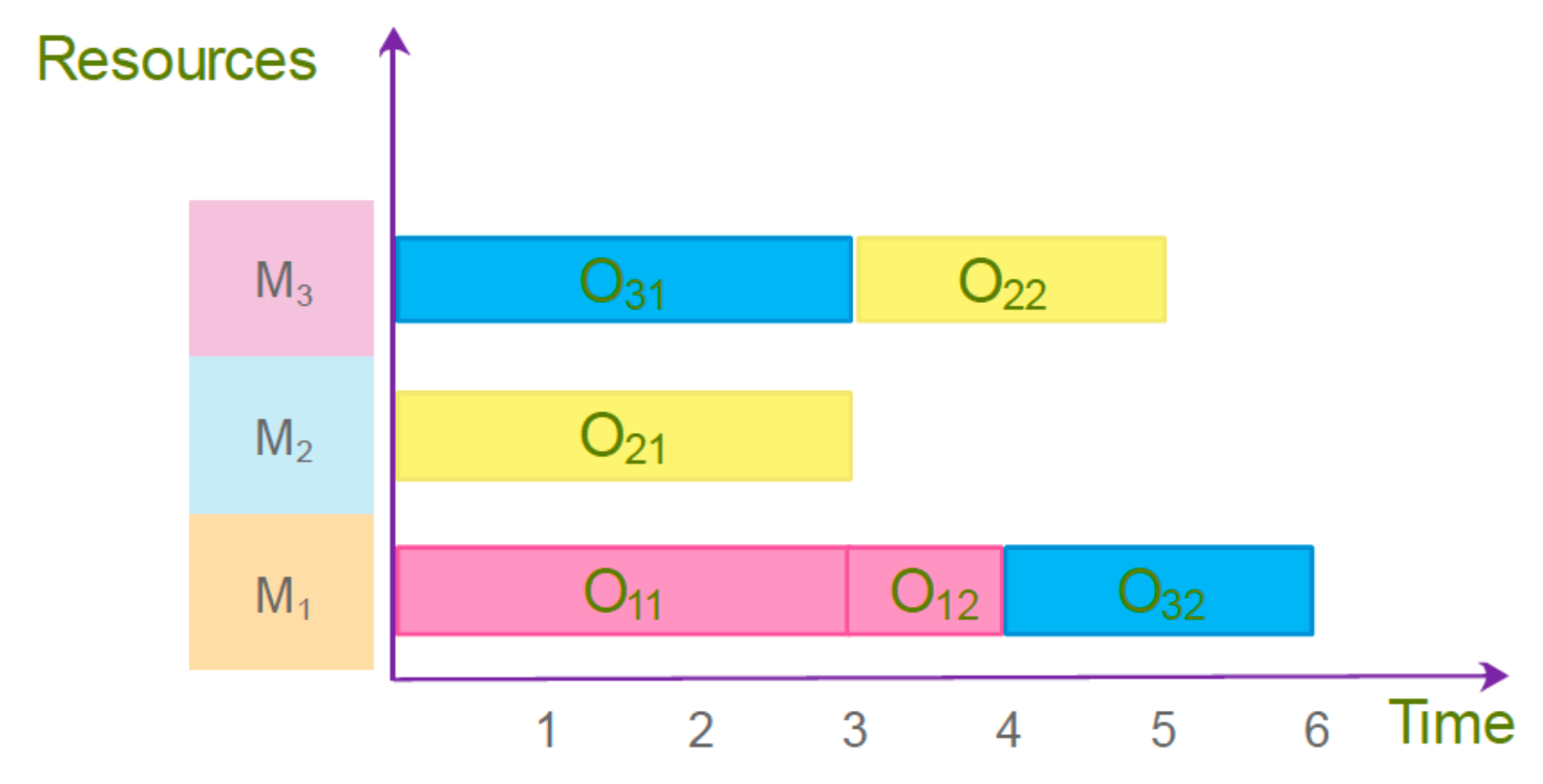
Table 1 provides an example of an FJSSP instance with three jobs, two operations per job, and three machines, where all machines can perform all operations. A possible solution to this problem is presented in the Gantt chart in
Figure 1.
3. Genetic Algorithm and Random-Restart Hill-Climbing (GA-RRHC)
The idea of using a genetic algorithm with a random-restart hill-climbing (GA-RRHC) algorithm is to propose a method that is easy to understand and implement and simultaneously capable of obtaining competitive results compared with other techniques in the optimization of different FJSSP instances.
The GA-RRHC uses a genetic algorithm as a global search method, mainly using job-based crossover (JBX) and precedence operation crossover (POX), and as mutation, the swapping of two operations and the shift of three-position jobs for the sequences of operations. Two-point crossover and mutation by changing feasible machines at random are used for machine allocation. These operators have been previously used to resolve instances of the FJSSP and have shown good [
19] results. A contribution of this work is the method of applying these operators using a neighborhood inspired by cellular automata (CA), where each solution chooses several neighbors. Crossover and mutation are applied for each neighbor, and from all the neighboring solutions, the best one replaces the original. This idea has already been explored in the global–local neighborhood search (GLNSA) algorithm, although using different operators [
40].
The local search in the GA-RRHC applies a random-restart hill-climbing (RRHC) algorithm to refine the machine selection for the critical operations of each solution. The RRHC has been used successfully in the FJSSP [
30], although not in combination with a GA, which represents another contribution of this work. An advantage of RRHC is its easy implementation, unlike other techniques for discrete problems such as simulated annealing or tabu search [
41].
In short, the GA-RRHC generates a random population of solutions. A neighborhood of new solutions produced with genetic operators is taken for each solution, and the best one is chosen. This new solution is refined with the RRHC. The optimization loop repeats until a limit of iterations is met, or a best solution is not calculated after a certain number of repetitions.
3.1. Encoding and Decoding Solutions
Initially, the GA-RRHC generates a random population of
solutions called smart-cells. Each smart-cell comprises two sequences, one for the operations (
) and the other for the machine assigned to each operation (
). Both sequences have
o elements. The GA-RRHC uses the decoding described in [
19].
In the sequence
, each job
appears
times (a permutation with repetitions). The sequence
has
o elements and is divided into
n parts. The
ith part holds the machines selected to process the job
and has as many elements as
.
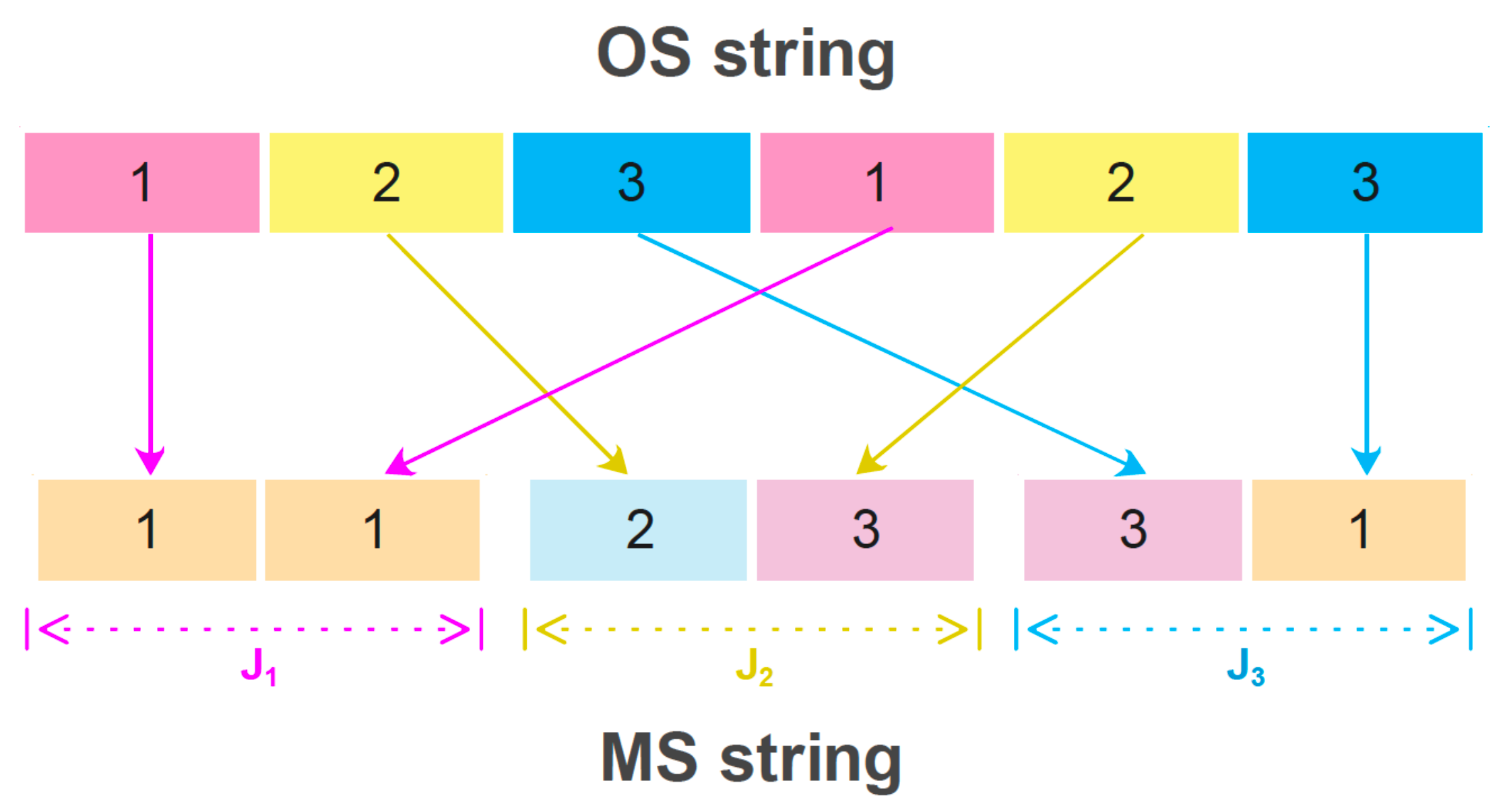
Figure 2 depicts the codification of the solution in the Gantt diagram of
Figure 1.
To decode the solution, is read from left to right. The jth occurrence of signifies that operation must be processed. This encoding allows that any permutation with repetitions represents a rightful sequence . For each part i of , the jth value represents the machine processing .
3.2. Qualitative Description of the GA
Each iteration of the GA used in this work involves a selection stage to refine the population of smart-cells, favoring those with lower makespan. Inspired by the CA neighborhood concept [
42], for each smart-cell, a neighborhood of new solutions is produced with different crossover and mutation operators. The one with the lowest makespan is chosen as the new smart-cell. The operators used for each part of the GA are described below.
3.2.1. Population Selection
Two types of selection are used in this stage: elitism and tournament. Elitism selects a proportion of the best smart-cells for the next iteration without change, guaranteeing that their information remains available to improve the rest of the population. Genetic operators and RRHC will not be applied in elite smart-cells. A tournament selection is used to select the rest of the smart-cells. Random pairs of smart-cells are chosen, and for each pair, the smart-cell with the lowest makespan is selected for the next iteration.
3.2.2. Crossover Operators
Smart-cell crossover uses two operators for
sequences, each type of crossover is applied with
probability. The first is the precedence operator (POX), where the set of jobs is divided into two random subsets
and
such that
and
. For two sequences
and
, two new sequences
and
are obtained. The operations of jobs
are placed in
in the same order as in
. The operations of
fill the empty positions of
, keeping the order from left to right (seriatim) in which they appear in
. The analogous process is carried out to form
by first taking the operations of
at the same positions as
. The empty spaces of
are filled with the operations of
in
seriatim.
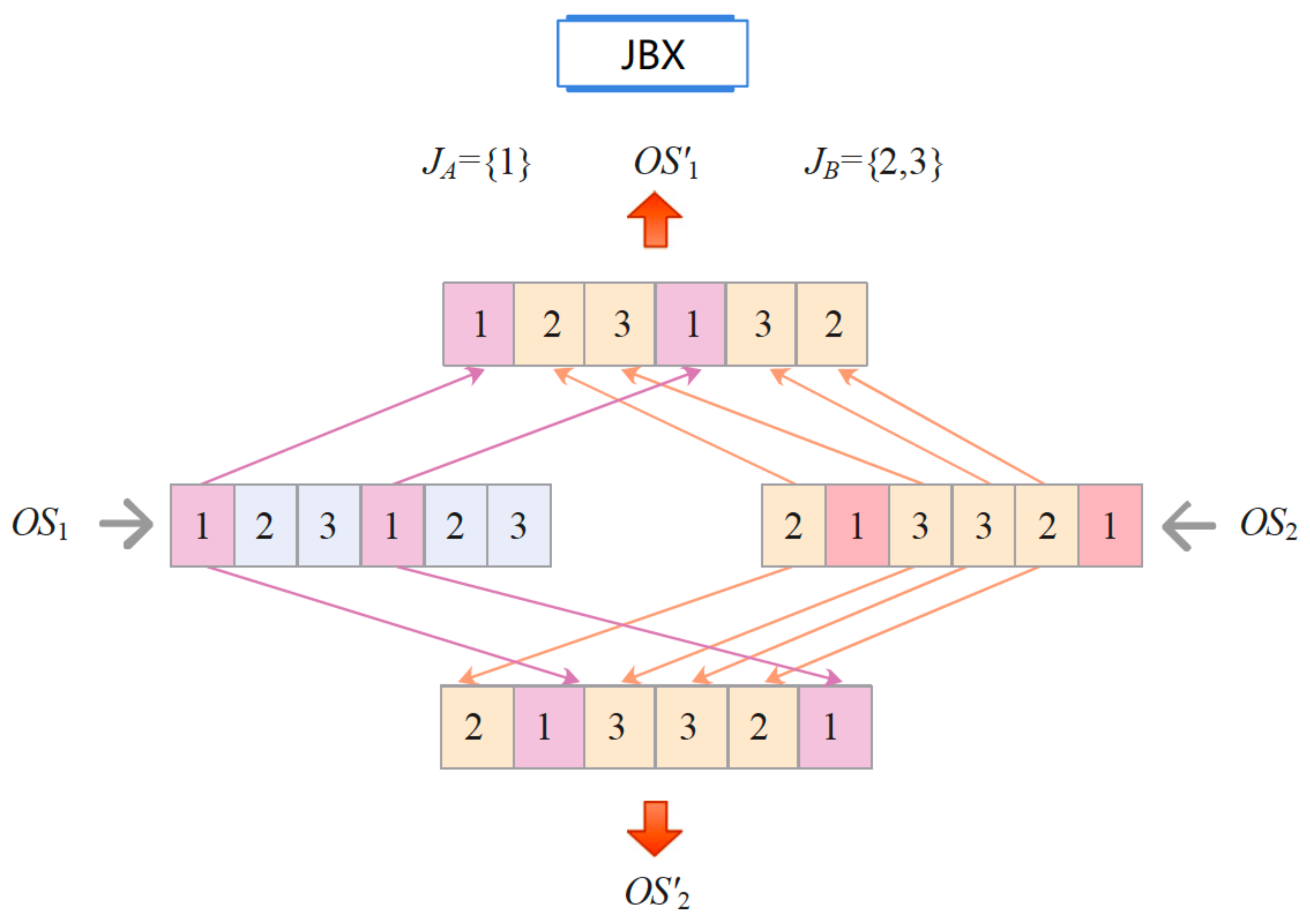
Figure 3 exemplifies the POX crossover with three jobs and six operations.
The second operator is the job-based crossover (JBX), which also defines the subsets
and
. From two sequences
and
,
is obtained in the same way. The difference lies in the specification of
, first taking the operations of
in the same positions as
. Next, the empty spaces of
are filled with the operations of
in
seriatim.
Figure 4 presents an example of a JBX crossover with three jobs and six operations.
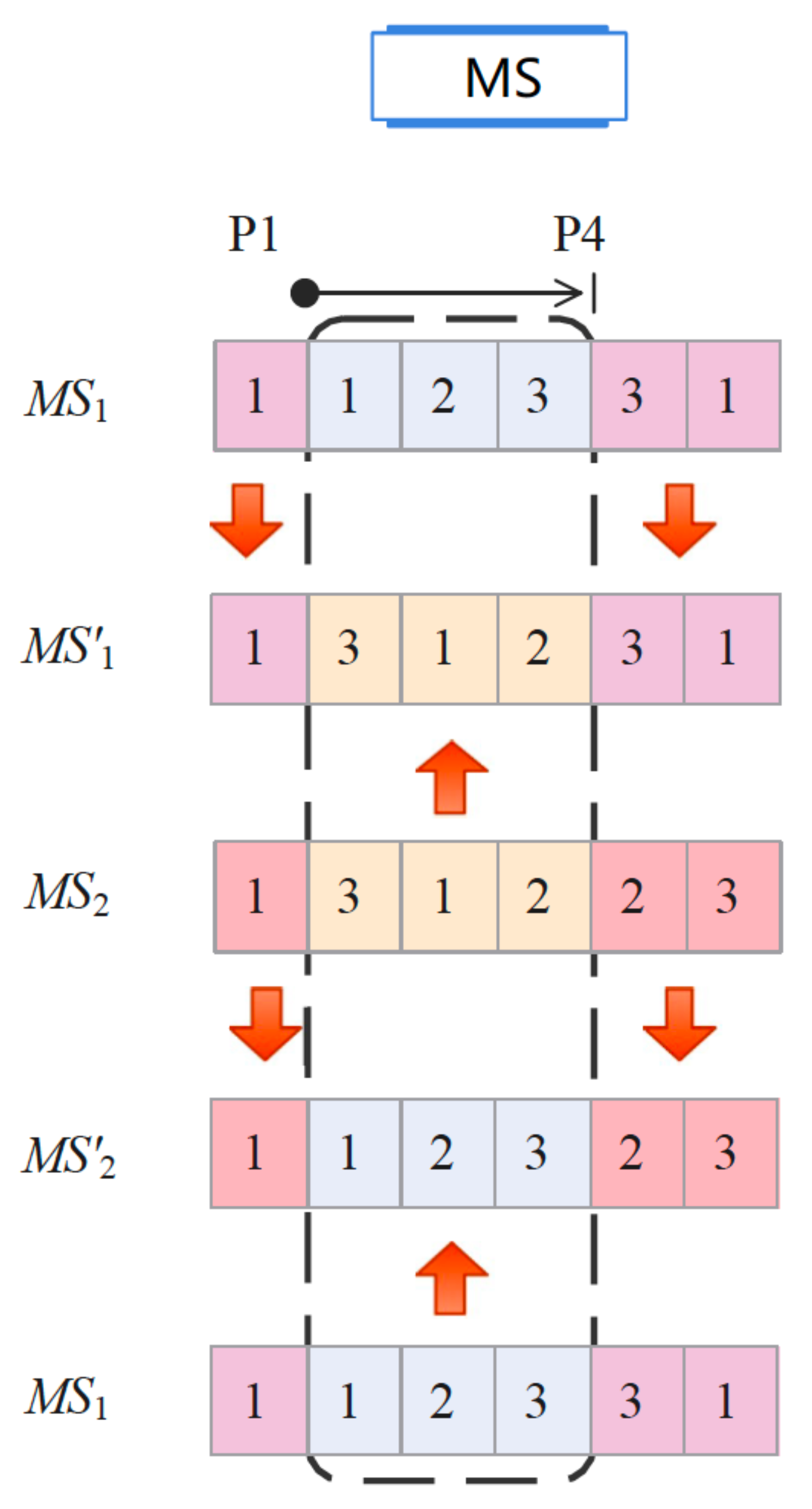
A two-point crossover is used for the sequences
. For two sequences
and
, two random positions
are chosen. A new sequence
is obtained by taking the elements of
at positions
and
and from
at positions
. Similarly, a new sequence
is formed by exchanging the roles of
and
.
Figure 5 presents a two-point cross for three machines and six operations.
3.2.3. Mutation Operators
Smart-cells mutation uses two operators over the
sequences, and each type of mutation is used with
of probability. The first is swap mutation, where two positions of
are selected and their elements swapped to obtain
. An example is in
Figure 6.
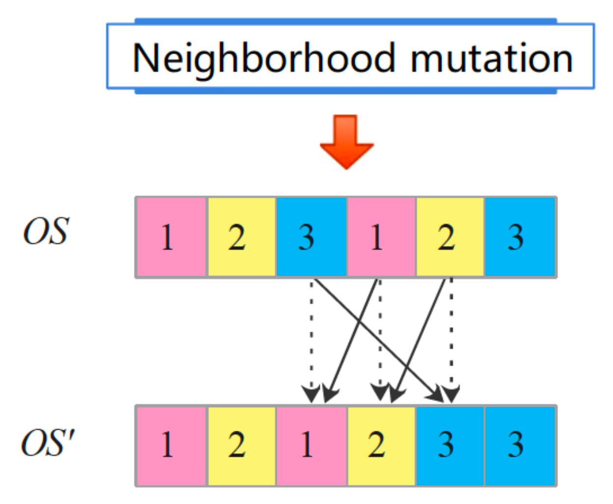
The second mutation is the random change of positions for operations of three different jobs. Three positions of
belonging to different jobs are selected and their positions randomly swapped to obtain
. Three operations from different jobs are chosen since exchanging their positions in
would not generate a new solution if the operations were from the same job. Moreover, a more significant perturbation is achieved by selecting three operations. This is suitable for the exploration stage and to escape local minima, especially in cases with a more significant number of jobs and operations. This type of mutation was proposed by [
19], obtaining good results. An example is depicted in
Figure 7.
For the sequence
, a mutation of assigned machines is applied;
random positions are chosen, and for those positions, feasible random machines, different from the initial selection, are chosen. One example is presented in
Figure 8.
3.2.4. CA-Type Neighborhood to Apply Genetic Operators
According to Eiben and Smith [
43], an evolutionary algorithm is an optimization strategy modelled around the evolution of different biological systems. If a system shows dynamic behaviors applicable in solving complex problems, it can be a source of inspiration to define new evolutionary algorithms, regardless of whether these systems are natural or artificial.
CAs are elemental discrete dynamical systems capable of generating complex global behaviors [
42,
44]. The simplest model, known as elementary CA, is discrete in states and time; it consists of a linear array of cells with an initial assigned state, which can be a number or color. Each cell keeps or changes its state depending on its present state and those of its neighbors on either side, having a whole neighborhood of three cells. This process is applied synchronously to update the state of all cells.
This CA-type neighborhood has been successfully applied in different optimization algorithms [
45,
46,
47,
48]. However, to our knowledge, this type of neighborhood has not yet been applied with genetic operators for the FJSSP. In this work, to explore the solution space, each smart-cell will generate
l new neighboring solutions using crossover and mutation. The best of these
l solutions (with the smallest makespan) is selected to update to the original smart-cell.
Figure 9 shows the CA-type neighborhood implemented in the proposed algorithm.
The previous genetic operators perform the global search mainly to improve the sequence of each smart-cell. Next, the local search method for optimizing the sequences of each smart-cell is described.
3.3. Random-Restart Hill-Climbing (RRHC)
A local search method is intended to exploit the information of the smart-cells to decrease the value of their makespan. The general idea is to start from each smart-cell and make small changes to improve the makespan. The metaheuristic used is the random-restart hill-climbing (RRHC) [
30]. The RRHC can restart the search from a solution with a makespan worse than the original one after a given number of steps to escape local minima. The whole process ends after a fixed number of steps.
The critical operations of the smart-cell are first detected to apply the RRHC. These operations define the value of the makespan, and these operations are linked by job or by a machine whose sum of processing times from the beginning to the end gives the makespan as a result, with no idle times between these operations [
18].
A record of the previous task of each operation is kept when calculating the makespan to know which are the critical operations of a smart-cell, where the initial operations of each job do not have a previous operation. This record allows a fast computation of the critical operations by simply taking one of the last operations with a completion time identical to the makespan. Subsequently, previous operations on the same machine and at the same job are analyzed, taking that with end time equal to the start time of the present operation. A random pick is made if the same completion time is held by both previous operations. The procedure is repeated until an operation with no preceding operation is reached.
Figure 10 presents the critical path of the solution represented in the Gantt diagram of
Figure 1.
From the set of critical operations, one is taken at random, and a different feasible machine is chosen to have a new sequence
. Additionally, another critical operation with probability
is selected, and is swapped with any other operation in
to have a new sequence
and generate a different solution.
Figure 11 shows a makespan improvement changing the machine assignment of a critical operation.
The RRHC is applied for iterations, having a pile of new solutions generated through the described process. If one of these solutions improves the makespan, this solution replaces the smart-cell, emptying the pile. If the makespan of the original smart-cell has not been improved after iterations, a new random solution is taken from the pile to restart the climbing. Since the RRHC focuses on improving machine allocation, it works best for instances with high flexibility.
3.4. Integration of the GA-RRHC Algorithm
Algorithm 1 depicts the GA-RRHC pseudocode.
Figure 12 illustrates the flowchart of the proposed method. After the GA-RRHC parameters are defined, the smart-cell population is generated, evaluated, and selected. GA operators are applied in a CA-like neighborhood for a global search to update every smart-cell. Next, each smart-cell is improved by a local search performed by the RRHC. Finally, the best smart-cell is returned.
| Algorithm 1: Pseudocode of the GA-RRHC |
![Applsci 12 08050 i001]() |
4. Results of Experiments
The GA-RRHC was coded in Matlab R2015a (TM) on an Intel Xeon W machine with 128 GB of RAM and running at 2.3 GHz. The source code is available on Github
https://github.com/juanseck/GA-RRHC (accessed on 5 August 2022). Four datasets were taken to test the effectiveness of the GA-RRHC. These datasets have been widely used in the specialized literature, with instances having different degrees of flexibility. A flexibility rate between 0 and 1 is specified as
= (flexibility average/number of machines). A high value of
means that the same operation can be processed by more machines.
The first experiment takes the Kacem dataset [
49], with five instances of which four have a value of
(full flexibility). The BRdata dataset is used for the second experiment and consists of 10 instances, from 10 to 20 jobs and 4 to 15 machines, with partial flexibility
[
17]. The third and fourth datasets are the Rdata and Vdata datasets, with each having 43 problems going from 6 to 30 jobs and 6 to 15 machines. The Rdata set has a maximum value of
, while all instances of the
set have a rate of
, which means that half of the machines can perform each operation [
50]. These datasets are available at
https:/people.idsia.ch/~monaldo/fjsp.html (accessed on 5 August 2022).
4.1. GA-RRHC Parameter Tuning
The GA-RRHC has nine parameters that control its operation. The total number of iterations is ; is the limit of stagnation iterations, is the number of smart-cells, is the proportion of elite smart-cells, and l is the number of neighbors of each smart-cell generated by the genetic operators. Further, is the probability of mutation of a solution, is the number of RRHC iterations, are the iterations to restart the RRHC, and is the probability of moving a critical operation in the RRHC.
For the first three parameters
, the values used in [
19,
38] were employed as a reference since these works obtained good results in minimizing the makespan. These parameter values are typically used in specialized publications and are comparable to those utilized by methods employed in the following sections to compare the performance of the GA-RRHC.
To adjust the other parameters, different levels of each parameter were taken to minimize the instance of the Vdata dataset and the best combination of parameters was chosen.
For
, the values
and
were tested, the parameter
l was tested between 2 and 3, and the values
and
were tested for
. For the RRHC, the values between 80 and 100 and between 30 and 40 were taken to tune
and
respectively. For
, the values
and
were proved. In this way, 64 different combinations of parameters were taken; for each combination, 30 independent runs were performed, selecting the set of parameters with the least average makespan.
Table 2 shows the GA-RRHC parameters to analyze its results in the rest of the instances.
4.2. Comparison with Other Methods
Six algorithms published between 2016 and 2021 were used to compare the GA-RRHC performance. These algorithms include the global–local neighborhood search algorithm (GLNSA) [
40], the hybrid algorithm (HA) [
19], the greedy randomized adaptive search procedure (GRASP) [
51], the hybrid brain storm optimization and late acceptance hill-climbing (HBSO-LAHC) [
38], the improved Jaya algorithm (IJA) [
52], and the two-level PSO (TlPSO) [
53].
Comparing the execution times of the different algorithms is not appropriate since these were implemented in different architectures and languages and with different programming skills. That is why this work compares these algorithms using their computational complexity concerning the total operation number . To use a standard notation for all algorithms, the number of solutions will be represented by X, the iteration number by , the number of local search iterations by , and m is the number of machines. The CA-inspired neighborhood algorithms (GA-RRHC and GLNSA) satisfy that , where l is the number of neighbors in the global search.
The GLNSA uses elitism to select solutions and generates l neighbors with insertion, swapping, path-relinking operators, a machine mutation, and a tabu search on solutions. The GRASP calculates a Gantt chart and then applies a greedy local search which is quadratic with respect to o. The HA applies four genetic operations for each solution and then a TS to select different machines for the critical operations. The HBSO-LAHC uses a clustering of solutions, which requires calculating the distance between them, and then applies four strategies and three neighborhoods for each solution, with one of them on critical operations. For the local search, a hill-climbing algorithm with late acceptance for steps is applied in each solution. The IJA is a modified Java algorithm that applies three exchange procedures to each solution and a local search with the random exchange of blocks of critical operations. Finally, the TlPSO uses two modifications of the PSO: the first is applied to improve the order of operations, and in each iteration of the first PSO, another PSO is used for the allocation of machines.
Table 3 presents the algorithms ordered from least to most complex, with
since
usually has a high value concerning obtaining a better local search. This table shows that the GA-RRHC has computational complexity comparable to recently proposed state-of-the-art algorithms.
This analysis only considers the complexity inherent in modifying the order of operations and the machine assignment in a solution. The computational complexity for calculating the makespan or tracking the critical operations is not considered since all the algorithms use them. Thus, the analysis only focuses on the computational processes that make each method different.
4.3. Kacem Dataset
In every experiment described in this work, the selected methods were tested with the same datasets as those exposed in their references, making the presented analysis reliable. For each instance, 30 independent runs were executed and the smallest makespan obtained was taken. The best values reported in their respective papers were taken for the other algorithms.
For the Kacem dataset, the HBSO-LAHC does not report results, and only the GLNSA and IJA report complete results.
Table 4 presents the outcomes of the GA-RRHC, where
n indicates the number of jobs,
m the number of machines, and
the flexibility rate of each instance. These problems have total flexibility and start with fewer jobs and machines until they reach a high dimensionality.
Figure 13 presents the number of best results obtained for each algorithm in this dataset.
Table 4 exposes that the GA-RRHC calculates the best makespan values besides the GLNSA and IJA, confirming the satisfactory operation of the GA-RRHC for instances with high flexibility.
4.4. Brandimarte Dataset
For the rest of the experiments, the relative percentage deviation (
) and Friedman’s non-parametric test were employed to compare the GA-RRHC with the other methods [
54]. The
is defined in Equation (
7);
is the best-obtained makespan by each algorithm, and
is the best-known makespan for each problem.
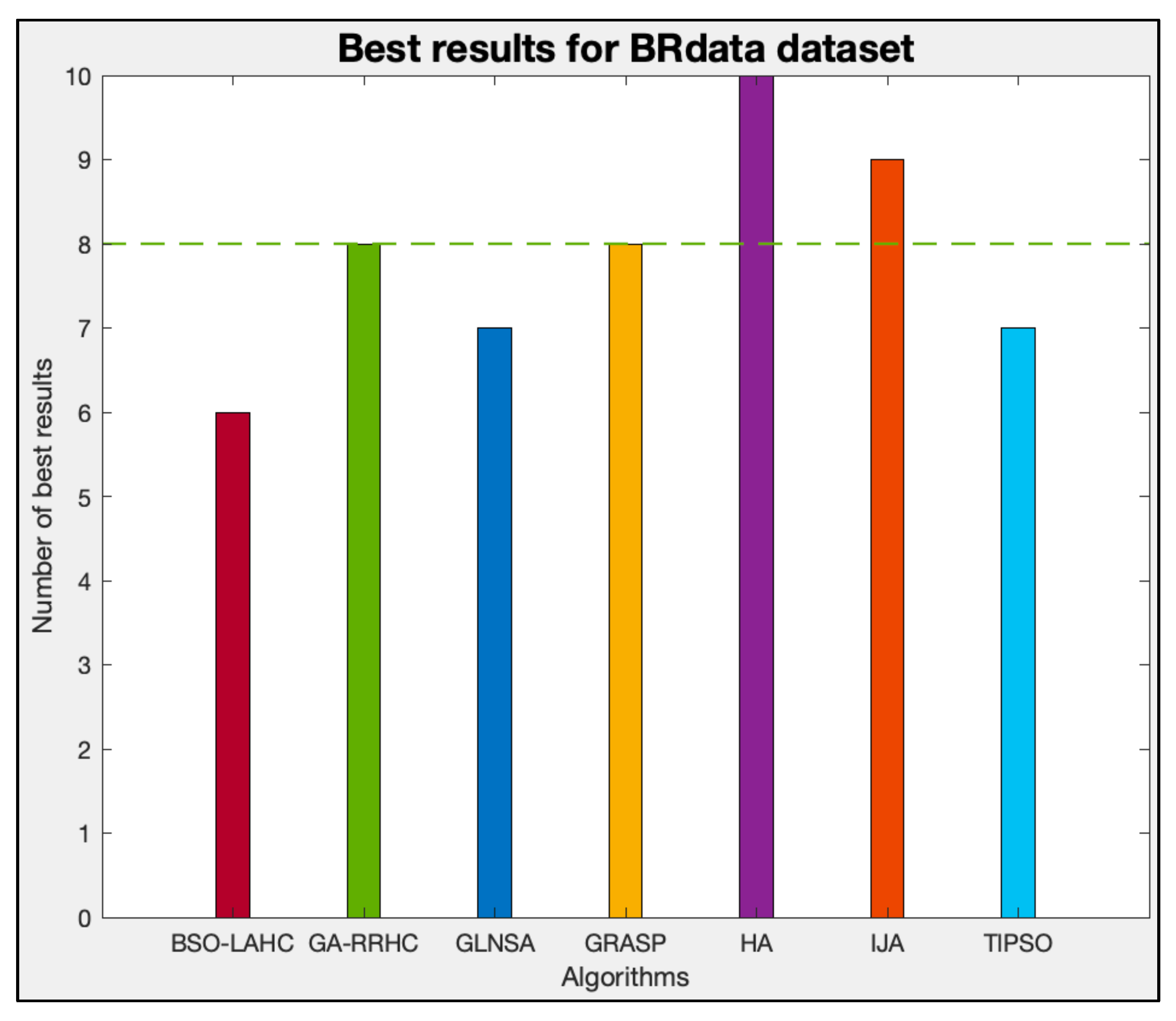
Table 5 provides the results of the GA-RRHC compared with the other methods for the BRdata dataset. In each case, the smallest obtained makespan is marked with *.
It can be seen in
Table 5 that the GA-RRHC calculates the least makespan in eight cases, behind the HA and IJA, and with the same optimal results as the GRASP.
Figure 14 shows the number of best results obtained for each algorithm in this dataset.
Table 6 shows the ranking of each method based on the average
, as well as the value
p of the non-parametric Friedman pairwise test, comparing the GA-RRHC with each of the other algorithms. The GA-RRHC secured the second place among the compared algorithms, obtaining a value of
with the BSO-LAHC and GRASP.
Figure 15 gives the signed difference between the average RPD of the GA-RRHC against the other methods in pairs. A negative difference means an inferior performance in contrast to the GA-RRHC.
This analysis indicates that the GA-RRHC is statistically competitive with the other four best algorithms for optimizing the BRdata dataset.
4.5. Rdata Dataset
This experiment takes the 43 instances of the Rdata dataset, with a flexibility rate
ranging from
to
. The results generated by the GA-RRHC are compared in
Table 7 with those obtained by the GLNSA, HA, and IJA, which are the methods that report results for this dataset.
Figure 16 depicts the number of best results obtained for each algorithm in this dataset, where the GA-RRHC calculated the 23 best values, behind the HA and IJA.
Table 8 sorts each algorithm with its average
and the comparative Friedman test. From the results, it can be noted that the GA-RRHC ranked third overall, as might be expected in instances with low flexibility. The statistical analysis shows no significant difference with the IJA.
Figure 17 shows the difference between the GA-RRHC and the other methods for the average RPD. A negative value means again an inferior performance compared to the GA-RRHC.
This experiment verifies that the GA-RRHC performs comparably to the IJA for problems with low flexibility and outperforms the GLNSA.
4.6. Vdata Dataset
This experiment takes the 43 instances of the Vdata dataset, all of which have a flexibility rate
. The results generated by the GA-RRHC have been compared again with those obtained by the GLNSA, HA, and IJA (
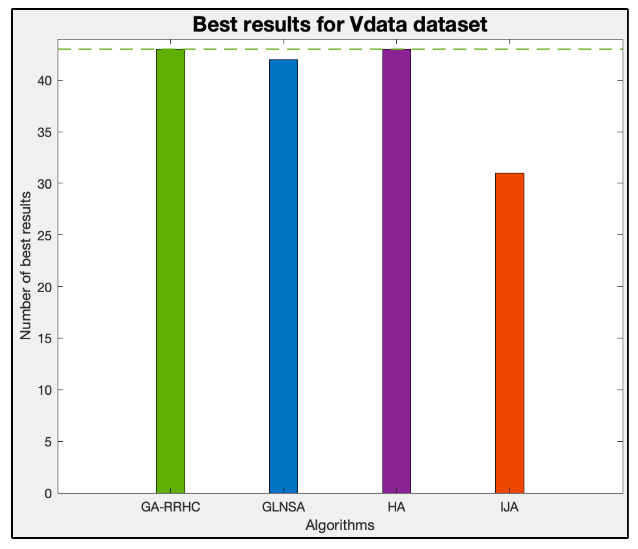
Table 9).
Figure 18 presents the number of best results obtained for each algorithm in this dataset, where the GA-RRHC calculated the 43 best values, the same as the HA and superior to the GLNSA and IJA.
Table 10 shows the ranking, the average
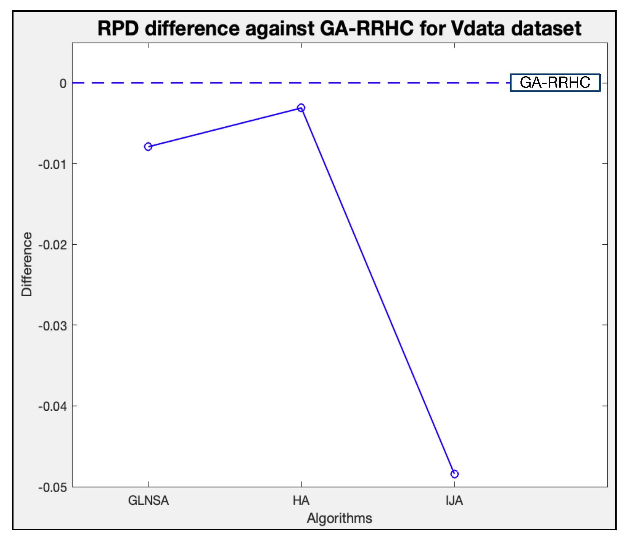
, and the non-parametric Friedman pairwise test values of each algorithm. The results show that the GA-RRHC obtained the first place concerning the RPD of the 43 problems, and the results indicate a significant difference with the IJA.
Figure 19 depicts the difference of the average RPD between the GA-RRHC and the other methods.
4.7. Generated Large Dataset
The previous experiments proved the correct performance of the GA-RRHC. However, the largest instance considers only 30 jobs, 10 machines, and 300 operations, which can be insufficient in real-world cases. Consequently, three randomly generated large instances were studied using the parameters established by [
17,
55]. These instances are named VL01, VL02, and VL03, considering from 50 to 80 jobs, from 20 to 50 machines, and from 704 to 2773 operations, with a flexibility rate
. Since these instances have not been used before in previous studies, we only apply the GLNSA for comparison, whose code is available in Github
https://github.com/juanseck/GLNSA-FJSP-2020 (accessed on 5 August 2022).
Table 11 shows that GA-RRHC performs much better than GLNSA, with enhanced performance for an increasing problem dimension.
Figure 20 presents three examples, one for each VL instance, of the optimization process achieved by the GA-RRHC. In the Gantt charts, it is remarkable how the idle times decrease from initial random solutions and the continuous convergence to calculate the minimum makespan.
These results corroborate that the GA-RRHC exhibits a performance comparable to recent algorithms recognized for their robustness in optimizing this type of problem, mainly for instances with high flexibility, and with competitive computational complexity.


 ,
, 


