1. Introduction
For children with different growth conditions, the differences in the growth process caused by the environment, genes, diet, etc., can usually be reflected by bone maturity, and then used to evaluate the development of children in cases such as endocrine disorders and pediatric syndromes. Therefore, assessing bone age is an important task in clinical application. In general, estimating the bone age of the non-dominant hand is the most commonly used method. Using the non-dominant hand to estimate bone age has several advantages. First, there are a lot of bones in palms. Second, the non-dominant hand is used less frequently and is less affected by external forces. Because most people’s non-dominant hand is the left hand, most estimates of bone age are based on the left hand. The assessment of bone age is mostly before and after puberty. For adults, due to the fusion of the growth plate, it is difficult to use the condition of the palm bones for assessment. Traditionally, there are two most commonly used methods for bone age assessment: the Greulich & Pyle Atlas (GP) method [
1] and the Tanner Whitehouse (TW) method [
2,
3]. In the GP method, the X-ray to be assessed for bone age is compared with the GP atlas to give bone age. This approach has several disadvantages. First of all, it takes a long time to assess bone age, and it also requires professional medical personnel to evaluate. Secondly, due to manual evaluation, there are human errors. In the TW method, 20 bones are scored separately, these scores are then combined to obtain a composite score, which is then mapped to a table to calculate bone age. Since bone age is determined by scoring, a possible problem is that an overly simplistic scoring method may lead to inaccurate estimates of bone age.
Since the above disadvantages lie in traditional bone age assessment methods, in the past, automatic bone age assessment systems have been proposed in many studies, while due to the development of deep learning technology, more and more systems for medical purposes are based on deep learning, including medical human–computer interfaces, medical diagnosis systems, medical data analysis, medical registration systems, etc. These various applications are increasingly inseparable from deep learning. For automatic bone age assessment systems, many studies also build their systems based on CNN. In these studies, the way of estimating bone age can be divided into two types. First, directly use CNNs to build a regression model for bone age [
4,
5], since this method is to fit all bone ages of palm bone X-ray by one CNN, in this case, the main problem is that if the estimation is wrong, it is easy to have great errors. Another way is to divide the palm bone X-ray into several stages according to the bone age [
6,
7]. At this time, the CNNs are dealing with the classification problem, however, the main problem of this method is that if the stages are divided too coarsely, the estimation of bone age will be not accurate enough. If the stages are divided too finely, the difference between the stages will be not obvious, which will cause it to be difficult to fit by CNNs and prone to overfitting. In order to avoid these problems, a compromise solution can be considered. First, the palm bone X-rays are divided into several rough stages, and for each stage an independent regression model is trained to estimate the bone age. Therefore, the accuracy of classification of the rough stages is very important. In this paper, we mainly deal with the problem of data imbalance in the classification at the coarse stage, and use the classification results to the CNN regression network to calculate bone age.
Although many existing bone age studies have trained a large number of palm bone X-ray databases [
8], which has led to good results on classification, however, due to differences in the growth process of children, due to differences in races, diets, and different growth environments, the development process of children varies in different regions. Therefore, it is necessary for each region to build its own bone age estimation system. For this reason, this paper is based on the palm bone X-ray films taken by children in Taiwan to build a system. In this case, we consider a problem: it will take a long time for X-ray data to accumulate to a sufficient number. Especially in toddler and post-puberty stages, there are few outpatient cases, so the data at these two stages will be greatly lacking. In the initial research stage of the bone age system, there will be a problem of very unbalanced data. For example, in this paper, in the three stages we use, the proportion of the database we collected in females is approximately 5:90:5, which is a very biased data distribution. In our follow-up experiments, we will find that when training directly with CNNs all the classification results are in the puberty stage.
This kind of X-ray data imbalance problem often occurs. For example, disease cases are usually much smaller than those without disease, or, as in the case of this paper, outpatient cases during toddler and post-puberty stages are very scarce, but these are a small number of cases, usually the system still must be able to distinguish them, so many existing studies are devoted to alleviating the problem of serious imbalances of X-ray data. The most commonly used methods are several: re-sampling the data by undersampling [
9,
10] or oversampling [
11,
12,
13,
14], using transfer learning [
15,
16,
17] to pre-train network parameters with other datasets with relatively sufficient data, and using the target task dataset to fine-tune the model. In addition, the loss function of its CNNs is improved [
18,
19,
20,
21]. The loss function is usually designed to compensate for a small number of classes during training.
The undersampling and oversampling methods each have their shortcomings. In oversampling, if the amount of data of certain classes is quite lacking, no matter how the data is augmented, the data generated by the augmentation is always generated from the original small amount of classes. Therefore, the features that can be learned in CNNs are still very limited. In undersampling, if we have to discard those samples from a large number of classes, it is a waste of these discarded data, especially in medical imaging where image collection is more difficult. By using the loss function to compensate for the small number of classes, the network is made to learn more towards the small number of classes to alleviate the data imbalance problem, but the network always learns all classes of datasets on the same network, which is still susceptible to a large number of classes. Therefore, in this paper, we use three (three-stages target in this paper) autoencoders [
22] and a CNN-based scoring network to alleviate the data imbalance problem, because in each stage each autoencoder is independent, they do not influence each other, so the small number stage will not be disturbed by the large number stage. In DIIBAA, the classification problem is turned into an image quality scoring problem. Its classification is mainly based on the features of image quality. However, the classification’s features are still precious information. Therefore, we also add a classifier for the bone age stage and integrate these two different results for the final judgment result. After the classification is completed, we use a CNN-based regression network to determine the bone age value.
In the subsequent section of this article, we first describe the dataset used in this article and detail the DIIBAA method proposed in this article in
Section 2, which includes two branches which use image quality features and classification features, respectively. And finally, we use the two to jointly determine the results of bone age stage prediction. After the stage prediction, we build the bone age regression models to evaluate the bone age. In
Section 3, we will show the experimental results and their comparisons. In
Section 4, we discuss the advantage and limitations of our method. In
Section 5, we give the conclusion of the DIIBAA method proposed in this article.
2. Materials and Methods
The datasets used in this paper are shown in
Table 1. These stages are based on [
23] (in fact, they have a total of 6 stages, we consider that the two stages are too similar, so the adjacent stages are merged). S
1 is the toddler stage, S
2 is the puberty stage, and S
3 is the post-puberty stage. The data set is from the Taoyuan Cheng Hsin General Hospital, and the labels are judged by two professional physicians. These two professional physicians refer to the clinical database in the hospital to give the bone age stage and the bone age value. In order to reduce human error, our bone age value is the average judgment of the two physicians. These data were collected by the hospital in 2018 to 2020. It can be found that in these three stages, regardless of gender, they are very unbalanced. As the follow-up experiments show, in this extremely unbalanced situation, when directly using CNN training, they are very unbalanced and both ends (S
1 and S
2) of stages have weak discernment.
In order to clearly illustrate the input data of this paper, we sample three pictures from each stage of the data in
Table 1, as shown in
Figure 1, from left to right are toddlers (S
1), puberty (S
2) and post-puberty (S
3) stages.
The DIIBAA consists of two branches, as shown in
Figure 2. Branch 1 consists of three autoencoders and a scoring network. This branch converts the classification problem into an image quality assessment problem, and because the high-quality images and low-quality images have been converted into 1:2, the problem of data imbalance in this branch can be greatly alleviated. In the second branch, the classification information is actually very valuable since the classification features are not used in the first branch, but the network trained directly using all the data is extremely imbalanced and relationships are almost indistinguishable for each stage. Therefore, in order to utilize classified information, we use mixup data augmentation [
24] on branch 2 to alleviate the problem of data imbalance and make the network slightly more distinguishable. For the samples that are ambiguous in the first branch, we use branch 2 to judge them, and finally, give a CNN-based regression network to the three bone age stages, respectively, and use it to give the bone age values. In short, we first use branch 1 to predict, then check its results. If the check is passed, the bone age prediction stage is the result of branch 1, otherwise, branch 2 is used as the result of the bone age prediction stage.
2.1. Autoencoder-Based Scoring Classification System
In branch 1, we use three autoencoders to represent three stages (S
1~3 in
Table 1). In each autoencoder, the input and output image sizes are 224 × 224. During the encoding process, we have a total of three convolutional layers, their kernel size are all 3 × 3, and the number of channels from the first layer to the third layer are 512, 256, and 128, respectively. After each convolutional layer, a pooling layer is followed, and in each pooling is the reduced feature map which is 1/2 times that of the previous layer. In the decoder part, the convolution kernels from shallow to deep layers are 128, 256, and 512, respectively. The rest of the convolution kernel parameters are the same as those of the encoder. After convolution, they are all upsampled to double the size of the previous layer, and finally, a single-channel 1 × 1 convolution layer will be connected. The output of this layer represents the reconstructed image. The sigmoid function is used in this layer for nonlinear transformation, and the rest are all ReLU. The architecture of a CNN-based autoencoder is as shown
Figure 3. In the scoring network, we use DesnseNet169 [
25], we use it for the regression of score, so the output layer activation function is sigmoid. In the following, we will divide the training and testing phases to illustrate the branch 1 part in this paper.
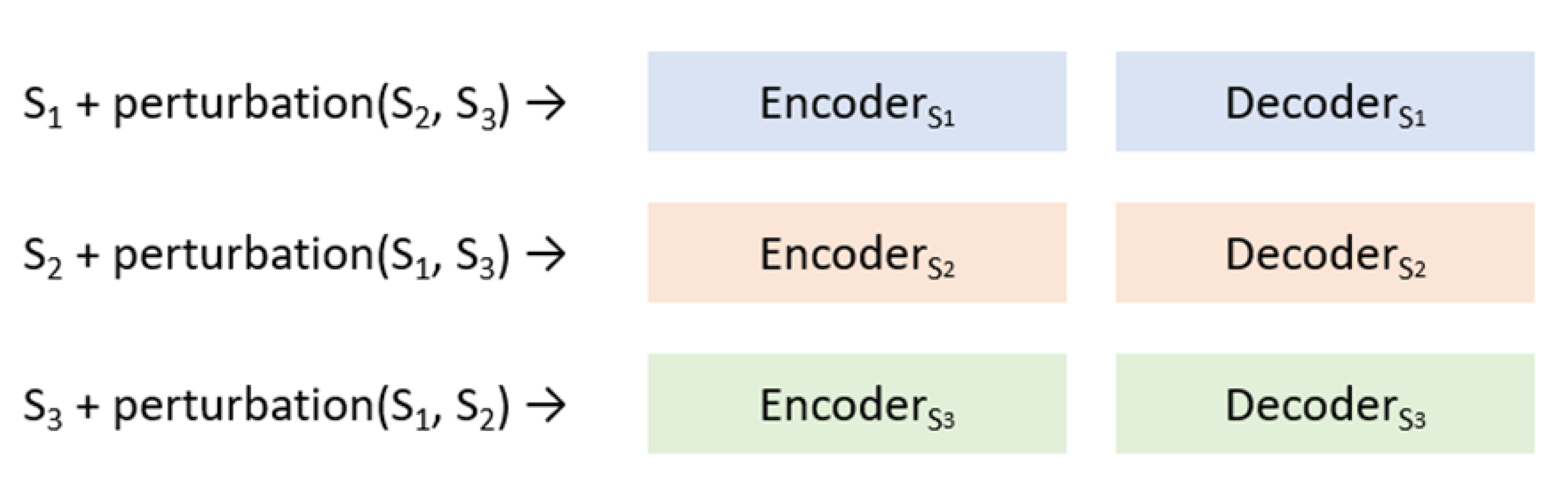
In the phase of training, we first train three autoencoders. As shown in
Figure 4, we use the corresponding autoencoders for training. For example, in the blue branch, we only use the data in the S
1 stage for training. In the orange branch, only the training of the data in the S
2 stage is used. During the training process, we add the perturbed data of the other stages to weaken the reconstruction ability of the images that are not of our own stage. The input of the perturbed data pair is the original image, and the output (that is labeled) is the result of perturbing the original image. In this paper, the perturbation in the branch is Gaussian noise [
26]. Density in Gaussian noise simulation are added to the image in a random way. Its SNR value is about 6.989 to 10, and the SNR value is calculated as: SNR = 10 × log10(signal/noise). The number of perturbed degraded images in this paper is 5% of the images of this stage.
After the training of the three autoencoders is completed, we will then use the reconstruction results of these three autoencoders to generate data for the scoring network as training data. The training data we generate will eventually generate two classes, T and F. T is the result after the training image is reconstructed by the autoencoder of its own corresponding stage. For example, the image of the S
1 stage is reconstructed by autoencoders1, and F is the result of the training image reconstructed by the autoencoder of its own non-corresponding stage. For example, the image of the S
1 stage is reconstructed by autoencoders
2 or autoencoders
3, such as (1) and (2):
Among them, Decoder_S
1 and Encoder_S
1 are the encoding and decoding functions (CNNs) of stage S
1, respectively, and S
1, S
2 and S
3 are the training X-ray data. After taking the data of the two sets of T and F, we set T as 1.0 points, F as 0.0 points, using such a configuration to train the scoring network, here we can see that the ratio of T to F is 1:2 (each image will generate 1 T and 2 F), which is a considerable alleviate for the original extremely imbalanced data (
Table 1).
In the test, when an image X is an unknown stage, we first input X to three different autoencoders, they will generate X
S1r, X
S2r and X
S3r, three images, as shown in
Figure 5.
Then, input X
S1r, X
S2r and X
S3r into the scoring network, respectively, and each will receive a score of either X
S1r, X
S2r or X
S3r, as shown in
Figure 6:
Finally, X is predicted to be the stage corresponding to the autoencoder network corresponding to the highest score of X
S1r, X
S2r and X
S3r, as shown in Equation (3):
In branch 1, our principle is that if the image is input into the non-corresponding autoencoders, these autoencoders should not be able to reconstruct it well, conversely, if the X-ray image is input to the corresponding autoencoder there should be excellent reconstructed image quality. Therefore, in the scoring network, we can say that it predicts the image quality to give the input image score. Therefore, if the image has a better reconstruction effect in a certain autoencoder, the image should be the corresponding class for this autoencoder.
2.2. Use Mixup Augmentation to Train CNN Network
Since the above-mentioned way of independent autoencoders does not mainly take into account the fact that the images are actually distinguishable features, in order to keep these features from being wasted, we use a CNN that also builds classification purposes to make DIIBAA’s system also take into account classification features. Since CNN is directly used to classify these extremely unbalanced data, they have almost no classification ability (experimental description in the next chapter). Therefore, we use the mixup augmentation [
24] method to augment the data of S
1 and S
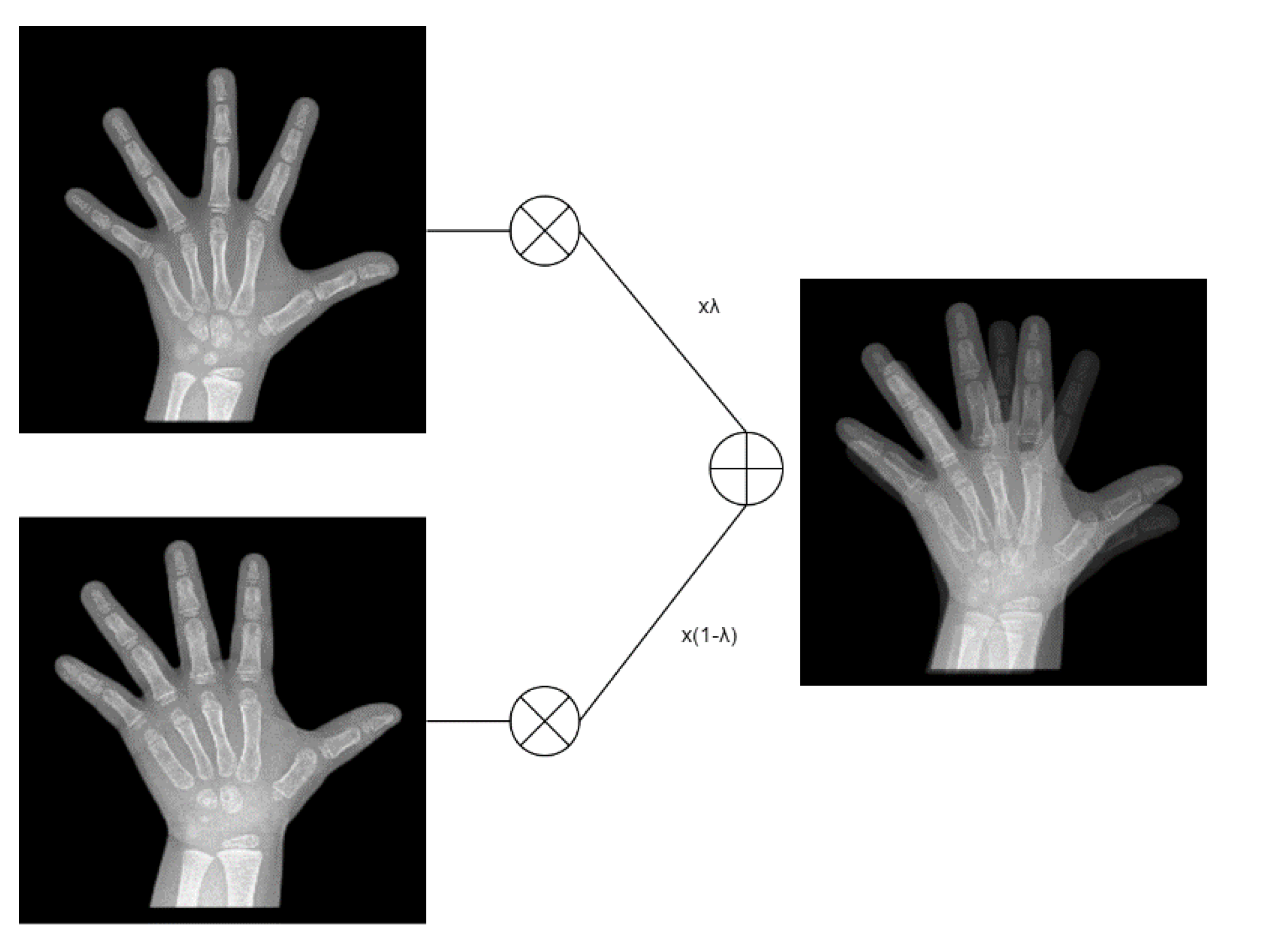
3. The mixup augmentation is as follows (4): The formula:
In the above equation,
represents the synthesized image, and
is a value of 0–1. Here we generate λ in a random way,
and
are two randomly selected images, respectively, and here we use Formula (4) for the X-ray films of the S
1 and S
3 stages to generate synthetic images until the number of images in S
1 and S
3 is equal to the number of images in S
2.
Figure 7 is a mixup operation, using (4) to superimpose two images at the same bone age stage with the random
.
With this data we train a CNN network, called, CNN_mixup, which is an improvment compared to the indistinguishable (without mixup) augmentation, as shown in
Table 2 and
Table 3 (female and male, respectively):
When using mixup augmentation, compared to 0% at both ends before no augmentation, with mixup augmentation the two end stages in female are increased from 0%, 0% to 41.67%, 30.77%, and male from 0.00% and 33.33% to 41.67%, 66.67%, respectively. Such a result shows that CNN_mixup has some discrimination ability.
2.3. Integration 2model
Next, we must integrate the results of the two branches. First, we use the results of the scoring network. If the difference between their top two scores > th_score, then since the network with the highest score is significantly better reconstructed than the other two, this indicates that it has a fairly high chance for this stage, so in this case, we take the final classification result as the result of the scoring network, otherwise the predicted result using CNN_mixup is the final output result. The details are shown in Algorithm 1:
| Algorithm 1. Integration 2 model |
| Input: Encoder_S1, Encoder_S2, Encoder_S3, Scoring_CNN, CNN_mixup, image_x, th_ score |
| Sc1(image_x) = Scoring_CNN(Encoder_S1(image_x)) |
| Sc2(image_x) = Scoring_CNN(Encoder_S2(image_x)) |
| Sc3(image_x) = Scoring_CNN(Encoder_S3(image_x)) |
| hs = highest score(Sc1(image_x), Sc2(image_x), Sc3(image_x)) |
| shs = second highest score(Sc1(image_x), Sc2(image_x), Sc3(image_x)) |
| If hs – shs > th_score |
| Result = hs |
| Else |
| Result = result of CNN_mixup |
| Return Result |
Next, we find a suitable th_score, we use Algorithm 2 to find this threshold. On the validation set, at an interval of 0.1, find the th_score with the highest accuracy for the overall validation.
| Algorithm 2. Finding th_score |
| Input: Algorithm 1, validation data |
| Highest accuracy = 0.0 |
| For th from 0.05 to 0.5 |
| Accuracy = Algorithm 1(validation data, th) |
| If Accuracy > Highest accurazy |
| th_score = th |
| Return th_score |
In this step, we use a CNN regression model to assessment bone age values. In the dataset of
Table 1, bone age values are in years and include decimal points (example: 6.5 years means 6 years and 6 months). We built three independent regression models for each of the three bone maturation stages (S
1~3), and before training the CNN regression model, we normalized the value of bone age to range from 0 to 1. We use the Equation (5) for normalization.
In (4),
represents the normalized bone age value, and
represents the original bone age value. After regressing the results given by the network, we use Equation (6) to calculate the true bone age value.
In (5), BA represents the final predicted bone age, the base is the minimum bone age value in the connection, as shown in the
Table 4, the scale is the bone age range at this stage, maximun BA–minimum BA.
3. Results
In our experiments, we use DenseNet169 as the backbone of CNNs, and the baseline represents the original DenseNet169 architecture, and directly classify the three stages in
Table 1. The branch 1 column represents the results using three independent autoencoders and scoring networks. The branch 2 column uses the exact same architecture as the baseline. The difference is that the training data is augmented by mixup. DIIBAA is the final staged result of the system in this paper. The th_score calculated by Algorithm 2 is 0.45 and 0.6 for female and male, respectively, according to the validation set results. These results are shown in
Table 5 and
Table 6, which represent boys and girls, respectively. The following accuracies are all test set accuracies, 80% are training and validation sets, and 20% are test sets. The amount of data is shown in
Table 1 above.
As these two tables show, the baseline, S1 and S3 have almost no recognition ability, and even in females, all inputs are predicted as S2. Although the performance of the autoencoder drops in S2, it has at least some discriminative ability in the two minority stages S1 and S3, the drop in the S2 stage does not imply that the baseline has a better ability to identify S2, for example, for male, it just predicts all inputs as S2. In branch 1, although its performance is worse than that of autoencoder at both ends, it has less degradation to S2, which allows us to use the results of branch 2 to improve the insufficiency of branch 1 for S2 accuracy.
Next, in
Table 7 and
Table 8, we list the results for all th_scores. It can be found that the th_score needs to be high enough to have good performance. This is because when the th_score is too low (because branch 1 uses the image quality score as the classification basis) the image quality is not much different, and the result of branch 1 is easily susceptible to errors. Therefore, the th_score is used to adjust the output result, so that the classification result of branch 1 is used when th_score is appropriately high, otherwise the result of branch 2 is used as the finally result.
Here, we must compare with other methods for data imbalance problem alleviation. We adopt three methods commonly used to alleviate the data imbalance on CNN on our data set. We employ these methods on the task of bone age stage identification task and use their staged identification results to input into the corresponding bone age estimation regression network. We compare the application research of these three methods in the medical images. The three methods are: oversampling method, ref. [
14] using DCGAN [
27] to perform data augmentation for the minority classes, ref. [
21] using focal loss [
28] to deal with data imbalance problem, ref. [
17] is based on transfer learning (ImageNet as the source domain dataset) and data augmentation to deal with the imbalance problem. In the first two methods, we still use densenet169 as the backbone network. In [
17], since they pointed out that Xception is the most superior in their method, we use Xception as the backbone network in the method of [
17].
Table 9 and
Table 10 are the comparison of accuracy and MAE, respectively.
As shown in
Table 9 and
Table 10, DIIBAA outperforms the other three methods on the problem of this article. We explain these reasons for each method separately. There are two main problems with the DCGAN-based method. First, if the DCGAN cannot be well trained, their help for data augmentation is limited. In addition, as we mentioned earlier, this kind of oversampling method usually just augments the existing data, they are helpful in the expansion of the decision boundary, but since the amount of data in our two stages is too scarce, this method will have ineffective results. For focal loss, it strengthens training on hard samples (equivalent to the minority stages in this article), and minority stages are actually too scarce, so the focal loss is still not enough for training in hard samples. Therefore, its method has a considerable improvement over the baseline network, but still not accurate enough. In the transfer learning-based method, since this method does not directly design data imbalance, it may be more helpful for slightly imbalanced data, but it performs poorly for the more difficult cases of this article.
In the comparison of MAE, due to the stage prediction error, the error caused by it is even greater, and DIIBAA is still better than the above three methods because of its error rate. Of course, the MAE of DIIBAA has better results.
Finally, we use experiments to explain why we need to classify the mature stages of bone age first, instead of directly using a regression CNN for all stages. We calculate the MAE of the two to compare, and the results are shown in last column of
Table 10.
It can be found that when the bone age is directly regressed without distinguishing stages, the error of their MAE is very large, compared with the first stage. This is because when all stages are mixed training, the range between them is larger and the variation is larger. This makes CNN regression harder to fit. When the stages are separated, each independent network fit is less problematic and therefore more likely to have accurate results.
4. Discussion
Although our results have been greatly improved compared to the case where the baseline has almost no discriminative ability, there is still the possibility of further improvement in the future. In the branch 1 part, there still can be improvement in the S1 and S3 stages. In future, we can try to enhance it in the following ways, such as adding richer perturbation of the autoencoder, and the improvement of the loss function of the scoring network, etc. I believe that under the framework of this paper, there is still a certain potential to further improve this extremely imbalanced data. In the part of mixup augmentation, this is a way of oversampling. Maybe we can think about how to make the data generated in the process of oversampling more diverse, so that the decision boundary of a small number of classes can be more practically expanded, and then make the branch 2 network more distinguishable. If the two branches can be further improved, I believe that the DIIBAA system can give more reliable classification results.
Additionally, this paper uses autoencoders and scoring networks to build a system to alleviate data imbalanced problem. We also suggest that this method is quite suitable to alleviate the data imbalance problem encountered by other medical images, but there is a problem to consider, we convert the data ratio to 1:2. However, if the dataset has many classes, such as a dataset with 100 classes, then the ratio of DIIBAA will become 1:99 in the training of the scoring network. At this time, we can consider the operation of undersampling the F category, which is different from directly undersampling a large number of categories, because in 99% of the data in F, each data actually has another 99 of the same origin. For the data generated by the graph, each original graph has a high probability to exist in F, and must exist in T, so data will not be wasted.
Finally, with the migration of the ages, the living conditions of human beings will inevitably change, and with the changes in eating habits, living habits, etc., the developmental process of children will inevitably change, and the method in this article is built using a changeless data set (2018 to 2020), in the face of future changes, the system must be able to update the model with the times, such as adding online learning methods.
5. Conclusions
Automatic BAA is an important task for pediatrics, and in order to accurately assess bone age, in the experiment, we show that assessment of bone age in divided stages is a better way. Therefore, the stage is independently given to a regression network before we must first perform stage prediction on the unknown X-ray films, and in order to train the stage discriminant classifier, we meet a serious data imbalance problem. If we directly use them for CNN training, the CNN has almost no discriminative ability. It is just that almost all samples are predicted as a large number of stages. Therefore, this paper mainly converts the classification problem into an image quality assessment problem, because the autoencoders in these stages are independent and do not interfere with each other, which naturally avoids data imbalance problems. In addition, considering that the classification features between these X-ray films are also valuable information, in order to effectively utilize them, we use mixup data augmentation to make branch 2 in DAIIBA system have some classification ability, and finally we use th_score to leverage the advantages of both of them. Finally, we also show that the correct prediction of bone age stage is helpful for the prediction of bone age value.


