Improving Adversarial Robustness of CNNs via Maximum Margin

Abstract

In recent years, adversarial examples have aroused widespread research interest and raised concerns about the safety of CNNs. We study adversarial machine learning inspired by a support vector machine (SVM), where the decision boundary with maximum margin is only determined by examples close to it. From the perspective of margin, the adversarial examples are the clean examples perturbed in the margin direction and adversarial training (AT) is equivalent to a data augmentation method that moves the input toward the decision boundary, the purpose also being to increase the margin. So we propose adversarial training with supported vector machine (AT-SVM) to improve the standard AT by inserting an SVM auxiliary classifier to learn a larger margin. In addition, we select examples close to the decision boundary through the SVM auxiliary classifier and train only on these more important examples. We prove that the SVM auxiliary classifier can constrain the high-layer feature map of the original network to make its margin larger, thereby improving the inter-class separability and intra-class compactness of the network. Experiments indicate that our proposed method can effectively improve the robustness against adversarial examples.

1. Introduction

Convolutional neural networks (CNNs) have been widely used in various domains, especially in computer vision. CNNs have satisfying learning capabilities as they can extract image features of different scales by multiple convolutional layers. However, various CNN architectures are vulnerable. The models will predict wrong results with small perturbations adding to the inputs that humans cannot recognize. In other words, adversarial examples [1,2,3], which are similar to clean examples, will mislead the CNN to output incorrect results. Moreover, adversarial examples can transfer across different CNN models [4,5]. These phenomena indicate that the CNN learns some simple patterns to accomplish tasks exactly on specified data but does not recognize more robust advanced features like the human brain. So the CNN is not safe for medical care [6], autonomous driving [7], and other fields.

The potential serious harm of adversarial examples has drawn the attention of the scientific research community, forming a new field called adversarial machine learning. There are two main types of defense methods against adversarial examples, i.e., certified methods and empirical methods. Certified methods [8,9] can obtain provable robustness, but the provable robustness is low and most of them only aim at the attack with disturbance of $l_2$ norm. Empirical methods account for the majority of defense methods, including stochastic activation pruning (SAP) [10], distillation defense [11], asymmetrical adversarial training [12], ME-net [13], etc. However, the robustness of empirical methods is not reliable, and it may be broken by stronger attacks [14,15].

Adversarial training (AT) [16] is one of the most successful empirical defense methods at present which is a data augmentation technique for training models on both natural and adversarial examples. Although AT is an empirical method, it has been proved to be highly robust even under adaptive attack [14]. AT effectively robustifies CNN but has two challenges: lower clean accuracy [17] and the overfitting problem [18,19]. To address these challenges, many variants of AT have been proposed, such as TRADES [20], customized adversarial training (CAT) [21], dynamic adversarial training (DAT) [22], and geometry-aware instance-reweighted adversarial training (GAIRAT) [23]. However, these two problems are still unsolved very well. So this paper is devoted to them by considering the maximum margin.

The key insight is that the purpose of adversarial machine learning, i.e., the maximizing margin is very similar to that of SVM. Theoretically, the margin of the classifier in the input space is positively correlated with its robustness. However, for multi-layer neural networks, the margin on the input space is difficult to be calculated and constrained. AT can indirectly increase the margin of the classifier in the input space because the adversarial examples are obtained by moving clean examples toward the decision boundary. We find that ordinary training methods such as using cross-entropy loss cannot effectively increase the margin. So we propose adversarial training with supported vector machine (AT-SVM) that increases the margin by SVM. Specifically, we insert an SVM auxiliary classifier before the last layer in the network, which can maximize the margin on this feature space. The SVM is a better classifier for high-level feature space, so we use it to identify more confusing points which will be trained on the original network. With continuous learning, the boundary of the original network will gradually approach the boundary of the SVM. At the same time, in order to ensure that the margin on the feature space is consistent with the margin on the input space, we constrain the distance between the clean example and the corresponding adversarial example in the margin direction of this feature space. Experiments indicate that our proposed method can effectively improve the robustness against adversarial examples.

2. Related Work

In this section, we briefly review the adversarial training and defense methods based on it.

2.1. Adversarial Attacks

With the proposal of adversarial examples, the earliest method used to generate adversarial examples is the fast gradient sign method (FGSM) [1]. FGSM generates adversarial examples with a single normalized gradient step. Since then, a number of gradient-based and multi-step iterative attacks have been proposed such as projected gradient descent (PGD) [16], C&W attack [24], and DeepFool [25]. We review the PGD attack which is the most popular and widely used attack.

PGD aims to find an adversarial example $\widehat{\mathit{x}}$ for an input $\mathit{x}$ that satisfies a given boundary $\left|\right|\widehat{\mathit{x}}-\mathit{x}{\left|\right|}_p<ϵ$. Let B denotes the $l_p$-ball of radius $ϵ$ centered at x. The attack initializes the adversarial example with a random point $x_0\in \mathit{B}$, and iteratively updates it with the gradient, as shown in Equation (1).

$$\begin{array}{cc}\hfill & {\mathit{x}}_{i+1}={Proj}_{\mathit{B}}\left(x_i+\alpha ·g\right)\hfill \\ \hfill & \mathrm{s}.\mathrm{t}.g=\underset{{\parallel v\parallel }_p\le 1}{argmax}{v}^{\top }{\nabla }_{{\mathit{x}}_i}L\left(f\left({\mathit{x}}_i\right),y\right)\hfill \end{array}$$

(1)

where $L\left(.,.\right)$ is a suitable loss-function (e.g., cross-entropy), f is the objective model, $\alpha$ is a step size, ${Proj}_B$ projects an input onto the $l_p$-ball B, and g is the direction of gradient that loss ascents fastest for a given $l_p$-norm. For the $l_{\infty }$-norm, ${Proj}_B$ is a clipping operator and $g=sign\left({\nabla }_{x_i}L\left(x_i,y\right)\right)$.

2.2. AT-Based Defense Methods

For a CNN model with parameters $\theta$, the goal of adversarial defense is to solve the following min-max optimization problem, as shown in Equation (2)

$$\underset{\theta }{min}{\mathbb{E}}_{(x,y)\sim D}\underset{\widehat{\mathit{x}}\in {\mathbb{S}}_0\left(\mathit{x}\right)}{max}\mathcal{L}\left(h_{\theta }\left(\widehat{\mathit{x}}\right),y\right)$$

(2)

where the inner maximization is intractable, so adversarial training replaces it with a lower bound which is obtained by an adversarial attack. The standard adversarial training (SAT) [16] maximized the inner loss using PGD attack and found it performs well against other adversarial attacks.

Several improvements for standard adversarial training have been proposed. Curriculum adversarial training [26] trains a model from weak attack to strong attack. Dynamic adversarial training (DAT) [22] proposes a dynamic training strategy to increase the convergence quality of the generated adversarial examples gradually. TRADES [20] traded adversarial robustness for accuracy. Misclassification aware adversarial training (MART) [27] explicitly differentiates the misclassified and correctly classified examples during the training. Friendly adversarial training (FAT) [28] searches for the least adversarial data (i.e., friendly adversarial data) by minimizing the loss that makes results confidently misclassified rather than employing the most adversarial data to maximize the loss. Customized adversarial training [21] proposes auto-tuning perturbation and adaptive label smoothing for adversarial training. Gowal et al. [29] improved the state-of-the-art robustness by largening the model’s Swish/SiLU activations and model weight averaging. Geometry-aware instance-reweighted adversarial training (GAIRAT) [23] regards iterations needed for an attack to misclassify an example as its importance and then uses it to reweight all training examples.

2.3. AT-Used Defense Methods

In addition to the improvements of AT, there are many defense methods requiring the assistance of AT to implement specific functions or achieve higher robustness.

Mustafa et al. [30] learned centers in hidden feature space to separate higher-order representations of different classes. Taghanaki et al. [31] proposed a defense strategy based on kernel function, which increases robustness through learnable Mahalanobis distance. Channel-wise activation suppressing (CAS) [32] suppressed redundant activation from being activated by adversarial perturbations. Ref. [33] used spatial attention to realize adversarial robustness. Channel-wise importance-based feature selection (CIFS) [34] built a probe network to get the importance mask for each channel. Feature denoising [35] uses non-local mean filtering, mean filtering, median filtering, and bilateral filtering to perform feature denoising for improving the robustness of countermeasures.

These methods have changed the network structure and used it as the main contribution, and need to be combined with adversarial training. Although they provide a theoretical basis for changing the network structure, it is difficult to get effective improvement if the adversarial training is not added at the same time in the experiment (even if there is, it is probably due to gradient masking).

3. Proposed Method

In this section, we firstly introduce the motivation and basic theories of our proposed method. Then we consult its learning objective as well as its algorithmic implementation. Lastly, we compare our method with other existing defense methods.

3.1. Motivation

On the one hand, according to a common empirical result from researchers of adversarial defense [16,23], a larger model capacity is needed for adversarial examples. Therefore, in the case of insufficient model capacity, it is unwise to treat all examples equally. Training more important examples is helpful to make better use of the model capacity. On the other hand, intuitively, the examples close to the classification boundary are more vulnerable to adversarial attacks and are more important for the classification boundary. This widely accepted assumption can be proved empirically. 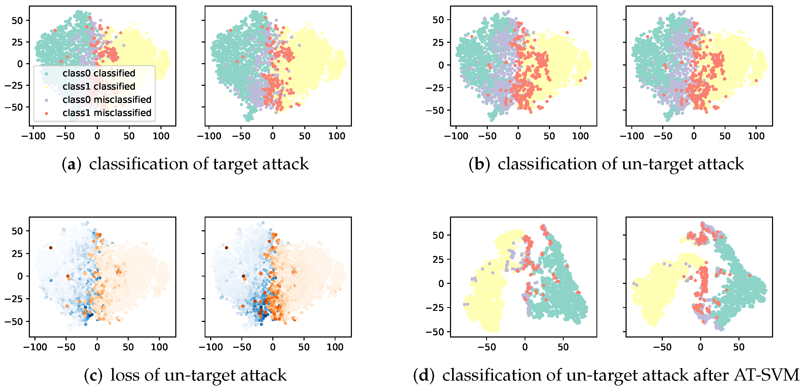Figure 1 shows the distribution of the feature map before the last layer of the two randomly selected classes in the CIFAR-10 dataset. It can be seen that the features of the misclassified examples are concentrated near the boundary no matter whether it is adversarial examples using targeted or untargeted attack.

According to the idea of SVM [36], to obtain a linear binary classifier that maximizes the margin between two classes, only the examples closest to the decision boundary, i.e., the support vectors, are needed. For a CNN network, although it is not a linear classifier, the last layer is always a fully connected (FC) layer that is linear. So the examples can be transformed into linearly separable high-order feature space after passing the front layers. According to these high-order features, we can find out which examples are support vectors that are close to the boundary. Training models on these examples can improve the efficiency of adversarial training.

For linear classification tasks, SVM can learn the classifier with the largest margin. We extend the SVM and add an SVM auxiliary layer into the CNNs when training so that the features extracted by the CNNs have a larger margin, hence improving the adversarial robustness of the CNN.

3.2. Theories

3.2.1. Linear Binary-Classification Task

For a binary linearly separable classification problem, there exist many hyperplanes that might classify the data. SVM is designed to compute the classification hyperplane which represents the largest separation, or margin, between two classes. The max-margin hyperplane is also known as the optimal classification hyperplane.

The main idea of finding the optimal classification hyperplane is to maximize the distance between different classes. Because of the possible inseparable points in data, slack variable $\zeta$ and penalty coefficient C are generally added. So the essence is to solve the following optimization problems, as shown in Equation (3)    

$$\begin{array}{cc}\hfill & min\frac{1}{2}{\parallel \mathit{\omega }\parallel }_2^2+C\sum _{i=1}^m{\zeta }_i\hfill \\ \hfill & s.t.y^{\left(i\right)}\left({\mathit{\omega }}^T{\mathit{x}}^{\left(i\right)}+b\right)\ge 1-{\zeta }_i\hfill \\ \hfill & {\zeta }_i\ge 0,i=1,2,\dots ,m.\hfill \end{array}$$

(3)

where $y^{\left(i\right)}=\pm 1$ indicate that ${\mathit{x}}^{\left(i\right)}$ is a positive or negative example.

These constraints of the optimization problem in Equation (3) can be solved by mathematical methods such as the sequential minimal optimization (SMO) [37] algorithm. However, in order to replace the original linear FC layer in the training of CNN, this formula cannot be directly used as a new loss function, as there are inequality constraints. So the following content will deform this optimization problem.

The constraints are equivalent to Equation (4).

$${\zeta }_i\ge max\left(0,1-y^{\left(i\right)}\left({\mathit{\omega }}^T{\mathit{x}}^{\left(i\right)}+b\right)\right)$$

(4)

The inequality constraint in Equation (4) shows the lower bound of ${\zeta }_i$. When solving the minimization problem outside, we approximately replace ${\zeta }_i$ with the lower bound of it. Let $C^{\prime }=1/2C$. Equation (3) can be written as Equation (5).

$$min\sum _{i=1}^{m}max\left(0,1-y^{\left(i\right)}\left({\mathit{\omega }}^T{\mathit{x}}^{\left(i\right)}+b\right)\right)+C^{\prime }{\parallel \mathit{\omega }\parallel }_2^2$$

(5)

Since there is no inequality constraint, the new formula can be directly used as the loss function. Notice that ${\sum }_{i=1}^{m}max\left(0,1-y^{\left(i\right)}\left({\mathit{\omega }}^T{\mathit{x}}^{\left(i\right)}+b\right)\right)$ is the hinge loss function. The other item $C^{\prime }{\parallel \mathit{\omega }\parallel }^2$ can be regarded as a regularization term added to improve the generalization performance of the model.

3.2.2. Linear Multi-Classification Task

For a multi-class classifier, the predicted label is chosen by the maximal logit attained over all classes:

$$\widehat{y}=arg\underset{k}{max}{f}_k\left(\mathit{x}\right)$$

where $f_k\left(\mathit{x}\right)$ is the output of $f\left(\mathit{x}\right)$ corresponds to the kth class. In linear case, $f_k\left(\mathit{x}\right)={\mathit{\omega }}_k^T\mathit{x}+b_k$.

For any two classes $(p,q)$, the decision boundary between them is called $l_{p,q}$.

$$\begin{array}{cc}\hfill l_{p,q}& =\left\{\mathit{x}\mid {\mathit{\omega }}_p^T\mathit{x}+b_p={\mathit{\omega }}_q^T\mathit{x}+b_q\right\}\hfill \\ & =\left\{\mathit{x}\mid \left({\mathit{\omega }}_p^T-{\mathit{\omega }}_q^T\right)\mathit{x}+b_p-b_q=0\right\}\hfill \end{array}$$

(6)

The geometric distance of a point $\mathit{x}$ from $l_{p,q}$ is:

$$d_{p,q}\left(\mathit{x}\right)=\frac{\left({\mathit{\omega }}_p^T-{\mathit{\omega }}_q^T\right)\mathit{x}+b_p-b_q}{{∥\left({\mathit{\omega }}_p^T-{\mathit{\omega }}_q^T\right)∥}_2}$$

(7)

Some margin-based methods only consider the margin between the ground truth class and the most easily misclassified class, i.e., setting $p=y,q=arg{max}_{i\ne y}{f}_i\left(\mathit{x}\right)$. Instead, our method considers all margins between each class and the other classes. In other words, we regard a multi-classification task as a multiply binary classification task. Equation (5) can be generalized to the following optimization problem in Equation (8).

$$\begin{array}{cc}\hfill min\sum _{i=1}^m\sum _{j=1}^{n}max& \left(0,1-y_j^{\left(i\right)}\left({\mathit{\omega }}_j^T{\mathit{x}}^{\left(i\right)}+b_j^T\right)\right)+C^{\prime }{\parallel {\mathit{\omega }}_j\parallel }_2^2\hfill \end{array}$$

(8)

where n is the class number, $y_j^{\left(i\right)}=\pm 1$ indicate ${\mathit{x}}^{\left(i\right)}$ is/not belong to class j.

3.2.3. General Classification Task

For a nonlinear classifier, the approximation scheme from Elsayed et al. [38] can be adopted to capture the distance of a point to the decision boundary which is a first-order Taylor approximation to the true distance. Equation (8) can be extended to:

$$d_{p,q}\left(\mathit{x}\right)=\frac{f_p\left(\mathit{x}\right)-f_q\left(\mathit{x}\right)}{{∥{\nabla }_{\mathit{x}}{f}_p\left(\mathit{x}\right)-{\nabla }_{\mathit{x}}{f}_q\left(\mathit{x}\right)∥}_2}$$

(9)

Using this approximation, we can calculate margins on all layers, just replace the input $\mathit{x}$ in the above formula with intermediate features ${\mathit{x}}^l$ on different layers. The training data $\mathit{x}$ induces a distribution of distances at each layer l which, following earlier naming convention [39,40], we refer to as margin distribution (at layer l).

Intuitively, constraining the margin distribution of the total network to be large enough can lead to a robust model. However, this approximation will lose accuracy fast as inputs move away from the decision boundary. Moreover, it is difficult to learn a model with large margin distribution. So that our proposed method only constrains the margin distribution on the last FC layer, just solve the optimization problem in Equation (8). At the same time, use $l_{margin}$ introduced later to limit the deviation between the margin distribution on the last FC layer and the margin distribution of the total network.

3.3. AT-SVM

In this section, we introduce our supported vector machine adversarial training (AT-SVM) method, which dynamically learns an SVM auxiliary classifier and restricts the decision boundary of the original network to achieve a large margin.

3.3.1. Overview

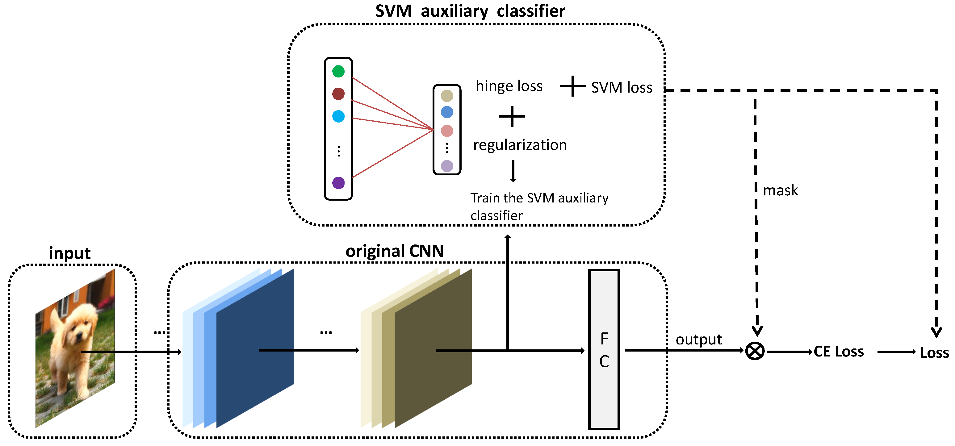
As Figure 2 shows, our method is mainly inserting an auxiliary SVM classifier in the penultimate layer of the network, which is parallel to the last layer. The SVM layer contains as many neurons as the number of classes and is purposed to obtain the maximum margin decision boundary in this feature space. The SVM auxiliary classifier treats the front layer of the original network as a feature extractor and uses a separate optimizer for training. In each epoch of training, the SVM auxiliary classifier and the original network are trained successively, and a mask on which examples will be trained is produced by the SVM auxiliary classifier. The SVM auxiliary classifier is discarded during inference. The specific implementation will be introduced in the algorithm.

In CNNs, the last FC layer is linear, so we regard the front layers as a feature extractor. Using $\varphi$ to denote the extracted feature, we can train an SVM auxiliary classifier using Equation (10).

$$\begin{array}{cc}\hfill min\sum _{i=1}^m\sum _{j=1}^{n}max& \left(0,1-y_j^{\left(i\right)}\left({\mathit{\omega }}_j^T{\varphi }^{\left(i\right)}+b_j^T\right)\right)+C^{\prime }{\parallel {\mathit{\omega }}_j\parallel }_2^2\hfill \end{array}$$

(10)

where the first item is the hinge loss represented by $L_{hinge}$ below. However, there is a problem in training the network with Equation (10) that the feature space $\mathit{\varphi }$ is constantly changing. Accordingly, maximizing the margins in Equation (10) can be trivially attained by scaling up the space $\mathit{\varphi }$. This problem can be solved by using the SVM auxiliary layers, because $C^{\prime }{\parallel {\mathit{\omega }}_j\parallel }_2^2$ only helps training the SVM auxiliary and indirectly affects $L_{hinge}$. The training of the main network is only using $L_{hinge}$, which constrains the feature extractor to separate input examples of different classes in the feature space. The auxiliary classifier is affected by both $L_{hinge}$ and $C^{\prime }{\parallel {\mathit{\omega }}_j\parallel }_2^2$, and continuously obtains a better classification boundary. The change of the boundary will also affect the value of $L_{hinge}$. The boundary and $L_{hinge}$ will be converged under the continuous alternating training of the original network and the auxiliary classifier.

The distance from ${\varphi }^{\left(i\right)}$ to the binary decision boundary of class j is:

$$d_j\left({\varphi }^{\left(i\right)}\right)=\frac{{\mathit{\omega }}_j^T{\varphi }^{\left(i\right)}+b_j}{∥{\mathit{\omega }}_j^T∥}$$

(11)

For a clean example ${\mathit{x}}^{\left(i\right)}$, we denote its adversarial example as ${\widehat{\mathit{x}}}^{\left(i\right)}$. Only a large margin in SVM auxiliary cannot guarantee robustness because the extracted feature ${\widehat{\varphi }}^{\left(i\right)}$ of ${\widehat{\mathit{x}}}^{\left(i\right)}$ may have large distance with ${\varphi }^{\left(i\right)}$. So we will constrain the movement of the adversarial examples relative to the clean examples in the margin direction, as shown in Equation (12).

$$d_j\left({\varphi }^{\left(i\right)}\right)-d_j\left({\widehat{\varphi }}^{\left(i\right)}\right)=\frac{{\mathit{\omega }}_j^T\left({\varphi }^{\left(i\right)}-{\widehat{\varphi }}^{\left(i\right)}\right)}{{∥{\mathit{\omega }}_j^T∥}_2}$$

(12)

After normalization, the following objective function can be obtained, as shown in Equation (13).

$$L_{margin}=\sum _i\sum _{j}max\left(\frac{d_j\left({\varphi }^{\left(i\right)}\right)-d_j\left({\widehat{\varphi }}^{\left(i\right)}\right)}{d_j\left({\varphi }^{\left(i\right)}\right)},0\right)$$

(13)

In each epoch, we will first train the SVM auxiliary classifier using Equation (10). Then compute $L_{margin}$, $L_{hinge}$ and add them to the loss of the original network to train.

3.3.2. Algorithm Implementation

In order to pick out the important examples close to the decision boundary, AT-SVM adds an SVM auxiliary classifier before the last layer. For each mini-batch, adversarial examples will be generated using the gradient of the original network, and a mask of all examples is obtained according to the results of the SVM auxiliary classifier to pick out the more important examples. Finally, the original network trains only on these selected examples. In the final inference, the SVM auxiliary is removed.

In each mini-batch, first, we train the SVM auxiliary classifier with all parameters of the original model fixed. When training the SVM layer, the loss is as Equation (10) including both hinge loss and the weights’ $l_2$ norm as a regularization term. Then we set the SVM layer fixed and recalculate the hinge loss $L_{hinge}$ and compute loss $L_{margin}$ from SVM auxiliary classifier using Equation (13), send them to backpropagation. At the same time, use whether this loss is 0 to generate a binary mask, and multiply the output from the original model with the mask before calculating the cross-entropy loss. The procedure is summarized in Algorithm 1.

Algorithm 1 AT-SVM
Require: network $f_{\theta }$, SVM auxiliary classifier, training dataset $S={\left\{\left({\mathit{x}}^{\left(i\right)},{\mathit{y}}^{\left(i\right)}\right)\right\}}_{i=1}^n$, loss function $L\left(.,.\right)$, learning rate $\eta$, number of epochs T, batch size m, number of batches M, weight of loss from SVM auxiliary classifier $\lambda$
Ensure: robust network $f_{\theta }$
1:	Initialize $f_{\theta }$, $h_{\theta }$
2:	for$epoch=1,2,\dots ,T$do
3:	for $minibatch=1,2,\dots ,M$ do
4:	Sample a mini-batch ${\left\{\left({\mathit{x}}^{\left(i\right)},{\mathit{y}}^{\left(i\right)}\right)\right\}}_{i=1}^m$ from
	training dataset S
5:	for $i=1,2,\dots ,m$ do
6:	Use Equation (1) to generate PGD attack examples
	${\widehat{\mathit{x}}}^{\left(i\right)}$
7:	Get the feature ${\varphi }^{\left(i\right)}$ before the last FC layer
8:	end for
9:	Use Algorithm 2 to train an SVM auxiliary
	classifier
10:	Use the SVM auxiliary classifier to obtain a
	mask for all $\mathit{x}$ as well as compute loss $L_{margin}$
	using Equation (13)
11:	$L^{\prime }={\sum }_{i=1}^{m}L\left(f\left({\widehat{\mathit{x}}}^{\left(i\right)}\right),{\mathit{y}}^{\left(i\right)}\right)·mask$
12:	$\mathit{\theta }\leftarrow \mathit{\theta }-\mathit{\eta }{\nabla }_{\theta }\frac{1}{m}\left(L^{\prime }+\lambda L_{margin}\right)$
13:	end for
14:	end for

Algorithm 2 is an SVM auxiliary classifier, which is trained using both the adversarial data and the natural data and returns a mask for them at the same time. AT-SVM leverages Algorithm 2 for obtaining the mask for all examples. For each mini-batch, AT-SVM selects examples that will be misclassified by the SVM auxiliary classifier and then updates the model parameters by minimizing the sum of the selected examples’ loss.

Algorithm 2 SVM auxiliary classifier
Require: input feature and labels ${\left\{\left({\mathit{\varphi }}^{\left(i\right)},{\mathit{y}}^{\left(i\right)}\right)\right\}}_{i=1}^n$, number of classes k, weights $\mathit{\omega }$ and bias $\mathit{b}$ for SVM auxiliary classifier, weight of regularization term C in Equation (10)
Ensure: a $mask$ for all input data, new weights $\mathit{\omega }$ and bias $\mathit{b}$ for SVM auxiliary classifier
1:	Initialize $L(i,j)=0$
2:	for$i=1,2,\dots ,n$do
3:	for $j=1,2,\dots ,k$ and $j\ne {\mathit{y}}^{\left(i\right)}$ do
4:	$L(i,j)=max\left(0,1-\left({\mathit{\omega }}_{y^{\left(i\right)},j}^T{\varphi }^{\left(i\right)}+b_{y^{\left(i\right)},j}^T\right)\right)$
5:	if $L(i,j)>0$ then $mask\left[i\right]=1$
6:	end if
7:	end for
8:	end for
9:	$\mathbf{w}\leftarrow \mathbf{w}-\eta {\nabla }_{\mathbf{w}}{\sum }_i{\sum }_j\left(L(i,j)+C·\parallel {\mathit{\omega }}_{y^{\left(i\right)},j}{\parallel }_2^2\right)$
10:	$\mathbf{b}\leftarrow \mathbf{b}-\eta {\nabla }_{\mathbf{b}}{\sum }_i{\sum }_j\left(L(i,j)+C·\parallel {\mathit{\omega }}_{y^{\left(i\right)},j}{\parallel }_2^2\right)$

3.3.3. Feasibility Verification

We train a standard model using AT first. This model is fixed as a feature extractor and adds the SVM auxiliary classifier before the last FC layer. Then we train the SVM layer. As Figure 1a,b show, the SVM auxiliary classifier can learn the correct decision boundary, which ensures that it will pass the correct mask and loss to the original network. It can be seen that, in general, the points which are misclassified are distributed near the boundary. Adversarial training can be regarded as a data augmentation making trained examples close to decision boundary and then getting larger loss.

In Figure 1c, we compare the original cross-entropy loss with the loss from the SVM auxiliary classifier. Points with darker colors have a greater loss. It can be found that the latter is more significant which is the reason why using the SVM auxiliary classifier: loss in the original CNN network will decrease to nearly zero after training so that training becomes difficult, but the loss of the SVM auxiliary layer is still significant, so training on this loss will make model efficiently learn a large margin on this layer.

With the help of SVM, the high-order features of the example can be separated more effectively. As shown in Figure 1a, using the SAT-trained classifier, the high-order features of the examples and their adversarial examples are not well separated, and a large number of them are distributed near the boundary to cause confusion. Using the classifier trained by the proposed method, the high-order features of the examples are more concentrated and the distance between classes is larger shown in Figure 1d. The misclassified examples are also separated from the correctly classified examples, and several small clusters are formed nearby. This shows that the SVM auxiliary classifier achieves the effect of increasing the inter-class distance and reducing the intra-class distance on high-order features. Empirically, this helps adversarial robustness. For the above reasons, the SVM auxiliary classifier can provide a more significant loss compared with the standard setting and therefore improve the adversarial robustness.

3.4. Comparisons to Other Adversarial-Based Defense Methods

First, the main idea of many variants of adversarial training is to weaken the adversarial examples when training [21,28] or use attacks from the weak to the strong drawing on the ideas of curriculum training [22,26]. Unlike these methods, AT-SVM does not change the attack. Moreover, stronger adversarial examples are more likely to be misclassified by the SVM auxiliary classifier and have the opportunity to be trained by the original network rather than being discarded.

Second, some methods treat adversarial data differently by explicitly assigning different weights to their losses, such as MART [27] and GAIRAT [23]. This kind of method is similar to ours because our method is equivalent to assigning a weight of 0 or 1 to all examples. However, our method is more concerned with finding more important examples near the decision boundary than assigning reasonable weights to all examples. We believe that as long as the training is carried out under the appropriate data, the original surrogate loss will be sufficient. Furthermore, MART regards natural examples which are misclassified as outliers and suppresses the influence of adversarial examples corresponding to these examples. On the contrary, AT-SVM will train more on these misclassified natural examples to avoid the decline in the accuracy of natural examples caused by adversarial training.

Last, max-margin adversarial (MMA) training [41] (Ding et al., 2019) is also declared to improve adversarial robustness by the maximum “margin” like SVM. We emphasize that our AT-SVM is different from MMA in the following aspects: (1) the “margin” in MMA means the “shortest successful perturbation” which is obtained from a PGD attack while the “margin” in AT-SVM is just the loss in SVM auxiliary classifier. So AT-SVM can increase the margin more simply, without using other objective function indirectly like MMA; (2) MMA will first test whether the classification of clean examples are correct or not. For correctly classified examples, MMA adopts cross-entropy loss on adversarial examples; for misclassified examples, MMA directly applies cross-entropy loss on natural examples. Our AT-SVM treats all examples the same because we believe that the importance of examples can be adequately reflected by the SVM auxiliary classifier.

4. Experiments

In this section, a set of experiments is firstly introduced. Then we use experiments to verify the proposed method and evaluate the impact of parameter settings on the experimental results. Finally, we verify that the proposed method is also effective under different models or data sets.

4.1. Experimental Setup

We use ResNet-18 [42] as the basic model on CIFAR-10 dataset [43]. The basic models are trained using SGD with momentum 0.9, weight decay $5\times {10}^{-4}$, and an initial learning rate of 0.1, which is divided by 10 at the 75th and 90th epochs. All clean images are normalized into [0, 1], and simple data augmentations are included in training such as 4-pixel padding with $32\times 32$ random crop and random horizontal flip. As for adversarial training, the training attack is PGD-10 (10 step PGD) with random start and step size 2/255 and $l_{\infty }$ maximum perturbation $ϵ=8/255$.

4.2. Robustness of AT-SVM Model

In

Table 1. Test accuracy of ResNet-18 on CIFAR-10 dataset.

Methods	Clean	FGSM	MIM	PGD	PGD-b	RayS	Robustness
Natural	90.09	0	0	0	0	13.01	0
SAT	82.64	57.15	55.15	52.23	52.23	62.05	52.23
GAIRAT	78.84	62.62	62.30	60.47	54.19	54.17	54.17
AT-SVM	83.51	59.35	58.54	56.38	59.76	62.40	56.38

, we compare the performance of the standard AT, GAIRAT, and AT-SVM. We compare these methods to the best checkpoint model (suggested by Rice et al. [19]). Besides the accuracy of clean data, we evaluate models’ adversarial robustness by FGSM attack, momentum iterative method (MIM) attack [44], and PGD attack. All these attacks are generated with 20 iterations and $ϵ=8/255$. In addition, we follow the suggestion of evaluating transfer attacks by Athalye et al. [14] to inspect whether the models trained by AT-SVM will cause the issue of obfuscated gradient and give a false sense of model robustness. We test the black-box PGD attack (PGD-b), in which we generate adversarial examples of CIFAR-10 from SAT models and evaluate their attack performance on the target mode. Moreover, we also use the ray searching attack (RayS) [45] to test the robustness of the models under hard-label or gradient-independent attack. For RayS, we set the maximum number of queries to 10,000. All experimental data are obtained in our implementation.

Compared with SAT, our AT-SVM improve adversarial robustness without degradation of clean accuracy, which alleviates the trade-off problem between accuracy and robustness. GAIRAT also achieves this effect, but we found that its robustness under black-box attacks is lower than under white-box attacks, which means there is an obfuscated gradient. Instead, our approach avoids this. In Table 1, the “Robustness” is the lowest accuracy under all attacks in the experiment to approximate the adversarial robustness.

In Figure 3, we show some sample images from the CIFAR-10 dataset, with their corresponding adversarial examples. We find that the robust models trained by AT-SVM have strong interpretability. It can be found that a normal model can be attacked by adversarial perturbation not perceptible to humans, while the adversarial image of the AT-SVM model has obvious features of the misclassified class. This shows that images around the decision boundary of the robust model have features of both classes.

4.3. Effectiveness of SVM Batch Size

In theory, the SVM classifier should train all examples at the same time in order to find support vectors more accurately. However, such problems are difficult to optimize, so we use small batches to converge the training.

Table 2. Test accuracy of models training with different batch size radios.

k	Clean	FGSM	MIM	PGD	PGD-b	Robutsness
1	81.37	56.92	54.99	51.13	59.42	51.13
5	84.64	58.42	56.42	54.17	61.06	54.17
10	84.02	58.83	57.22	54.59	60.26	54.59
20	83.27	60.30	58.91	56.11	59.62	56.11
30	83.51	59.35	58.54	56.38	59.76	56.38
40	82.25	58.14	56.94	53.28	58.20	53.28
50	81.99	58.55	57.26	53.99	58.38	53.99

shows the influence of SVM batch size on the robustness of the model. k represents the ratio of the batch size of the SVM auxiliary classifier to that of the original network during training.

It can be seen that if k is too small, the effect of improving robustness is not obvious. When k is too large, the SVM auxiliary classifier will be difficult to train and the performance will decrease. The experiment found that set $k=30$ is appropriate.

4.4. AT-SVM with WideResNet

We use WideResNet-34-10 (depth 34 and width 10) [46] to evaluate the performance of our AT-SVM method in different networks. Other settings are the same as those in the experiment of ResNet-18. The results are shown in

Table 3. Test accuracy of WideResNet-34-10 on the CIFAR-10 dataset.

Methods	Clean	FGSM	MIM	PGD	PGD-b	Robustness
Natural	95.63	0	0	0	0	0
SAT	86.91	61.39	59.10	55.66	55.66	55.66
GAIRAT	82.70	62.24	62.19	60.65	56.71	56.71
AT-SVM	86.87	62.82	60.70	58.70	63.24	58.70

. We can get the same conclusion as ResNet-18, so AT-SVM is suitable for different networks.

4.5. AT-SVM in SVHN

We also used ResNet-18 to conduct experiments on the SVHN dataset [47] to verify that our AT-SVM method is effective on different datasets. The initial learning rate is set to 0.01, and the other experimental settings are the same as the basic model. The results are shown in

Table 4. Test accuracy of ResNet-18 on the SVHN dataset.

Methods	Clean	FGSM	MIM	PGD	PGD-b	Robustness
Natural	96.32	0	0	0	0	0
SAT	91.08	68.06	62.42	57.49	57.49	57.49
AT-SVM	92.38	75.77	65.94	60.32	67.49	60.32

. We can achieve the same conclusion as CIFAR-10, so AT-SVM is suitable for different datasets.

4.6. AT-SVM with RST

The experiments use the unlabeled data from [48] to enhance model training. Ref. [48] augment CIFAR-10 with 500K unlabeled images sourced from 80 Million Tiny Images and use robust self-training (RST) to train a more robust model. We combine the proposed method with the RST method and the other experimental settings are the same as the basic model. The results are shown in

Table 5. Test accuracy of models training with/without RST.

Methods	Clean	FGSM	MIM	PGD	PGD-b	Robustness
SAT	82.64	57.15	55.15	52.23	52.23	52.23
SAT+RST	85.21	60.31	58.17	54.53	63.84	54.53
GAIRAT	78.84	62.62	62.30	60.47	54.19	54.19
GAIRAT+RST	82.03	67.90	67.67	67.16	56.93	56.93
AT-SVM	83.51	59.35	58.54	56.38	59.76	56.38
AT-SVM+RST	81.68	59.72	59.53	58.34	60.06	58.34

. The conclusion is that our proposed method can be combined with the RST method to obtain a more robust model.

4.7. AT-SVM with TRADES

We use ResNet-18 to evaluate the performance of our AT-SVM method under AutoAttack (AA) [49]. We use CW attack to generate adversarial examples at training time, and the other experimental settings are the same as the basic model. The results are shown in

Table 6. AutoAttack’s test accuracy of ResNet-18 on the CIFAR-10 dataset.

Methods	Clean	AA
Natural	95.63	0
SAT	86.91	47.73
GAIRAT	82.70	32.19
AT-SVM	86.87	48.09
TRADES	78.89	48.73
AT-SVM&TRADES	81.04	49.49

. It can be seen that although AT-SVM is more robust than SAT, TRADES [20] gets higher robustness. We state that our approach is not designed to defeat other existing defense methods, but rather a plug-and-play defense strategy. As shown in Table 6, adversarial training using both AT-SVM and TRADES gives better results. This proves that our algorithm can be integrated into other effective defense methods and make improvements.

5. Conclusions

This paper proposed a novel adversarial training method AT-SVM, which inserts an SVM auxiliary classifier in CNN. The input of the SVM auxiliary classifier was linearly separable features after passing through part of the original network. It can learn the decision boundary with the largest margin in this feature space. When training the original network, a new loss function obtained by the SVM auxiliary layer was used. In addition, we used the SVM layer to select examples close to the boundary for training. Experiments show that conventional cross-entropy loss cannot constrain the margin while our method can effectively increase the margin of the network to improve the robustness against adversarial examples.