
Real-Time Semantic Understanding and Segmentation of Urban Scenes for Vehicle Visual Sensors by Optimized DCNN Algorithm


Abstract
:1. Introduction
2. An ESNet of Real-Time Semantic Segmentation Based on DCNN
2.1. Basic Principles of CNN
- (1)
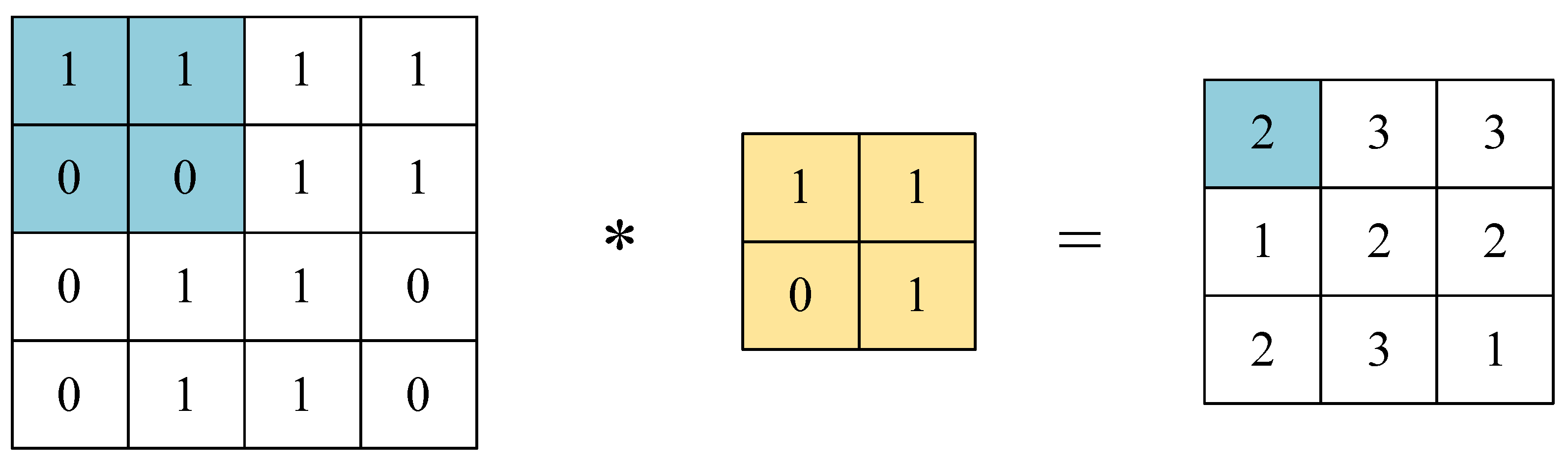
- Convolutional layer
- (2)
- Pooling layer
- (3)
- Fully connected layer
- (4)
- Activation function
2.2. Evaluation Indicators of Semantic Segmentation
2.3. Analysis of the Principle of Atrous Convolution
- (1)
- Receptive field
- (2)
- Dilated Convolutions
2.4. An ESNet for Semantic Segmentation
- (1)
- Hybrid residual block of atrous factorized convolutional encode
- (2)
- Up-sampling module and down-sampled module
3. Experiment and Results Analysis
3.1. Experimental Configurations
3.2. Experimental Configurations
3.3. Comparison of Model Experiments
3.3.1. Experimental Results and Analysis on the Cityscapes Dataset
3.3.2. Experimental Results and Analysis on the CamVid Dataset
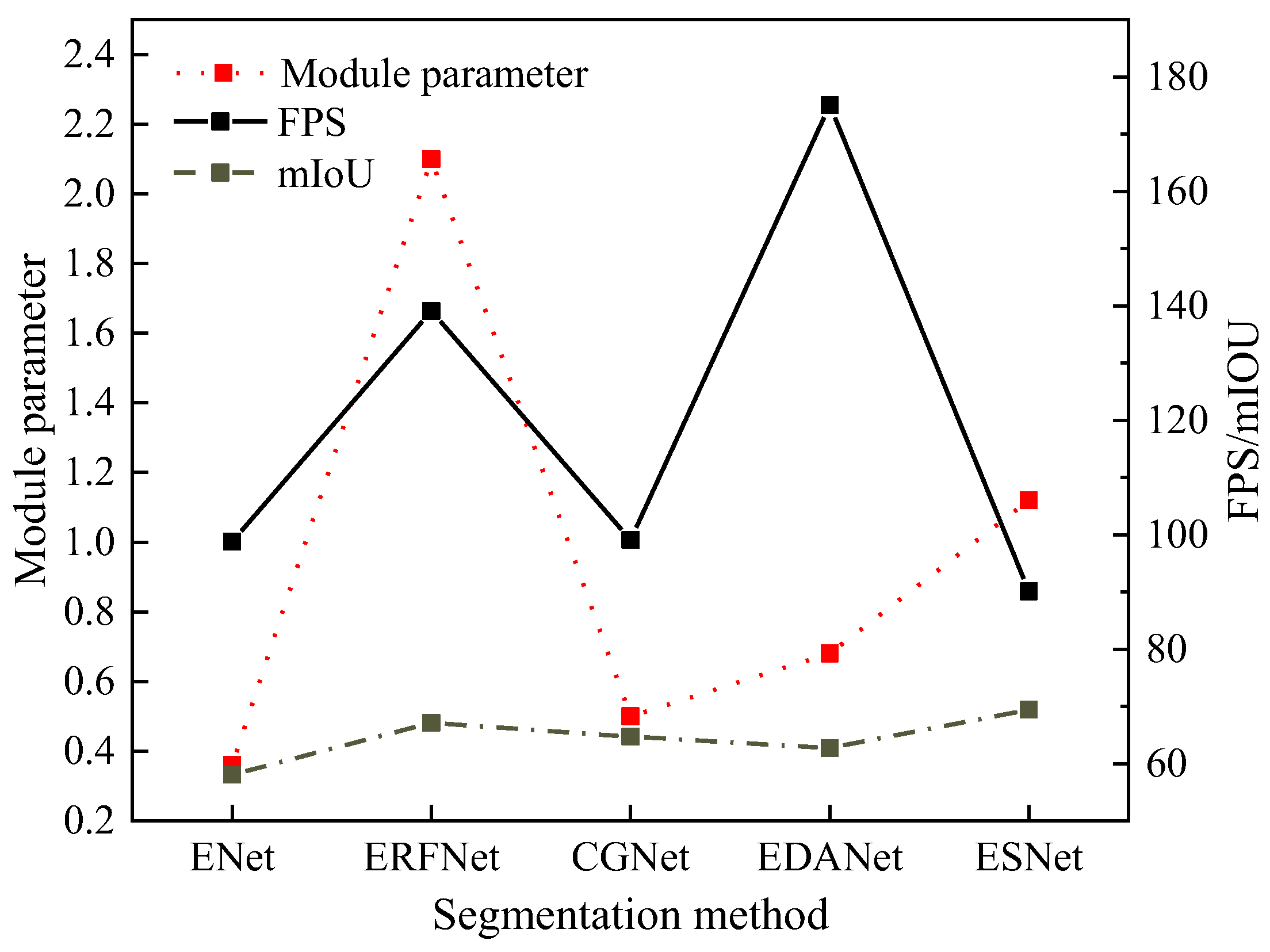
3.3.3. Efficiency of Scene Semantic Segmentation in Different Networks
3.4. Discussion
4. Conclusions
Author Contributions
Funding
Institutional Review Board Statement
Informed Consent Statement
Data Availability Statement
Acknowledgments
Conflicts of Interest
References
- Koul, S.; Eydgahi, A. Utilizing Technology Acceptance Model (TAM) for driverless car technology Adoption. J. Technol. Manag. Innov. 2018, 13, 37–46. [Google Scholar] [CrossRef] [Green Version]
- Baumann, M.F.; Brandle, C.; Zimmer-Merkle, S. The driver in the driverless car: How our technology choices will create the future. Appl. Mobilities 2019, 4, 251–255. [Google Scholar] [CrossRef]
- Dias, T.G. Driverless Cars—Another Piece of The Puzzle: Comments on “Driverless Cars will Make Passenger Rail Obsolete” by Yair Wiseman [Opinion]. IEEE Technol. Soc. Mag. 2019, 38, 36–38. [Google Scholar] [CrossRef]
- Kermany, D.S.; Goldbaum, M.; Ca, I.W.; Valentim, C.C.S.; Liang, H.; Baxter, S.L.; McKeown, A.; Yang, G.; Wu, Y.; Yan, F.; et al. Identifying Medical Diagnoses and Treatable Diseases by Image-Based Deep Learning. Cell 2018, 172, 1122–1131.e9. [Google Scholar] [CrossRef] [PubMed]
- Akhtar, N.; Mian, A. Threat of Adversarial Attacks on Deep Learning in Computer Vision: A Survey. IEEE Access 2018, 6, 14410–14430. [Google Scholar] [CrossRef]
- Kemker, R.; Salvaggio, C.; Kanan, C. Algorithms for semantic segmentation of multispectral remote sensing imagery using deep learning. ISPRS J. Photogramm. Remote Sens. 2018, 145, 60–77. [Google Scholar] [CrossRef] [Green Version]
- Zhang, Z.; Fang, W.; Du, L. Semantic Segmentation of Remote Sensing Image Based on Encoder-Decoder Convolutional Neural Network. Acta Opt. Sin. 2020, 40, 0310001. [Google Scholar] [CrossRef]
- Garg, R.; Kumar, A.; Bansal, N.; Prateek, M.; Kumar, S. Semantic segmentation of PolSAR image data using advanced deep learning model. Sci. Rep. 2021, 11, 15365. [Google Scholar] [CrossRef] [PubMed]
- Sharifi, A. Flood mapping using relevance vector machine and SAR data: A case study from Aqqala, Iran. J. Indian Soc. Remote Sens. 2020, 48, 1289–1296. [Google Scholar] [CrossRef]
- Sharifi, A. Development of a method for flood detection based on Sentinel-1 images and classifier algorithms. Water Environ. J. 2021, 35, 924–929. [Google Scholar] [CrossRef]
- Verma, A.K.; Nagpal, S.; Desai, A.; Sudha, R. An efficient neural-network model for real-time fault detection in industrial machine. Neural Comput. Appl. 2021, 33, 1297–1310. [Google Scholar] [CrossRef]
- Liu, X.; Zhao, X.; Wang, S. Blind sidewalk segmentation based on the lightweight semantic segmentation network. J. Phys. Conf. Ser. 2021, 1976, 012004. [Google Scholar] [CrossRef]
- Liu, W.; Zhou, W.; Luo, T. Cross-Modal Feature Integration Network for Human Eye-Fixation Prediction in RGB-D Images. IEEE Access 2020, 8, 202765–202773. [Google Scholar] [CrossRef]
- Hou, Y.; Li, Z.; Wang, P.; Li, W. Skeleton Optical Spectra-Based Action Recognition Using Convolutional Neural Networks. IEEE Trans. Circuits Syst. Video Technol. 2018, 28, 807–811. [Google Scholar] [CrossRef]
- Liu, N.; Han, J.; Liu, T.; Li, X. Learning to Predict Eye Fixations via Multiresolution Convolutional Neural Networks. IEEE Trans. Neural Netw. Learn. Syst. 2018, 29, 392–404. [Google Scholar] [CrossRef] [PubMed]
- Khosravi, P.; Kazemi, E.; Imielinski, M.; Elemento, O.; Hajirasouliha, I. Deep Convolutional Neural Networks Enable Discrimination of Heterogeneous Digital Pathology Images. EBio Med. 2018, 27, 317–328. [Google Scholar] [CrossRef] [PubMed] [Green Version]
- Yuan, Q.; Wei, Y.; Meng, X.; Shen, H.; Zhang, L. A Multiscale and Multidepth Convolutional Neural Network for Remote Sensing Imagery Pan-Sharpening. IEEE J. Sel. Top. Appl. Earth Obs. Remote Sens. 2018, 11, 978–989. [Google Scholar] [CrossRef] [Green Version]
- Hou, J.C.; Wang, S.S.; Lai, Y.H.; Tsao, Y.; Chang, H.-W.; Wang, H.-M. Audio-Visual Speech Enhancement Using Multimodal Deep Convolutional Neural Networks. IEEE Trans. Emerg. Top. Comput. Intell. 2018, 2, 117–128. [Google Scholar] [CrossRef] [Green Version]
- Chen, J.; Liu, Z.; Wang, H.; Nunez, A.; Han, Z. Automatic Defect Detection of Fasteners on the Catenary Support Device Using Deep Convolutional Neural Network. IEEE Trans. Instrum. Meas. 2018, 67, 257–269. [Google Scholar] [CrossRef] [Green Version]
- Jia, F.; Lei, Y.; Lu, N.; Xing, S. Deep normalized convolutional neural network for imbalanced fault classification of machinery and its understanding via visualization. Mech. Syst. Signal Processing 2018, 110, 349–367. [Google Scholar] [CrossRef]
- Ang, L.L.; Hacer, Y.K. Foreground Segmentation Using a Triplet Convolutional Neural Network for Multiscale Feature Encoding. Pattern Recognit. Lett. 2018, 112, 256–262. [Google Scholar]
- Wang, S.H.; Phillips, P.; Sui, Y.; Liu, B.; Yang, M.; Cheng, H. Classification of Alzheimer’s Disease Based on Eight-Layer Convolutional Neural Network with Leaky Rectified Linear Unit and Max Pooling. J. Med. Syst. 2018, 42, 85. [Google Scholar] [CrossRef] [PubMed]
- Hayou, S.; Doucet, A.; Rousseau, J. On the Selection of Initialization and Activation Function for Deep Neural Networks. J. Fuzhou Univ. 2018, 56, 1437–1443. [Google Scholar]
- Xu, D.; Tan, M. Multistability of delayed complex-valued competitive neural networks with discontinuous non-monotonic piecewise nonlinear activation functions. Commun. Nonlinear Sci. Numer. Simul. 2018, 62, 352–377. [Google Scholar] [CrossRef]
- Chandrasekaran, S.T.; Jayaraj, A.; Karnam, V.; Banerjee, I.; Sanyal, A. Fully Integrated Analog Machine Learning Classifier Using Custom Activation Function for Low Resolution Image Classification. IEEE Trans. Circuits Syst. I 2021, 68, 1023–1033. [Google Scholar] [CrossRef]
- Jbf, A.; Rms, B.; Jab, A. Dynamic interactive theory as a domain-general account of social perception—ScienceDirect. Adv. Exp. Soc. Psychol. 2020, 61, 237–287. [Google Scholar]
- Sadakata, M.; Weidema, J.L.; Honing, H. Parallel pitch processing in speech and melody: A study of the interference of musical melody on lexical pitch perception in speakers of Mandarin. PLoS ONE 2020, 15, e0229109. [Google Scholar] [CrossRef]
- Sobran, M.A.; Cotter, P.A. The BvgS PAS Domain, an Independent Sensory Perception Module in the Bordetella bronchiseptica BvgAS Phosphorelay. J. Bacteriol. 2019, 201, e00286-19. [Google Scholar] [CrossRef] [Green Version]
- Li, J.; Huang, H.; Zhu, M.; Huang, S.; Zhang, W.; Dinesh-Kumar, S.; Tao, X. A Plant Immune Receptor Adopts a Two-Step Recognition Mechanism to Enhance Viral EffectorPerception. Mol. Plant 2019, 12, 248–262. [Google Scholar] [CrossRef] [PubMed] [Green Version]
- Li, J.; Yang, H. The underwater acoustic target timbre perception and recognition based on the auditory inspired deep convolutional neural network. Appl. Acoust. 2021, 182, 108210. [Google Scholar] [CrossRef]
- Moreno, I.; Davis, J.A.; Gutierrez, B.K.; Sánchez-López, M.M.; Cottrell, D.M. Multiple-order correlations and convolutions using a spatial light modulator with extended phase range. Opt. Lasers Eng. 2021, 146, 106701. [Google Scholar] [CrossRef]
- Witt, H.J.; Atrio-Barandela, F. Fast Computational Convolution Methods for Extended Source Effects in Microlensing Light Curves. Astrophys. J. 2019, 880, 152. [Google Scholar] [CrossRef] [Green Version]
- Ren, H.; Yu, X.; Zou, L.; Zhou, Y.; Wang, X.; Bruzzone, L. Extended convolutional capsule network with application on SAR automatic target recognition. Signal Processing 2021, 183, 108021. [Google Scholar] [CrossRef]
- Liu, Y.Y.; Yan, Y.M.; Xu, M.; Song, K.; Shi, Q. Exact generator and its high order expansions in the time-convolutionless generalized master equation: Applications to the spin-boson model and exictation energy transfer. Chin. J. Chem. Phys. 2018, 31, 575–583. [Google Scholar] [CrossRef]
- Ying, S.; Zhang, X.; Xin, Q.; Huang, J. Developing a multi-filter convolutional neural network for semantic segmentation using high-resolution aerial imagery and LiDAR data. ISPRS J. Photogramm. Remote Sens. 2018, 143, 3–14. [Google Scholar]
- Yang, T.; Wu, Y.; Zhao, J.; Guan, L. Semantic Segmentation via Highly Fused Convolutional Network with Multiple Soft Cost Functions. Cogn. Syst. Res. 2018, 53, 20–30. [Google Scholar] [CrossRef] [Green Version]
- Lentz, D.L.; Hamilton, T.L.; Dunning, N.P.; Tepe, E.J.; Scarborough, V.L.; Meyers, S.A.; Grazioso, L.; Weiss, A.A. Environmental DNA reveals arboreal cityscapes at the Ancient Maya Center of Tikal. Sci. Rep. 2021, 11, 12725. [Google Scholar] [CrossRef]
- Nanda, A. Of cityscapes, affect and migrant subjectivities in Kiran Desai’s Inheritance of Loss. Subjectivity 2021, 14, 119–132. [Google Scholar] [CrossRef]
- Wen, L.; He, L.; Gao, Z. Research on 3D Point Cloud De-Distortion Algorithm and Its Application on Euclidean Clustering. IEEE Access 2019, 7, 86041–86053. [Google Scholar] [CrossRef]


| SegNet | ENet | ESPNet | CGNet | ERFNet | ICNet | EDANet | ESNet | |
|---|---|---|---|---|---|---|---|---|
| Daytime scene | 67.5 | 38.6 | 9.6 | 25.1 | 25.7 | 40.0 | 21.2 | 20.8 |
| Night scene | 43.2 | 30.0 | 9.1 | 21.6 | 24.5 | 37.2 | 20.8 | 19.6 |
| In rainy weather | 60.0 | 33.8 | 9.4 | 24.5 | 23.5 | 38.6 | 21.6 | 20.4 |
| Average value | 56.9 | 34.1 | 9.3 | 23.8 | 24.6 | 38.6 | 21.2 | 20.3 |
Publisher’s Note: MDPI stays neutral with regard to jurisdictional claims in published maps and institutional affiliations. |
© 2022 by the authors. Licensee MDPI, Basel, Switzerland. This article is an open access article distributed under the terms and conditions of the Creative Commons Attribution (CC BY) license (https://creativecommons.org/licenses/by/4.0/).
Share and Cite
Li, Y.; Shi, J.; Li, Y. Real-Time Semantic Understanding and Segmentation of Urban Scenes for Vehicle Visual Sensors by Optimized DCNN Algorithm. Appl. Sci. 2022, 12, 7811. https://doi.org/10.3390/app12157811
Li Y, Shi J, Li Y. Real-Time Semantic Understanding and Segmentation of Urban Scenes for Vehicle Visual Sensors by Optimized DCNN Algorithm. Applied Sciences. 2022; 12(15):7811. https://doi.org/10.3390/app12157811
Chicago/Turabian StyleLi, Yanyi, Jian Shi, and Yuping Li. 2022. "Real-Time Semantic Understanding and Segmentation of Urban Scenes for Vehicle Visual Sensors by Optimized DCNN Algorithm" Applied Sciences 12, no. 15: 7811. https://doi.org/10.3390/app12157811