3D JPS Path Optimization Algorithm and Dynamic-Obstacle Avoidance Design Based on Near-Ground Search Drone

Featured Application

This research can be applied to path planning and automatic obstacle avoidance of drone in low altitude complex environments.

Abstract

As various fields and industries have progressed, the use of drones has grown tremendously. The problem of path planning for drones flying at low altitude in urban as well as mountainous areas will be crucial for drones performing search-and-rescue missions. In this paper, we propose a convergent approach to ensure autonomous collision-free path planning for drones in the presence of both static obstacles and dynamic threats. Firstly, this paper extends the jump point search algorithm (JPS) in three dimensions for the drone to generate collision-free paths based on static environments. Next, a parent node transfer law is proposed and used to implement the JPS algorithm for any-angle path planning, which further shortens the planning path of the drones. Furthermore, the optimized paths are smoothed by seventh-order polynomial interpolation based on minimum snap to ensure the continuity at the path nodes. Finally, this paper improves the artificial potential field (APF) method by a virtual gravitational field and 3D Bresenham’s line algorithm to achieve the autonomous obstacle avoidance of drones in a dynamic-threat conflict environment. In this paper, the performance of this convergent approach is verified by simulation experiments. The simulation results show that the proposed approach can effectively solve the path planning and autonomous-obstacle-avoidance problems of drones in low-altitude flight missions.

1. Introduction

Initially, drones were valued by the military industries of various countries because of their stealth, relatively low cost, ease of operation, and lack of fear of casualties. Nowadays, the use of drones is gradually spreading from military [1] to education, film and television [2], agriculture [3], and service industries [4]. Drones are also known as flying robots or unmanned aerial vehicles [5]. Most of these vehicles are used for observation, search, and discreet planning [6]. Recent advances in UAV technology have made it possible to perform near-ground search and rescue (SAR) in complex environments such as urban and mountainous areas [7]. For example, during a rescue mission in Oregon, drones were used to identify fatalities in the Narrows Canyon and eliminate the need for search-and-rescue personnel to perform dangerous rope drops at night [8]. This technology can greatly reduce the search time, improve the efficiency of the rescue, and provide guidance assistance to teams in areas where manual patrols are difficult and time-consuming [9]. For now, drones still have very limited airspace activity in some areas, as shown in Figure 1. Missions in the no-fly zone require even more authorization and permission from the relevant authorities [10]. However, this would highly limit the scope of drone search and rescue and would not bring out the strengths and working standards of drones. Rational establishment and planning of the framework of drone-based search-and-rescue systems and the proper use of drones in urban and mountainous areas for near-ground search missions will provide great help to rescue [11].

Unlike other commercial aircraft, the short takeoff and landing of drones in the vertical direction increases the suitability of drones for near-ground search among complex environments [12]. Nonetheless, drones still face significant challenges in performing search-and-rescue missions in the near field. At present, drone-based near-ground search and rescue usually has a similar set of constraints. First, the search time is tight and drones need to arrive at the mission site as quickly as possible, and any delay could lead to irreversible and serious consequences [13]. Secondly, the working environment is not friendly, and the drone has more complex scenes such as buildings and forests during low-altitude operations, which leads to an excessive number of total turning angles in the path generated by the drone. It is not only energy-consuming, but also increases the search time [14]. Third, due the dynamic threats that arise during the execution of the mission, the drones need to maintain a safe distance between the working environment and other dynamic obstacles [15,16] to prevent the phenomenon of course conflict. These unfavorable constraints make it difficult for drones to complete missions in urban as well as mountainous low-altitude airspace.

In order to solve the above-mentioned problems, this paper reduces the total length of the drone’s generated path and the total turning angle of the path by introducing an any-angle path-planning strategy [17] and a path-smoothing technique [18] to reduce the time required and energy consumption for flight. Secondly, for dynamic threats in the mission environment, stable dynamic-obstacle avoidance techniques need to be introduced [19]. This is to avoid collision phenomena caused by possible obstacle changes and other drones’ flight path conflicts in the complex operating environment.

2. Related Work

Path planning, a key element of autonomous drone navigation, is actually the selection of a shortest obstacle-avoidance path from the starting point to the target point within the flight area. Its essence is the problem of finding the optimal solution of the path [20]. The feasibility constraints and dynamic threats that occur in the operational airspace should be fully considered in the path-planning process of drones [21]. More precisely, the resultant path generated by the path planning of the drones should be the optimal path that satisfies the dynamic-threat avoidance condition.

In previous research, various algorithms have been developed for dynamic-obstacle-avoidance design. In the paper [22], a method based on the combination of D* Lite and a probabilistic roadmap (RPM) is proposed to implement the path planning of drones. The article constructs the initialized node roadmap by RPM using random sampling and then uses D*lite for local corrections. For grid-discretized maps, local modification based on initialized paths is a simple and effective method. Local modifications can avoid global path corrections due to obstacle changes [23]. However, if there are many dynamic obstacles in the workspace, frequent local modifications will lead to a significant decrease in the computational efficiency of the algorithm. In addition, the poor smoothness of the path can also have a negative effect on the efficiency of the drones and their energy consumption.

Model predictive control (MPC) is an online-based optimal control strategy that is often used for trajectory tracking [24] and dynamic-obstacle avoidance [25] of drones and mobile robot. MPC relies on historical information and future inputs of objects in the finite time domain and predicts their future outcomes by means of predictive models of the objects [26]. MPC is different from the optimal-control method (OCM) [27]. The OCM tends to emphasize the optimality of the results, thus making it difficult to solve for nonlinear cases containing complex constraints. Instead, MPC adopts a compromise strategy that is more supportive of nonlinear systems, but sacrifices optimality to some extent. In the article [28], a nonlinear, nonconvex solver based on proximal averaged Newton for optimal control (PANOC) and fusing penalty functions is proposed to implement drone navigation and obstacle avoidance. However, MPC requires a high accuracy of the model [29], and the accuracy of the model has a very high impact on the performance of the MPC results. The modeling problem is too complex for hybrid systems with complex objects, such as unmanned aircraft systems.

The artificial potential field (APF) method is a virtual-force approach proposed by Khatib [30]. A safe and smooth path is easily obtained by introducing an artificial potential field [31]. The basic idea of the artificial-potential-field method is to control the drone’s movement by the combined force generated by the virtual gravitational field at the target location and the virtual repulsive field around the obstacle. The APF method is more intuitively defined than other methods, has a simple model structure, and does not require a large amount of computation to achieve real-time obstacle avoidance and complete the path-planning task [32]. On the other hand, the APF method has low objective reachability due to the drawback of local optimal solutions. To solve such a problem, the paper [33] used the random generation of virtual target points within a local field of very small points to break the equilibrium of gravitational and repulsive forces and bring the drones out of the local-optimum point. This approach ensures the safety and accessibility of the path-planning process to a large extent; however, it neglects the path quality issue.

In recent years, jump point search methods (JPS) using heuristic search methods have been proposed, driven by the efficiency of path-planning algorithms [34]. The classical JPS algorithm builds on the framework of the A* algorithm and further optimizes the way of finding successor nodes through the neighbor-pruning rule and forced neighbors, which improves the search efficiency of the A* algorithm [35] and, thus, greatly reduces the time consumption in the search process [36]. From another perspective, the JPS algorithm based on discrete grid maps also has many problems. During the pathfinding process performed by the JPS algorithm, the planning usually starts from the center of the grid and only allows expansion to the centroids of neighboring grids, as shown in Figure 2. This will result in a fixed direction of search for the JPS algorithm, ignoring path selection at any angle [37], which leads to a longer resultant path than the actual path. Secondly, the JPS algorithm is mainly used for pathfinding in static space. For dynamic threats and changes in the path-planning environment, JPS algorithms can only be solved using replanning, which will significantly increase the time cost of path planning [38] and is not conducive to drones’ mission execution.

Based on the above issues and inspired by previous related work, this proposal takes into account the time cost of path planning for drones, the degree of path smoothing (path length and total path-turning angle), and obstacle avoidance strategies for static obstacles and dynamic threats. First, this paper extends the traditional JPS to the 3D space and implements the any-angle path planning of the 3D JPS algorithm by the parent node transfer law, which ensures that the resultant path of the JPS algorithm is optimal in terms of length and total turning-angle measures. Secondly, this paper introduces the polynomial-interpolation method based on minimum snap to achieve the continuity and smoothness of the position, velocity, acceleration, and jerk function at the drones’ path nodes while ensuring the shortest path. Finally, this paper uses the 3D Bresenham’s line algorithm and the virtual-target gravitational field to solve the disadvantages of the artificial-potential-field method which is easy to fall into the minima, and combines the 3D JPS algorithm to realize the drones’ real-time dynamic-obstacle avoidance.

The main contributions of this paper are listed below. First, this paper achieves efficient autonomous pathfinding for drones in a static environment through JPS 3D extension. Secondly, the generation path of the JPS algorithm is further optimized by the parent node transfer law and polynomial-interpolation optimization. Finally, a dynamic-obstacle avoidance scheme based on the improved artificial-potential-field method is proposed to realize the safe flight of drones in the dynamic environment of low-altitude airspace.

3. Path-Planning Design and Dynamic-Obstacle Avoidance Strategy

For drones performing near-ground search missions, feasible path planning should integrate path quality and real-time obstacle avoidance capabilities. A safe and reliable autonomous-obstacle-avoidance path is planned under the condition of ensuring the shortest path and the best quality. The proposed path optimization method and the dynamic-obstacle-avoidance strategy are based on the global set of path nodes derived from the 3D JPS algorithm, as shown in Figure 3.

3.1. Global Path-Planning Design Based on 3D JPS Algorithm

The JPS algorithm is a global path-planning algorithm based on a discrete grid map model in a static environment. In general, static obstacles in the initial drone flight airspace are relatively easy to obtain or the static obstacles themselves are known. Therefore, this paper develops a 3D jump point search algorithm based on the original JPS algorithm for the generation of global paths for drones in a static initial environment.

3.1.1. Traditional JPS Algorithm

The JPS algorithm was proposed by Harabor and Grastien in 2011 [34]. The main idea of the JPS algorithm is to further optimize the process of finding subsequent path nodes by the A* algorithm based on the heuristic function of the A* algorithm through the neighbor-pruning rule and the forced-neighbor judgment method. The JPS algorithm drastically reduces the number of nodes that need to be accessed in the openlist list, reducing the time and space costs of the algorithm, as shown in Figure 4. The light-gray grid indicates the nodes that have been visited by the openlist, and the purple grid indicates the remaining nodes in the current openlist.

The direction of expansion of the JPS algorithm during path planning depends on the orientation of the natural neighbors given by the neighbor-pruning rule. When JPS extends the path in a particular direction, it identifies a set of natural neighbors among the neighboring nodes evaluated by the neighbor-pruning rule. If the extension direction is a straight line, the natural neighbor of the current grid is defined as the next node in the same direction, as shown in Figure 5a. That is, JPS will continue searching along the direction of the current natural neighbor. When the extension direction is diagonal, the natural neighbors of the current grid are the next node along the extension diagonal and the vertical and horizontal nodes in the extension direction, as shown in Figure 5b. JPS will start expanding along the natural neighbors in the vertical and horizontal directions until they are blocked or a jump point is found before considering the search in the diagonal direction. If there is an obstacle among the pruned neighbors, this will make it impossible to prune all unnatural neighbors. The grids that are forced to become natural neighbors as a result of this phenomenon are called forced neighbors, as shown in Figure 5c,d.

In essence, JPS is a heuristic search algorithm that relies on jump points for path planning. The efficiency of the JPS algorithm is inextricably linked to the choice of jump points. Usually, the identification of jump points for the JPS algorithm relies on the judgment of forced neighbors. The current node is the jump point if it is the start point, the target point, or if there is at least one forced neighbor. If the current node is a diagonal search and there is a jump point in its horizontal or vertical direction, the current node is also the same as the jump point.

The JPS algorithm is much lower than the A* algorithm in terms of time complexity. The fundamental reason is that the openlist list of the JPS algorithm no longer stores all the natural neighbors of the current node, but the jump nodes that play a key role in the final generated path. Although the JPS algorithm and the A* algorithm generate paths of equal length, the A* algorithm requires far more nodes to be computed and visited than the JPS algorithm, which explains why the JPS algorithm is more efficient than A*. In particular, the efficiency of the JPS algorithm is more significant in complex environments. Just as the results tested by Harabor are consistent, the search speed of the JPS algorithm is an order of magnitude higher than that of the A* algorithm [34]. Therefore, choosing the JPS algorithm to perform the drone path planning has a general advantage in meeting the requirements of efficiency.

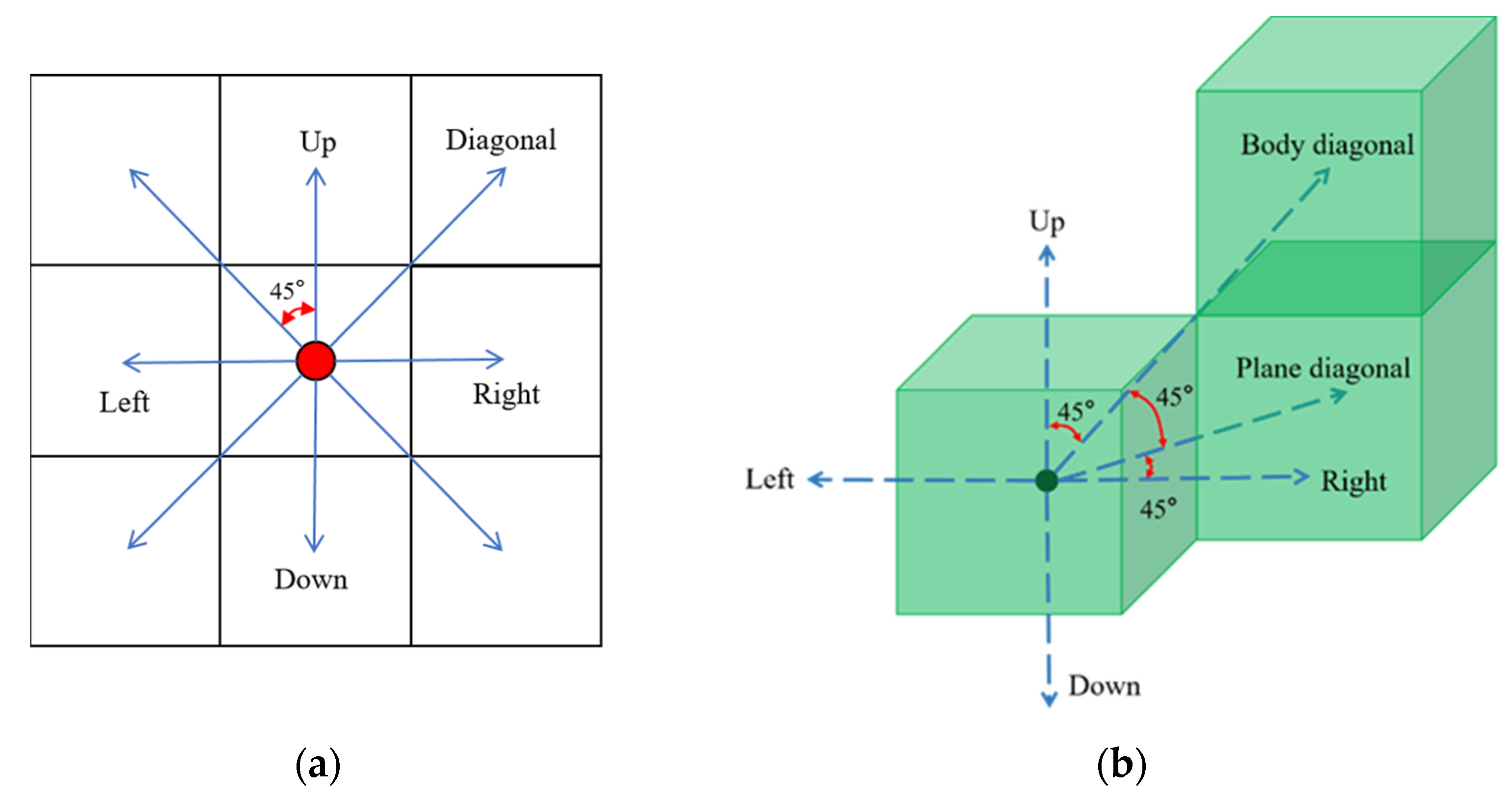
3.1.2. 3D Extension of JPS Algorithm

In order to ensure that the drone maintains excellent static-obstacle-avoidance capability during the search mission in low-altitude airspace, this paper extends the JPS algorithm in three dimensions.

In the traditional 2D space, the JPS algorithm uses a single grid node as the smallest unit and the current node and contains all eight neighboring nodes as the smallest set for path-planning search and judgment. The number of neighbors and the orientation of the current node play a crucial role in the search direction of the JPS algorithm, as shown in Figure 6a. The minimum set of the current node and all its neighbors included in the expansion process of 3D JPS is different from the traditional JPS algorithm. The neighboring nodes of the current node are expanded in 3D space as 26 belonging grid nodes directly connected to the current node, as shown in Figure 6b. In Figure 6b, only the expansion direction of the same plane and the expansion of one edge of each of the upper and lower planes are given; all other directions can be obtained by rotation.

The result of the change in the minimum set in the 3D space is a difference in the direction of the expansion of the JPS algorithm during the path-planning process. The different expansion directions are determined by the neighbor-pruning method of the JPS algorithm. Therefore, this paper makes further modifications to the neighbor-pruning rule for 3D JPS as follows.

• The parent node $parent(x)$ of the current node $x$ satisfies the two-dimensional pruning rule when it is in the same plane as the current node with linear extension and does not involve other planes, as shown in Figure 7a. The current node needs to prune off any neighbor node in the same plane that satisfies the following constraint $n$:

  $$len(<parent(x),....,n>\backslash x)\le len(<parent(x),x,n>)$$

  (1)

  where the $len$ function represents the distance between nodes, and $<parent(x),....,n>\backslash x$ represents the set of all nodes that reach $n$ from the $parent(x)$ node without the current node $x$.
• The parent node $parent(x)$ of the current node $x$ and the current node in the same plane diagonal expansion also satisfies the two-dimensional pruning rule, and does not involve other planes, as shown in Figure 7b. That is, it is necessary to prune off any neighbor node $n$ in the same plane that satisfies the following constraint:

  $$len(<parent(x),....,n>\backslash x)<len(<parent(x),x,n>)$$

  (2)
• If the parent node $parent(x)$ of the current node $x$ and the current node for the body diagonal expansion, the need to expand along the diagonal direction to the upper level while satisfying the formula (b), as shown in Figure 7c.

From another point of view, forced neighbors and jump points are a relative set of concepts in the 3D JPS algorithm. The number and location of forced neighbors has an intuitive effect on jump points. We assume that the set of pruned neighbors is $P=<x_1,x_2,x_3\dots ,x_n>$ in a minimal set with the current grid $x$ as the core. There exists an obstacle $x_{ob}\in P$; if there exists any neighbor grid $x_i\in P,x_i\ne x_{ob}$ of $x_{ob}$ satisfying the following condition, then $x_i$ is called a forced neighbor of the current node $x$. Additionally, $x$ is called the jump point.

$$len(<parent(x),x,n>)<len(<parent(x),\dots ,n>\backslash x)$$

(3)

The JPS paths are generated in the 3D space consisting of a 3D grid, following an expansion from straight lines to diagonals in the same plane and then to diagonals in the body. In the process of expanding the 3D JPS, the current node is used as the reference, and the first three linear-search directions parallel to the x-axis, y-axis, and z-axis are expanded, as shown in Figure 8a. The same-plane diagonal expansion is performed only when no jump point is found in the linear direction and the same-plane expansion follows the two-dimensional JPS algorithm expansion rules, as shown in Figure 8b. If the jump point is still not found, the final body diagonal expansion is performed; that is, a grid is expanded along the diagonal of the map body and the linear and planar search is continued, as shown in Figure 8c.

In the process of 3D JPS algorithm path planning, openlist and closelist are used to record the search process, where the openlist list stores the candidate jump points in the current search. After computing the heuristic function for each candidate jump point, the point with the smallest heuristic function value is taken from the openlist and added to the closelist for this round. During the next round of search, this jump point is used as the parent of the current node to continue the search until the target is reached. The heuristic function of the 3D JPS algorithm is shown below.

$$f(x)=g(x)+h(x)$$

(4)

where $x$ denotes the current node and $g(x)$ denotes the actual cost from the initial node to the current node $x$. $h(x)$ denotes the heuristic evaluation cost of reaching the target point $goal$ from the current node $x$. In general, the three-dimensional spatial Euclidean distance formula is used for evaluation, which is shown below.

$$dist(x,goal)=\sqrt{{(x_x-goa{l}_x)}^2+{(x_y-goa{l}_y)}^2+{(x_z-goa{l}_z)}^2}$$

(5)

In this paper, the path-planning steps of the 3D JPS algorithm are shown below.

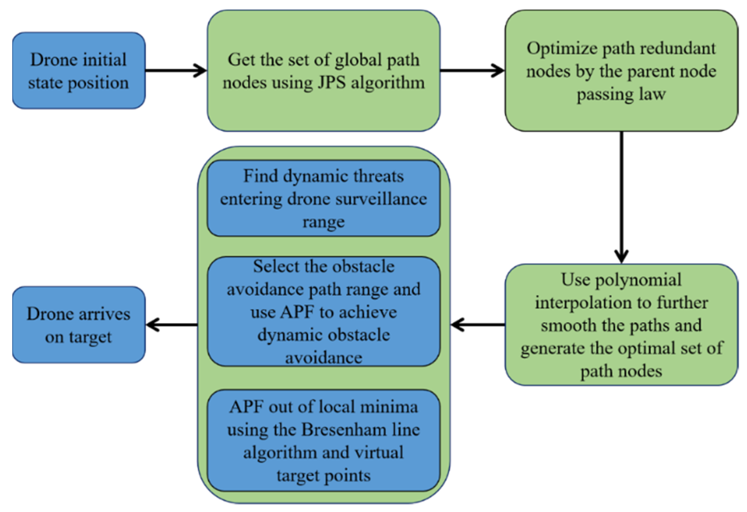
• Initialize the static spatial environment and discretize the drone flight area into a grid model.
• Set the initial position of the drone to $x_{start}$ and the target point $x_{end}$ and add $x_{start}$ to the openlist.
• The neighbor-pruning rule is selected according to the position information of the current node and its parent node, and the expansion direction of the current node is calculated.
• Find jump points by forcing the location of neighbors and add them to the openlist.
• Each node in the openlist is computed by a heuristic function. The node with the smallest computed value is selected as the jump point and the parent node for the next search process.
• Add the nodes that play the role of parent nodes in this search process to the closelist. If there is $x_{end}$ , the search will be terminated, and the search path will be formed by the list of closelist. If $x_{end}$ is not present, repeat steps 3 through 6.

3.2. Trajectory Optimization Based on the Resultant Path of 3D JPS Algorithm

The 3D JPS algorithm is a path planning algorithm based on a discrete 3D grid map. The paths obtained directly from the 3D JPS algorithm still cannot escape the limitations imposed by the search direction. This will cause the 3D JPS algorithm to ignore the possibility of any search directions during the search process, making the path appear unnecessarily twisted and unsmooth. In this paper, the set of path nodes of the 3D JPS algorithm is optimized by the parent node transfer law, and the redundant nodes are removed to realize the JPS algorithm for any-angle path planning. Meanwhile, the minimum-snap seventh-order polynomial-interpolation method is introduced to further ensure the continuity and smoothness of information such as path node position, velocity, acceleration, and jerk function of the drone in the flight process. The trajectory optimization framework based on the 3D JPS algorithm for path generation is shown in Figure 9.

3.2.1. An Any-Angle Path-Planning Strategy Based on the Parent Node Transfer Law

In the traditional JPS algorithm for path planning, the expansion direction of the current node is determined by the neighbor-pruning law. The selection of the neighbor-pruning rule, on the other hand, relies on the position relationship of the parent node with respect to the current node. In general, the final path result set generated by the JPS algorithm contains a chain of parent–child node relationships. After the JPS algorithm completes the search, it is also necessary to infer the final path based on the chain of parent–child node relationships. The parent–child node relationship chains obtained by the JPS algorithm and the A* algorithm are different. The relational chain of the A* algorithm is complete, and it completely covers every grid node in the result path searched by the A* algorithm. As for the JPS algorithm, it is obvious that the chain of relations consists of jump points and the redundant nodes between every two jump points are removed, as shown in Figure 10.

From the complete chain of relations, it can be found that the parent of any node $x$ can only be a visible neighbor node of $x$, as shown by $parent{(x)}_{old}$ in Figure 10. The JPS algorithm, however, breaks this rule. It can be seen that the parent node in the parent–child node relationship chain obtained by the JPS algorithm is not a neighbor of the parent node, but has direct visibility between the two nodes, that is, the line of sight (LOS) has direct accessibility [17]. When two nodes have a parent–child relationship, the redundant nodes in their middle can be deleted, as is the case with the 3D JPS algorithm. Therefore, in this paper, the way of passing the parent node to the forward node in the parent–child node relationship chain is called the parent-node-passing law, and it is further improved and expanded on this basis.

The JPS algorithm and the 3D JPS algorithm still have a gap between the obtained paths compared to the shortest paths in the actual space. The fundamental reason for this is the limitation of the search direction, as shown in Figure 11.

As we can see in Figure 11, there are still redundant steering points in the set of nodes for both JPS algorithms resulting in paths that are not the shortest. Therefore, how to delete these redundant nodes becomes the key to path optimization. The core of the parent-passing rule is that if there is LOS reachability between two nodes, all nodes between these two nodes are considered redundant, and any unnecessary path transitions caused by them can be replaced by the direct connection of the two nodes. It would be unwise to use the strategy of combining every two nodes to verify the LOS reachability in the parent-node-passing rule. As the number of path nodes grows, the number of such verifications will increase significantly to affect the overall computational efficiency of the algorithm. For this reason, an inert strategy is used in this paper in the specific implementation of the parent-node-passing law. By default, all nodes have LOS reachability with the parent node of the current detection point, and LOS authenticity is considered when a specific verification of a node in the path is needed. The specific way of the parent-node-passing law used in this paper is as follows.

• First of all, the path nodes of the 3D JPS algorithm are complemented so that each raster through which the path of the 3D JPS algorithm passes is included in the set of nodes. Let the set of nodes be $pathlist=<x_{end},x_n,x_{n-1},\dots ,x_i,\dots ,x_1,x_{start}>$.
• Set the parent node of all nodes in the node collection to be the initial node. That is, all nodes have direct visibility with the initial node by default.
• Since the parent–child relationship between node $x_1$ and $x_{start}$ is not modified, it is only necessary to perform LOS reachability detection with $x_{start}$ from node $x_2$ to node $x_{end}$ in order to verify whether the visibility between nodes holds.
• If visibility holds, the node between the current node and $x_{start}$ will be deleted and added to the deletelist without changing the parent node relationship.
• If visibility does not hold, the parent node for the current node needs to be found again in the deletelist, and the parent node of the remaining nodes without LOS detection is replaced with the parent node of the current node to continue the detection.
• When the parent node of $x_{end}$ is passed, the algorithm ends and the shortest path is output.

In this paper, the pseudocode of the parent-node-passing rule is shown as follows (Algorithm 1).

Algorithm 1: Parent Node Passing

3.2.2. Optimization of Trajectory Smoothing Based on Minimum-Snap Seventh-Order Polynomial Interpolation

For drones performing near-ground missions, path planning should fully take into account the feasibility constraints that arise during the actual flight of the drones. To be precise, the path obtained by the path planning algorithm of drone should meet the path space node state continuous and smooth, to achieve the shortest path. The full-state space of the drone is 12 dimensions, which are position, velocity, attitude angle, and angular velocity, as shown in Equation (6).

$$\mathrm{x}={\left[x,y,z,\varphi ,\theta ,\psi ,\dot{x},\dot{y},\dot{z},p,q,r\right]}^{\top }$$

(6)

However, in the process of drones’ path planning, it is not possible to plan for the full dimensional space because it would be very complex and difficult to compute. In their paper [38], Daniel Mellinger et al. demonstrated that the 12-dimensional full state of a drone can be represented by a flat output space composed of four-dimensional variables, as shown in Equation (7).

$$\sigma ={\left[x,y,z,\psi \right]}^{\top }$$

(7)

There are only four-dimensional variables in this space, namely, the positions of the $x$-axis, $y$-axis, $z$-axis, and yaw angle $\psi$. The remaining states can be represented by the algebra of these four variables and their finite order derivatives.

Therefore, in this paper, based on the four-dimensional flat-output space of UAV, the seventh-order polynomial based on minimum snap is selected for trajectory optimization. Additionally, for the possibility of recollision of the optimized path, the node expansion interval is used and the flight safety corridor is set by applying the inequality constraint. Using minimum snap as the optimization objective ensures the continuity of the generated paths of the 3D JPS algorithm in terms of node position, velocity, acceleration, and jerk function and further reduces the energy consumption of the drone during the mission and enhances the safety during the flight.

In order to ensure the degree of fit of the optimization curve to the original path and the flight corridor setting, firstly, this paper performs the node interpolation process for the set of nodes of the 3D JPS algorithm according to the fixed step size $step$. The interpolation method is shown in the following pseudocode (Algorithm 2).

Algorithm 2: Path node interpolation

Second, the segmentation is performed according to the number of nodes in the set of path nodes generated by the 3D JPS algorithm. Assuming that the set of nodes has n + 1 nodes, the overall path is divided into n segments. The polynomial expression for the n segment path is shown in Equation (8).

$$f\left(t\right)=\{\begin{array}{cc}{\displaystyle {\displaystyle \sum }_{i=0}^k}{p}_{1,i}{t}^i=\left(\begin{array}{cccc}{t}^0& t^1& \dots & t^k\end{array}\right){\left(\begin{array}{cccc}{p}_{1,0}& p_{1,1}& \cdots & p_{1,k}\end{array}\right)}^{\top }\hfill & \left(T_0\le t\le T_1;k=7\right)\\ {\displaystyle {\displaystyle \sum }_{i=0}^k}{p}_{2,i}{t}^i=\left(\begin{array}{cccc}{t}^0& t^1& \dots & t^k\end{array}\right){\left(\begin{array}{cccc}{p}_{2,0}& p_{2,1}& \cdots & p_{2,k}\end{array}\right)}^{\top }\hfill & \left(T_1\le t\le T_2;k=7\right)\\ ⋮& \\ {\displaystyle {\displaystyle \sum }_{i=0}^k}{p}_{m,i}{t}^i=\left(\begin{array}{cccc}{t}^0& t^1& \dots & t^k\end{array}\right){\left(\begin{array}{cccc}{p}_{m,0}& p_{m,1}& \cdots & p_{m,k}\end{array}\right)}^{\top }\hfill & \left(T_{m-1}\le t\le T_m;k=7\right)\\ ⋮& \\ {\displaystyle {\displaystyle \sum }_{i=0}^k}{p}_{n,i}{t}^i=\left(\begin{array}{cccc}{t}^0& t^1& \dots & t^k\end{array}\right){\left(\begin{array}{cccc}{p}_{n0}& p_{n,1}& \cdots & p_{n,k}\end{array}\right)}^{\top }\hfill & \left(T_{n-1}\le t\le T_n;k=7\right)\end{array}$$

(8)

where $p_{m,i}$ denotes the $i$th polynomial coefficient of the $m$th segment of the path, $t$ denotes the drone flight time, and $T_0$ to $T_n$ denote the moments when the drone passes the endpoints of each segment of the path. Next, by performing multiple derivative calculations for $f(t)$, the expressions for velocity, acceleration, jerk, and snap for the corresponding path segments are obtained, as shown in Equations (9) to (12).

$$v_m(t)=\left(\begin{array}{lllll}0& 1& 2t& \cdots & k{t}^{k-1}\end{array}\right){\left(\begin{array}{llll}{p}_{m,0}& p_{m,1}& \cdots & p_{m,k}\end{array}\right)}^{\top }$$

(9)

$$a_m(t)=\left(\begin{array}{llllll}0& 0& 2& 6t& \cdots & k(k-1)t^{k-2}\end{array}\right){\left(\begin{array}{llll}{p}_{m,0}& p_{m,1}& \cdots & p_{m,k}\end{array}\right)}^{\top }$$

(10)

$$jer{k}_m(t)=\left(\begin{array}{llll}\begin{array}{lll}0& 0& 0\end{array}& \begin{array}{ll}6& 12t^2\end{array}& \cdots & \frac{k!}{(k-3)!}{t}^{k-3}\end{array}\right){\left(\begin{array}{llll}{p}_{m,0}& p_{m,1}& \cdots & p_{m,k}\end{array}\right)}^{\top }$$

(11)

$$sna{p}_m(t)=\left(\begin{array}{llll}\begin{array}{llll}0& 0& 0& 0\end{array}& 24& \cdots & \frac{k!}{(k-4)!}{t}^{k-4}\end{array}\right){\left(\begin{array}{llll}{p}_{m,0}& p_{m,1}& \cdots & p_{m,k}\end{array}\right)}^{\top }$$

(12)

In this paper, the minimum snap is used as the optimization objective of the polynomial as shown in Equation (13).

$$J_n=\min {\displaystyle {\int }_0^T{(f^{(4)}(t))}^{2}dt}$$

(13)

The quadratic solution equation for the PQ problem can be obtained by expanding it as shown in the following expression.

$$J_n={\displaystyle \sum _{i=1}^n{P}^T{\displaystyle {\int }_{T_{i-1}}^{T_i}{\left(\begin{array}{llll}\underset{4}{\underbrace{\begin{array}{lll}0& \cdots & 0\end{array}}}& 24& \cdots & \frac{k!}{(k-4)!}{t}^{k-4}\end{array}\right)}^T\left(\begin{array}{llll}\underset{4}{\underbrace{\begin{array}{lll}0& \cdots & 0\end{array}}}& 24& \cdots & \frac{k!}{(k-4)!}{t}^{k-4}\end{array}\right)dt}}\cdot P$$

(14)

$$J_n=\min {\displaystyle \sum _{i=1}^n{P}^T\left(\begin{array}{lll}{Q}_1& & \\ & \ddots & \\ & & Q_n\end{array}\right)}P$$

(15)

The position ($P=f(t)$), velocity ($v=f^{\prime }(t)$), acceleration ($a=f^{\prime \prime }(t)$), jerk function ($jerk=f^{(3)}(t)$), and snap function ($snap=f^{(4)}(t)$) of the nodes in the path process are used as equation constraints in the quadratic programming. The set of smooth-trajectory nodes is obtained by solving the expansion interval (expansion radius of $r$) of each node as an inequality constraint, as shown in Equation (16).

$$s.t.\left\{\begin{array}{l}{f}_1(T_0)=P\hfill \\ f_n(T_n)=P_{n+1}\hfill \\ \begin{array}{ll}{f}_i{}^{(k)}(T_i)-f_{i+1}^{(k)}(T_i)=0& (i=1,2,\dots ,n-1;k=1,2,3,4)\end{array}\hfill \\ \begin{array}{ll}{P}_i-r\le f_i(T_{i-1})\le P_i+r& (i=2,3,\dots ,n)\end{array}\hfill \end{array}\right.$$

(16)

3.3. Dynamic-Obstacle-Avoidance Strategy Based on Artificial-Potential-Field Method

The environment in which drones perform near-ground searches is dynamic and changes in real time due to the presence of other drones as well as flying animals. It is inevitable that drones will be in the same airspace as other dynamic obstacles in the course of their missions. The 3D JPS algorithm can only use re-search to replan the global paths in response to dynamic environments. With the dynamic-obstacle position constantly changing in real time, this will significantly reduce the drones’ obstacle avoidance response speed. Therefore, in this paper, the drone flight trajectory in the path collision region is adjusted by introducing an artificial potential field to avoid the dynamic-threat-induced-collision phenomenon by means of dynamic potential field forces.

In the process of dynamic-obstacle avoidance, the drone is required to monitor its alert range in real time, and when a dynamic threat enters the alert area, the artificial-potential-field method will be used to complete the obstacle avoidance behavior according to the real-time dynamic changes in the force until the threat leaves the alert area. After completing the obstacle avoidance behavior, the drone needs to determine whether there is direct reachability between the node where the current drone is located and the source path node through the 3D Bresenham’s line algorithm, so as to achieve trajectory regression.

3.3.1. Artificial-Potential-Field Method

The artificial-potential-field method is a virtual-force method proposed by Khatib, whose method is to define the environment in which the drone is located in terms of the potential field and control the obstacle avoidance driving of the drone by the position information. The basic idea of the artificial-potential-field method is to construct an artificial potential field in which the gravitational field at the target location and the repulsive field around the obstacle act together, and to find collision-free paths by searching for the descent direction of the potential function. Assuming that the current position of the drone is $x$ and the position of the target point is $x_{goal}$, the functional expression of the gravitational potential field is shown in Equation (17).

$$U_{att}=\frac{1}{2}\eta {\rho }^2(x,x_{goal})$$

(17)

where $\eta$ is the proportional gain function of the gravitational field and $\rho (x,x_{goal})$ denotes the distance vector from the current position of the drone to the position of the target point. The derivative of the gravitational-field function yields the gravitational function $F_{att}$, whose expression is shown in Equation (18).

$$F_{att}=-\nabla U_{att}=-\eta \rho (x,x_{goal})$$

(18)

In the artificial-potential-field method, the factor that determines the repulsive field of the obstacle is the distance between the drone and the obstacle, and the drone is subject to a potential energy of 0 when it is not within the influence of the obstacle. When the drone enters the influence range of the obstacle, the smaller the distance between them, the more potential energy the drone is subjected to, as shown in Equation (19).

$$U_{req}=\left\{\begin{array}{l}\begin{array}{ll}\frac{1}{2}k{(\frac{1}{\rho (x,x_{obs})}-\frac{1}{{\rho }_0})}^2& 0\le \rho (x,x_{obs})\le {\rho }_0\end{array}\hfill \\ \begin{array}{ll}0& \rho (x,x_{obs})\ge \end{array}{\rho }_0\hfill \end{array}\right.$$

(19)

where $x_{obs}$ denotes the position coordinates of the obstacle, $\rho (x,x_{obs})$ denotes the distance vector from the current position of the drone to the position of the obstacle, $k$ is the positive scale factor of the repulsive field, and ${\rho }_0$ denotes the maximum distance at which the obstacle exerts a repulsive force on the drone. The corresponding repulsive function Freq is expressed as the negative gradient of the repulsive field, as shown in Equation (20).

$$F_{req}=\left\{\begin{array}{ll}k(\frac{1}{\rho (x.x_{obs})}-\frac{1}{{\rho }_0})\frac{\nabla \rho (x,x_{obs})}{{\rho }^2(x,x_{obs})}\hfill & 0\le \rho (x,x_{obs})\le {\rho }_0\hfill \\ \begin{array}{ll}0& \rho (x,x_{obs})\ge \end{array}{\rho }_0\hfill \end{array}\right.$$

(20)

The drone is in constant motion under the action of a combined potential field consisting of the target point and multiple obstacles. Assuming that the number of obstacles that exert repulsive influence on the drone at the current moment is n, the expression $U$ for the total potential field can be obtained by superimposing the potential field as shown below.

$$U=U_{att}+{\displaystyle \sum _{i=1}^n{U}_{rep}}$$

(21)

The expression of the combined force on the drone is as follows.

$$F=-\nabla U=F_{att}+{\displaystyle \sum _{i=1}^n{F}_{rep}}$$

(22)

3.3.2. Escape Method for Local Optimal Solutions of Artificial-Potential-Field Method

In the process of drones for path planning, the gravitational force generated by the target point for the drone and the repulsive force generated by the obstacle are equal in size and opposite in direction, that is, the force balance phenomenon at the nontarget point where the drone is. When the search is trapped in a local optimum, it will result in the drone being unable to continue the path planning and eventually fail to reach the target point. In this paper, we classify the cases in which an artificial potential field will produce a local optimum into three types.

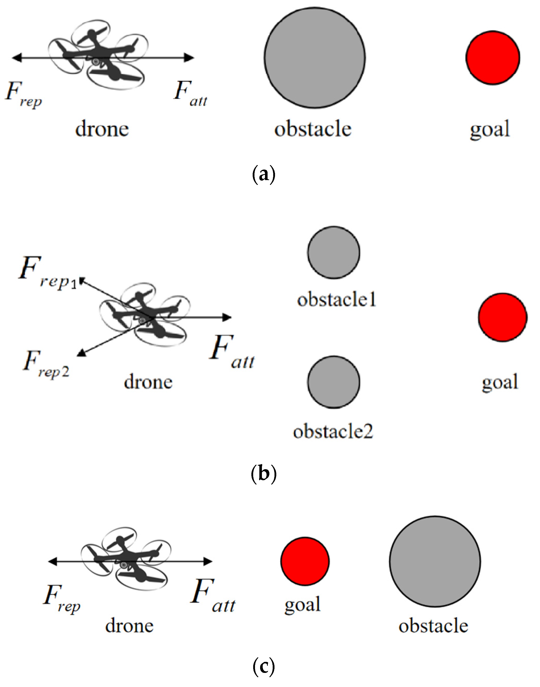
• When the obstacle is directly in front of the target point and the drone is in the same course, and the current drone is subject to gravitational force and repulsive force of the same magnitude and opposite direction, as shown in Figure 12a.
• When the obstacle is on both sides of the drone and the combined direction of the repulsive force is opposite to the direction of the gravitational force and has the same magnitude, as shown in Figure 12b.
• When the obstacle is behind the target point and the repulsive force is much larger than the gravitational force, as shown in Figure 12c.

When the drone is in a local optimum, the situation is divided into two types based on whether there is direct visibility between the drone and the target point. First, as shown in Figure 12a, the obstacle is between the drone and the target point, and it can be found through the 3D LOS visibility detection that the drone cannot reach directly through the obstacle, and it must be affected by unequal external forces, thus breaking the force balance of the drone. Therefore, in this paper, in the case that the drone is caught in the local optimal solution and there is no direct visibility between the drone and the target point, the virtual-target gravitational field is added around the local optimal point to induce the drone to escape, as shown in Figure 13.

When the drone is trapped in a local optimal solution but has direct visibility, the 3D Bresenham’s Line algorithm can be used to test whether a straight line course between the drone and the target is directly reachable. If a direct route is available between the drone and the target point then the current drone is directly connected to the target point location, as shown in Figure 14.

Among them, the 3D Bresenham’s line algorithm plays a key role in driving the local optimal solution and trajectory regression of the drone escape. Bresenham’s line algorithm was previously used in bitmap images to determine the raster of pixels through which the line determined between two points passes. Bresenham’s line algorithm is very effective in 2D grid maps to test for the presence of obstacles between two points, but it is not applicable in 3D stereoscopic space. In this paper, Bresenham’s line algorithm is further extended in three-dimensional space, and step sampling is used to detect whether two points are directly accessible to each other. The implementation steps are given in pseudocode in this article, as follows (Algorithm 3).

Algorithm 3: 3D Bresenham Line

4. Experiment

In this paper, three sets of experiments are conducted for the proposed 3D JPS algorithm using Matlab 2020b (By MathWorks, Inc., Portola Valley, CA, USA) simulation software based on the i5-1135G7 mobile computer (From Lenovo China).

In experiment 1, randomized obstacle distribution and algorithm comparison experiments were conducted for maps of different sizes with different obstacle proportions given the path start and end points. This is used to examine the effectiveness of the 3D JPS algorithm operating under different specification maps.

In experiment 2, a map of the mountain area in the GIS dataset and a map of the city dataset from the Moving AI Lab were selected for the simulation of the 3D JPS algorithm with any-angle path planning and the 3D JPS algorithm with polynomial difference optimization.

In Experiment 3, a 3D JPS algorithm obstacle avoidance test is conducted based on a map of the central London area, using single dynamic threat, linear dynamic threat, and multi-dynamic threats, respectively, as a way to verify the feasibility of the obstacle avoidance strategy proposed in this paper.

The x-axis, y-axis, and z-axis coordinates in the experimental scenes under all designed 3D grid maps in the three sets of experiments are in meters.

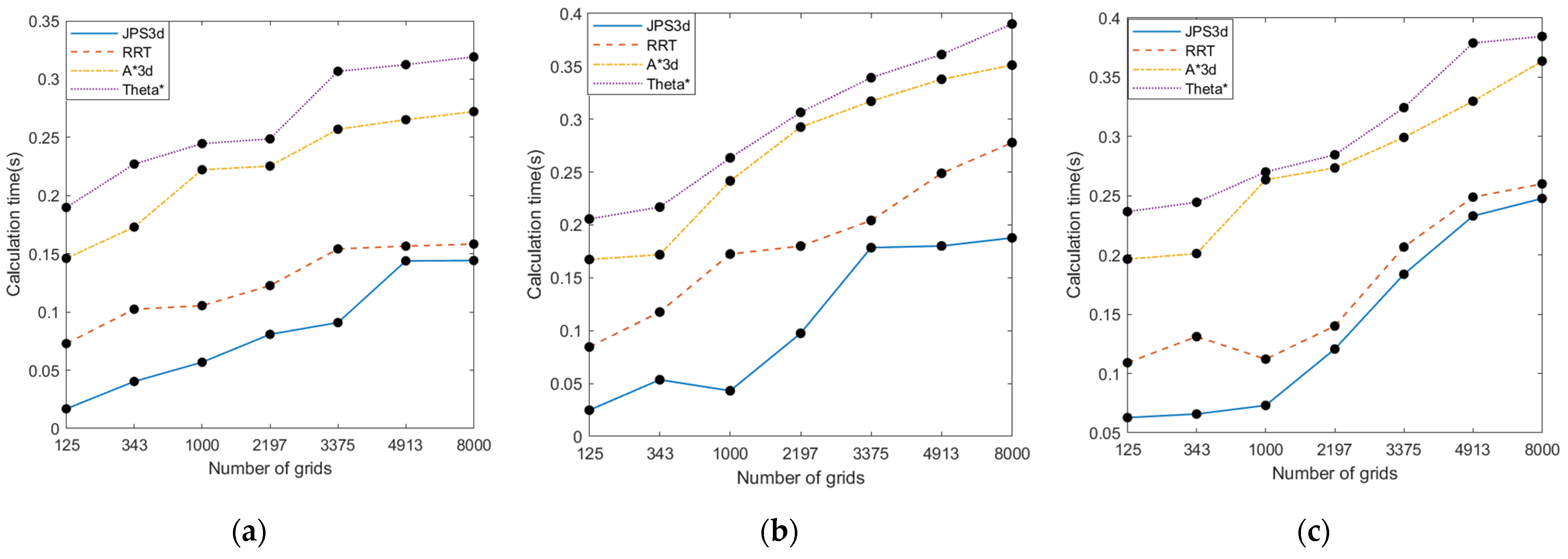
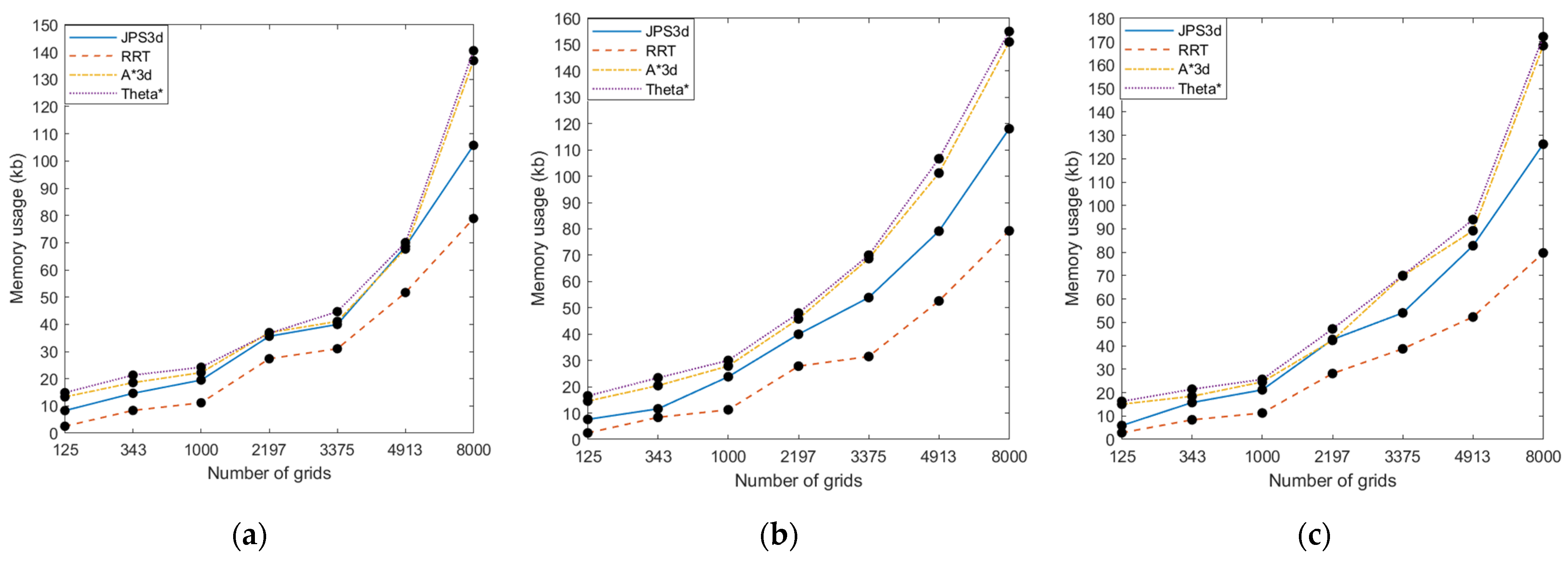
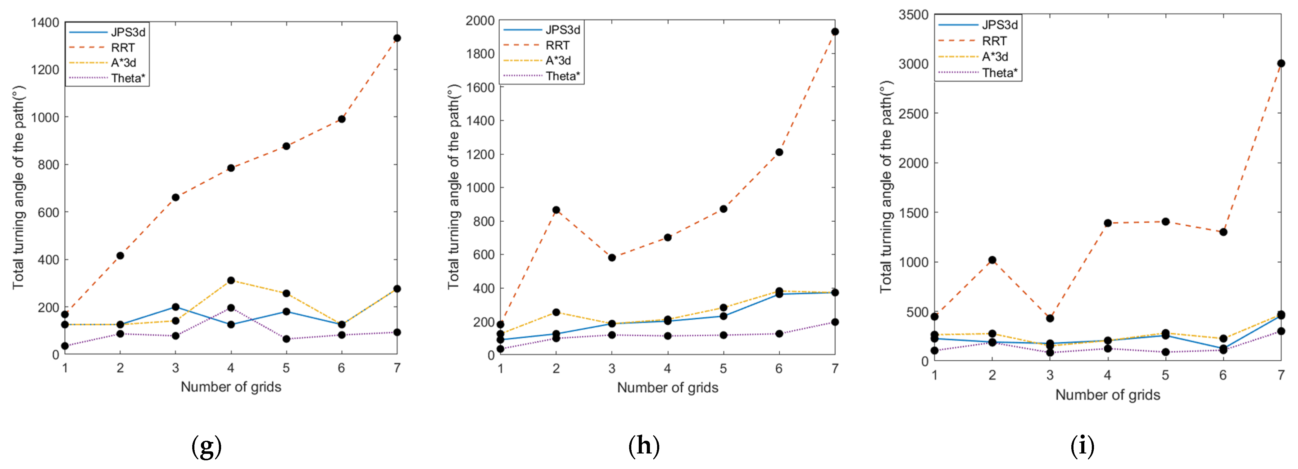
4.1. Randomized-Map Experiment

In this paper, maps consisting of 125 grids, 343 grids, 1000 grids, 2179 grids, 3375 grids, 4913 grids, and 8000 grids are used in the design of the randomness maps, and the percentage of obstacles in each map is 20% to 40%. The computation time, space occupation rate, number of path nodes, path length, and total path-turning angle of the 3D JPS algorithm, 3D A* algorithm, RRT algorithm, and Theta* algorithm are summarized and analyzed, respectively. In the simulation experiments, the Euclidean distance formula is uniformly chosen as the distance calculation of the heuristic function in this paper. The experimental results were taken from the average of 10 experiments. The simulation results are partially shown in Figure 15 below.

As can be seen in Figure 15, the 3D JPS algorithm can complete the global path planning in 3D space with different sizes and different obstacle occupancy of the map. The data of the four algorithms involved in the experimental comparison process are further presented and explained.

In terms of the time complexity of the algorithm, the 3D JPS algorithm had a better performance in the comparison of the four spatial-pathfinding algorithms, as shown in Figure 16. However, it is very obvious that as the number of map grids and the percentage of obstacles increased, all four algorithms used in the experimental process invariably showed an increase in algorithm computation time. In the same map environment, the 3D JPS algorithm had the lowest computation time and the Theta* algorithm had the highest computation time. The 3D JPS algorithm reduced the computation time by 88.45% to 30.18% compared to the 3D A* algorithm and by 34.83% to 4.75% compared to the RRT algorithm. Analyzing the average growth rate of the algorithm’s computation time, we can find that the 3D JPS algorithm will improve the computation time by 0.45% to 1.18% for every 10% increase in the number of grids with the same percentage of obstacles. With the same number of grids in the map, the computation time of the 3D JPS algorithm will be improved by 46.98% to 153.31% for every 10% increase in obstacle percentage. It can be seen that the percentage of the number of obstacles has a large impact on the computation time of the 3D JPS algorithm.

The analysis was performed in terms of the memory usage of the algorithm, as shown in Figure 17. The RRT algorithm had the lowest memory usage among the four algorithms, followed by the 3D JPS algorithm, while the Theta* algorithm had the highest memory usage. The memory usage of the 3D JPS algorithm was 28.72% to 48.32% higher compared to the RRT algorithm and 2.72% to 37.78% lower compared to the A* algorithm. The memory footprint of all four algorithms increased as the map size and obstacle percentage increased. The number of grids was increased by 10% at a time for a map with the same percentage of obstacles. The RRT algorithm had the highest average growth rate of 4.89% in memory usage. The Theta* algorithm had the lowest growth rate of 1.31%. The 3D JPS algorithm had an average growth ratio of 2.26% in the middle region of memory occupation.

From the perspective of the number of path nodes, the length of generated paths, and the total number of path turns, the Theta* algorithm has a definite advantage. The any-angle path planning strategy of the Theta* algorithm causes it to ignore most of the redundant nodes generated by the A* algorithm during the search process, as shown in Figure 18a–c. Also, because the Theta* algorithm is no longer limited by the expansion angle during the search process, it results in a shorter generated path, as shown in Figure 18d–f, and a smaller total path turning angle, as shown in Figure 18g–i. On the contrary, the RRT algorithm is limited by the design of the step size, which leads to an inevitable significant increase in the number of nodes as the map size increases. Additionally, the random-search nature of RRT can lead to too many path-turning angles and poor smoothness. The 3D JPS algorithm was similar to the 3D A* algorithm in terms of the number of path nodes, the total length of the path, and the total turn angle of the path in the comparison experiments of the four algorithms. The 3D JPS algorithm increased the path length by 0.583% to 5.9% and the total path-turning angle by 27% to 98.2% compared to the Theta* algorithm. The 3D JPS algorithm is not optimal in terms of path quality because its search angle is limited by the discretized grid map. There are still redundant turn points in the paths generated by the 3D JPS algorithm that can be optimized, and these unnecessary turn points cause the 3D JPS algorithm to be higher than the Theta* algorithm, which supports any-angle path planning, in terms of path length and total turn angle.

Through the comparative analysis of five sets of metrics for the 3D spatial path-planning algorithm, it can be seen that the 3D JPS algorithm performs better in terms of time complexity and space complexity, but its generated result paths still need further optimization and improvement in terms of length and smoothness.

4.2. 3D JPS Algorithm Trajectory Optimization Experiment Based on Open Dataset

In this paper, we use the maps of London, Boston, and New York City Center from the public database of Moving AI Lab and the mountain areas from the GIS map database to compare the resultant paths of the 3D JPS algorithm, the parent node transfer rule, and the polynomial interpolation optimization, respectively. This is to verify the effectiveness and realism of trajectory optimization based on path generation by the 3D JPS algorithm. In this paper, the path after parent node optimization is abbreviated as PNP-JPS; then, the path after the polynomial-interpolation optimization is abbreviated as OP-PNP-JPS for the convenience of presentation. The experimental results are shown below.

As shown in Figure 19, the optimized 3D JPS algorithm based on the parent node transfer law cuts out a large number of unnecessary turnaround nodes and further reduces the total length of the generated paths. The seventh-order polynomial-interpolation optimization based on the minimum snap again smooths the path to ensure the continuity and smoothness of the position, velocity, acceleration, and jerk of the generated path at each interpolation node, while using the snap as the optimization goal further ensures that the final generated path is the path with the least energy consumption by the drone. In this paper, the experimental results are presented as shown in

Table 1. Map information selected for the dataset.

Map Name	Algorithm Type	Path Length (m)	Total Turning Angle of the Path (°)	Calculation Time (s)	Memory Usage (kb)	Number of Nodes
mountain region 1	JPS3d	156.385	1976.610	9.848	12,678.968	108
	PNP-JPS3d	144.965	421.465	10.029	12,679.540	14
	OP-PNP-JPS3d	144.966	NULL	10.384	12,681.331	501
mountain region 2	JPS3d	125.187	1011.851	12.120	14,137.523	91
	PNP-JPS3d	115.041	183.576	12.302	14,138.243	11
	OP-PNP-JPS3d	115.148	NULL	12.421	14,138.492	495
mountain region 3	JPS3d	137.329	1515.288	8.795	14,991.102	94
	PNP-JPS3d	130.699	732.246	9.035	14,991.821	25
	OP-PNP-JPS3d	130.700	NULL	9.506	14,992.329	507
London	JPS3d	82.332	546.057	5.503	9217.221	16
	PNP-JPS3d	78.036	143.024	5.580	9218.319	10
	OP-PNP-JPS3d	78.038	NULL	5.739	9218.970	477
New York	JPS3d	93.629	1195.529	6.946	9679.211	33
	PNP-JPS3d	87.548	255.291	7.171	9680.490	11
	OP-PNP-JPS3d	87.550	NULL	7.233	9680.992	483
Boston	JPS3d	113.470	520.528	9.603	10,149.380	25
	PNP-JPS3d	107.483	35.567	9.787	10,150.194	4
	OP-PNP-JPS3d	107.284	NULL	9.871	10,150.870	499

.

From Table 1, it can be seen that the optimized path based on the parent node transfer law removes unnecessary redundant turning points from the path generated by the 3D JPS algorithm, making the optimized path length and smoothness better than the original path. The paths optimized based on the parent node transfer law are 4.8% to 8.1% shorter than those obtained by the original 3D JPS algorithm, and the total turning angle of the paths is reduced by 51.6% to 93.2%, with a significant effect on the overall optimization of the paths. In terms of the time and space complexity of the algorithm, the newly added functional modules of the algorithm will inevitably lead to an increase in the running time of the algorithm and an increase in memory usage. The optimized algorithm based on the parent node transfer law increases the computing time by 1.4% to 3.2% and the memory usage by 0.0045% to 0.012% over the original 3D JPS algorithm. In order to ensure the continuity of position, velocity, acceleration, and other information of the final path at each path interruption point, the optimized path based on the parent node transfer law needs to be further optimized by polynomial interpolation. The seventh-order polynomial-interpolation method based on minimum snap used in this paper achieves the optimal smoothness and continuity in the path without affecting the overall computing time and memory consumption of the algorithm as much as possible. As can be seen in Table 1, the paths optimized by the parent node transfer law and polynomial interpolation only increase in computing time by 2.5% to 5.4% and memory usage by 0.0014% to 0.0018% compared to the 3D JPS algorithm.

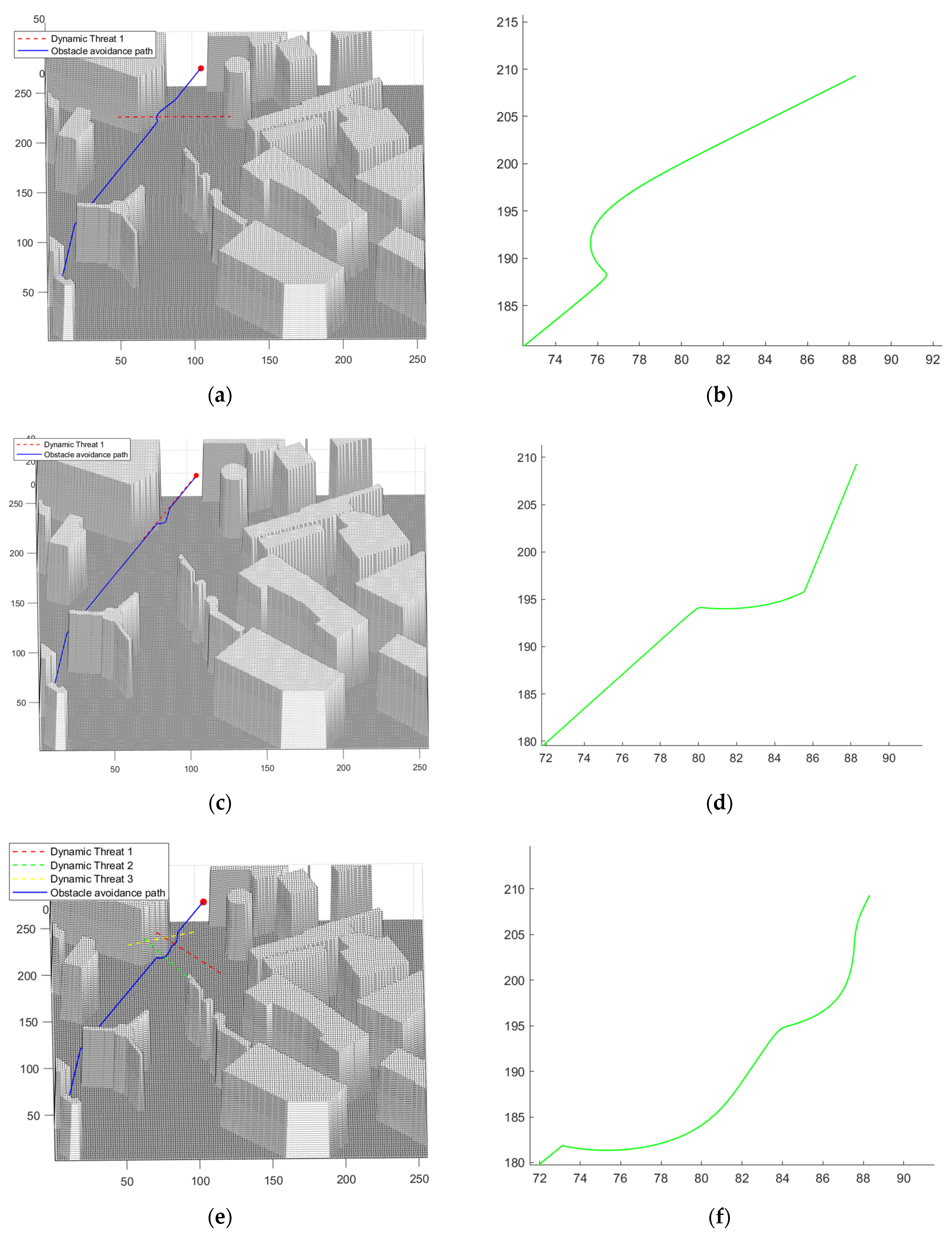
4.3. Dynamic-Threat-Based Drone Obstacle Avoidance Experiments

In this experiment, we simulated and tested a single dynamic threat, a same trajectory inverse threat, and multi-dynamic threats based on the map of some areas of Shanghai City Center in a public dataset. In the design of this experiment, the alert range of the drone was selected based on the mean value of the precise detectable range (20 m) of the forward and side view of the laboratory drone testbed DJI Mavic 2 in a spherical envelope. When the dynamic threat entered the alert range, the artificial potential field method was adopted for dynamic-obstacle avoidance. The repulsive field range generated by the obstacle in the artificial potential field method was set to 5 m, which is the average of the precise measurement range of the DJI Mavic 2 forward and lateral infrared sensors of the drone test platform. When the distance between the drone and the obstacle was less than or equal to 5 m, there was a repulsive effect on the drone. The experimental results are shown in Figure 20.

First, during the single dynamic threat test, the intruder was at the same height as the drone and performed a collision conflict with an oblique lateral insertion, as shown in Figure 19a. The artificial-potential-field method started to execute at a distance of 20 m from the drone detecting the dynamic threat and changed its path at a straight line distance of 5 m from the obstacle by the real-time-changing repulsion, where the minimum distance between the drone and the dynamic threat was 4.38 m. The obstacle avoidance path generated by the artificial-potential-field method itself was a smooth path, but the sudden switch between the 3D JPS algorithm and the artificial-potential-field method in the pathfinding process led to the possibility of a large turn in the path, as shown in Figure 19b. Second, in the same-trajectory reverse-conflict experiment, because the dynamic threat was between the drone and the target point and moved along the drone trajectory in the reverse direction, the gravitational force of the target point by the drone was opposite to the direction of the repulsive force given by the dynamic obstacle, and it was very easy for it to fall into the local optimal solution. In the improved artificial potential field algorithm, the virtual target gravitational field and the 3D Bresenham’s line algorithm can contribute to the successful escape of the drone, but the final generated path still appears unsmooth due to the characteristics of the Bresenham’s line as a straight line segment, as shown in Figure 19d The minimum distance between the drone and the dynamic threat was 3.94 m. Finally, in this paper, we conducted experiments on the improved artificial-potential-field method based on the multi-dynamic threats scenario, as shown in Figure 19e. From the experimental results, the three dynamic intrusions were detected by the drone at (195.2040,70.0319,30), (206.7423,77.8219,30), and (95.8219,205.7992,30), respectively, while the minimum distances between the drone and the dynamic threats were 4.21 m, 4.46 m, and 3.35 m. From the path generation results, the improved artificial-potential-field method met the dynamic-threat avoidance requirements for a near-ground search drone, but further optimization is still needed for generating paths.

5. Simulation

For drones performing near-ground search and rescue, the complexity of the environment, the high number of obstacles, and the presence of dynamic threats all pose significant challenges to the path planning of drones. Based on the above problems, the main work of this paper lies in three aspects, which are summarized as follows.

• For the static obstacles in the drone’s working environment, this paper extended the JPS algorithm in three dimensions to guide the drone to perform the mission in the 3D space. The algorithm comparison experiments showed that the 3D JPS algorithm had good expressiveness in terms of time complexity and space complexity. The 3D JPS algorithm reduced the computation time by 88.45% to 30.18% compared to the 3D A* algorithm and by 34.83% to 4.75% compared to the RRT algorithm. The 3D JPS algorithm met the demand for high efficiency in drone search-and-rescue missions. However, it was also found in the comparison experiments that the quality of the final generated paths of the 3D JPS algorithm did not reach the optimum. The 3D JPS algorithm increased the path length by 0.583% to 5.9% and the total path-turning angle by 27% to 98.2% compared to the Theta* algorithm.
• In this paper, the parent node transfer law was used to optimize the generation path for the 3D JPS algorithm. The any-angle path planning of the 3D JPS algorithm was achieved by changing the parent–child node relationship chain among the path nodes to eliminate redundant turning points. Second, this paper introduced seventh-order polynomial-interpolation optimization based on minimum snap to further improve the smoothness and continuity of the path generated by the 3D JPS algorithm. As can be seen from experiment 2, the paths optimized based on the parent node transfer law were 4.8% to 8.1% shorter than the paths obtained by the 3D JPS algorithm, and the total turning angle of the paths was reduced by 51.6% to 93.2%, and the overall optimization effect of the paths is obvious. At the same time, the time complexity as well as the space complexity of the algorithm increased due to the parent node transfer law and polynomial-interpolation optimization, and the computing time increased by 2.5% to 5.4% and the memory usage increased by 0.0014% to 0.0018% compared to the 3D JPS algorithm.
• Finally, this paper used an improved artificial-potential-field-based obstacle avoidance strategy to avoid the dynamic threats that may occur in drone low-level flight operations. Firstly, this paper improved the artificial-potential-field method to address the problem of falling into local optimum, by adding a virtual-target gravitational field and the three-dimensional Bresenham’s line algorithm to induce the drone to achieve local-optimum escape. Secondly, the 3D JPS algorithm combined with an improved artificial-potential-field method was used to avoid obstacles for dynamic threats that come within the alert range. Experiment 3 showed that the dynamic-obstacle-avoidance strategy based on the improved artificial-potential-field method successfully accomplished the obstacle avoidance task in the cases of a single intruder, a reverse intruder with the same trajectory, and multiple intruders. However, the conversion of the 3D JPS algorithm to the artificial-potential-field method and the characteristics of the 3D Bresenham’s line algorithm still led to the problem of unsmooth and excessive cornering in the final result path.

The next work in this paper needs to further optimize the dynamic-obstacle-avoidance strategy of the 3D JPS algorithm and further reduce the computation time of the 3D JPS algorithm in order to improve the quality of the algorithm-generated path and the computation efficiency of the algorithm.

References

1. Patle, B.; Pandey, A.; Parhi, D.; Jagadeesh, A. A review: On path planning strategies for navigation of mobile robot. Def. Technol. 2019, 15, 582–606. [Google Scholar] [CrossRef]
2. Kontitsis, M.; Valavanis, K.P.; Tsourveloudis, N. A UAV vision system for airborne surveillance. In Proceedings of the IEEE International Conference on Robotics and Automation (ICRA’04), New Orleans, LA, USA, 26 April–1 May 2004; pp. 77–83. [Google Scholar]
3. Dileep, M.; Navaneeth, A.; Ullagaddi, S.; Danti, A. A study and analysis on various types of agricultural drones and its applications. In Proceedings of the 2020 Fifth International Conference on Research in Computational Intelligence and Communication Networks (ICRCICN), Bangalore, India, 26–27 November 2020; pp. 181–185. [Google Scholar]
4. Dorling, K.; Heinrichs, J.; Messier, G.G.; Magierowski, S. Vehicle routing problems for drone delivery. IEEE Trans. Syst. Man Cybern. Syst. 2016, 47, 70–85. [Google Scholar] [CrossRef] [Green Version]
5. Vashisth, A.; Batth, R.S.; Ward, R. Existing Path Planning Techniques in Unmanned Aerial Vehicles (UAVs): A Systematic Review. In Proceedings of the 2021 International Conference on Computational Intelligence and Knowledge Economy (ICCIKE), Dubai, United Arab Emirates, 17–18 March 2021; pp. 366–372. [Google Scholar]
6. Yang, L.; Qi, J.; Xiao, J.; Yong, X. A literature review of UAV 3D path planning. In Proceedings of the Proceeding of the 11th World Congress on Intelligent Control and Automation, Shenyang, Chain, 29 June–4 July 2014; pp. 2376–2381. [Google Scholar]
7. Rivera, A.; Villalobos, A.; Monje, J.C.N.; Mariñas, J.A.G.; Oppus, C.M. Post-disaster rescue facility: Human detection and geolocation using aerial drones. In Proceedings of the 2016 IEEE Region 10 Conference (TENCON), Singapore, 22–25 November 2016; pp. 384–386. [Google Scholar]
8. Cangan, B.G.; Heintzman, L.; Hashimoto, A.; Abaid, N.; Williams, R.K. Anticipatory human-robot path planning for search and rescue. arxiv 2020, 2009, 03976. [Google Scholar] [CrossRef]
9. Mishra, B.; Garg, D.; Narang, P.; Mishra, V. Drone-surveillance for search and rescue in natural disaster. Comput. Commun. 2020, 156, 1–10. [Google Scholar] [CrossRef]
10. Zhang, N.; Zhang, M.; Low, K.H. 3D path planning and real-time collision resolution of multirotor drone operations in complex urban low-altitude airspace. Transp. Res. Part C Emerg. Technol. 2021, 129, 103123. [Google Scholar] [CrossRef]
11. McRae, J.N.; Gay, C.J.; Nielsen, B.M.; Hunt, A.P. Using an unmanned aircraft system (drone) to conduct a complex high altitude search and rescue operation: A case study. Wilderness Environ. Med. 2019, 30, 287–290. [Google Scholar] [CrossRef] [Green Version]
12. Shahid, N.; Abrar, M.; Ajmal, U.; Masroor, R.; Amjad, S.; Jeelani, M. Path planning in unmanned aerial vehicles: An optimistic overview. Int. J. Commun. Syst. 2022, 35, e5090. [Google Scholar] [CrossRef]
13. Xiaomeng, Z.; Yongjiang, H.; Wenguang, L. Multi-UAV fire fighting mission planning based on improved artificial bee colony algorithm. J. Chin. Inert. Technol. 2020, 28, 528–536. [Google Scholar]
14. Dong, S. Application research of quadrotor UAV motion planning system based on heuristic search and minimum-snap trajectory optimization. In Proceedings of the 2021 IEEE 5th Advanced Information Technology, Electronic and Automation Control Conference (IAEAC), Chongqing, China, 12–14 March 2021; pp. 2270–2274. [Google Scholar]
15. Chen, H.; Lu, P.; Xiao, C. Dynamic obstacle avoidance for UAVs using a fast trajectory planning approach. In Proceedings of the 2019 IEEE International Conference on Robotics and Biomimetics (ROBIO), Dali, China, 6–8 December 2019; pp. 1459–1464. [Google Scholar]
16. Budiyanto, A.; Cahyadi, A.; Adji, T.B.; Wahyunggoro, O. UAV obstacle avoidance using potential field under dynamic environment. In Proceedings of the 2015 International Conference on Control, Electronics, Renewable Energy and Communications (ICCEREC), Bandung, Indonesia, 27–29 August 2015; pp. 187–192. [Google Scholar]
17. Jianmeng, H.; Yuxiong, W.; Xiezhao, L. Smooth JPS path planning and trajectory optimization method of mobile robot. Nongye Jixie Xuebao/Trans. Chin. Soc. Agric. Mach. 2021, 52, 21–29+121. [Google Scholar]
18. Zha, T.; Li, Y.; Sun, L. A Local Planning Method Based on Minimum Snap Trajectory Generation and Traversable Region for Inspection of Airport Roads. In Proceedings of the 2021 5th International Conference on Automation, Control and Robots (ICACR), Nanning, China, 25–27 September 2021; pp. 38–42. [Google Scholar]
19. Dongcheng, L.; Jiyang, D. Research on Multi-UAV Path Planning and Obstacle Avoidance Based on Improved Artificial Potential Field Method. In Proceedings of the 2020 3rd International Conference on Mechatronics, Robotics and Automation (ICMRA), Shanghai, China, 16–18 October 2020; pp. 84–88. [Google Scholar]
20. Chunfang, X.; Haibin, D.; Fang, L. Chaotic artificial bee colony approach to Uninhabited Combat Air Vehicle (UCAV) path planning. Int. J. Intell. Comp. Cybern. 2010, 14, 535–541. [Google Scholar]
21. Chen, X.; Zhao, M.; Yin, L. Dynamic path planning of the UAV avoiding static and moving obstacles. J. Intell. Robot. Syst. 2020, 99, 909–931. [Google Scholar] [CrossRef]
22. Hrabar, S. 3D path planning and stereo-based obstacle avoidance for rotorcraft UAVs. In Proceedings of the 2008 IEEE/RSJ International Conference on Intelligent Robots and Systems, Nice, France, 22–26 September 2008; pp. 807–814. [Google Scholar]
23. Traish, J.; Tulip, J.; Moore, W. Optimization using boundary lookup jump point search. IEEE Trans. Comput. Intell. AI Games 2015, 8, 268–277. [Google Scholar] [CrossRef]
24. Wei, Y.; Zhu, D.; Chu, Z. Underwater dynamic target tracking of autonomous underwater vehicle based on MPC algorithm. In Proceedings of the 2018 IEEE 8th International Conference on Underwater System Technology: Theory and Applications (USYS), Wuhan, China, 1–3 December 2018; pp. 1–5. [Google Scholar]
25. Kuriki, Y.; Namerikawa, T. Formation control with collision avoidance for a multi-UAV system using decentralized MPC and consensus-based control. SICE J. Control. Meas. Syst. Integr. 2015, 8, 285–294. [Google Scholar] [CrossRef]
26. Yu-Geng, X.; De-Wei, L.; Shu, L. Model predictive control—Status and challenges. Acta Autom. Sin. 2013, 39, 222–236. [Google Scholar]
27. dos Santos, R.R.; Steffen, V.; Saramago, S.d.F. Robot path planning in a constrained workspace by using optimal control techniques. Multibody Syst. Dyn. 2008, 19, 159–177. [Google Scholar] [CrossRef]
28. Lindqvist, B.; Mansouri, S.S.; Agha-mohammadi, A.-A.; Nikolakopoulos, G. Nonlinear MPC for collision avoidance and control of UAVs with dynamic obstacles. IEEE Robot. Autom. Lett. 2020, 5, 6001–6008. [Google Scholar] [CrossRef]
29. Kim, J.-C.; Pae, D.-S.; Lim, M.-T. Obstacle avoidance path planning based on output constrained model predictive control. Int. J. Control. Autom. Syst. 2019, 17, 2850–2861. [Google Scholar] [CrossRef]
30. Khatib, O. Real-time obstacle avoidance for manipulators and mobile robots. In Autonomous Robot Vehicles; Springer: Berlin/Heidelberg, Germany, 1986; pp. 396–404. [Google Scholar]
31. Kumar, P.B.; Rawat, H.; Parhi, D.R. Path planning of humanoids based on artificial potential field method in unknown environments. Expert Syst. 2019, 36, e12360. [Google Scholar] [CrossRef]
32. Li, Y.; Tian, B.; Yang, Y.; Li, C. Path planning of robot based on artificial potential field method. In Proceedings of the 2022 IEEE 6th Information Technology and Mechatronics Engineering Conference (ITOEC), Chongqing, China, 4–6 March 2022; pp. 91–94. [Google Scholar]
33. Wang, H.; Hao, C.; Zhang, P.; Zhang, M.; Yin, P.; Zhang, Y. Path planning of mobile robots based on A* algorithm and artificial potential field algorithm. China Mech. Eng. 2019, 30, 2489. [Google Scholar]
34. Harabor, D.; Grastien, A. Online graph pruning for pathfinding on grid maps. In Proceedings of the AAAI Conference on Artificial Intelligence, San Francisco, CA, USA, 7–11 August 2011; pp. 1114–1119. [Google Scholar]
35. Jia, J.; Pan, J.-S.; Xu, H.-R.; Wang, C.; Meng, Z.-Y. An Improved JPS Algorithm in Symmetric Graph. In Proceedings of the 2015 Third International Conference on Robot, Vision and Signal Processing (RVSP), Kaohsiung, Taiwan, 18–20 November 2015; pp. 208–211. [Google Scholar]
36. Luo, Y.; Lu, J.; Qin, Q.; Liu, Y. Improved JPS Path Optimization for Mobile Robots Based on Angle-Propagation Theta* Algorithm. Algorithms 2022, 15, 198. [Google Scholar] [CrossRef]
37. Zhou, K.; Yu, L.; Long, Z.; Mo, S. Local path planning of driverless car navigation based on jump point search method under urban environment. Future Internet 2017, 9, 51. [Google Scholar] [CrossRef] [Green Version]
38. Mellinger, D.; Kumar, V. Minimum snap trajectory generation and control for quadrotors. In Proceedings of the 2011 IEEE international conference on robotics and automation, Shanghai, China, 9–13 May 2011; pp. 2520–2525. [Google Scholar]
Figure 1. No-Fly Zone in Montreal from DJI.
Applsci 12 07333 g001
Figure 2. Search-angle limitation of JPS algorithm. (a) Limitation of extension angle of JPS algorithm in 2D structure, (b) Limitation of extension angle of JPS algorithm in 3D structure.
Applsci 12 07333 g002
Figure 3. The working framework of this article.
Applsci 12 07333 g003
Figure 4. Comparison between A* algorithm and JPS algorithm for accessing nodes in the search process. (a) A* algorithm path-planning process. (b) JPS algorithm path-planning process.
Applsci 12 07333 g004
Figure 5. JPS algorithm’s neighbor-pruning rule and forced-neighbor judgment method. (a) Neighbor pruning in the linear extension state. (b) Neighbor pruning in the diagonal expansion state. (c) Forced neighbors in the linear extension state. (d) Forced neighbors in diagonally extended states.
Applsci 12 07333 g005
Figure 6. Minimum set of JPS algorithm in 2D and 3D space. (a) 2D JPS path search minimum set. (b) 3D JPS path search minimum set.
Applsci 12 07333 g006
Figure 7. Three-dimensional JPS algorithm neighbor-pruning law. (a) Pruning rule under the linear extension direction in the same plane. The expansion direction of the 3D JPS algorithm is restricted to the original expansion direction in the unique plane. (b) Pruning rule under the diagonal extension direction of the same plane. The expansion direction of the 3D JPS algorithm is restricted to the original expansion direction in the unique plane as well as above and to the right of the current grid. (c) Pruning rules under the diagonal expansion direction of the body. The extension direction of the 3D JPS algorithm will involve two planes. Where the green arrow indicates the expansion direction of the parent node from the lower layer to the current node, the red arrow indicates the expansion direction of the middle layer, and the blue arrow indicates the expansion direction from the current node to the upper layer.
Applsci 12 07333 g007
Figure 8. Three-dimensional JPS algorithm extension method. (a) Same-plane linear extension. (b) Same-plane diagonal extension. (c) Body diagonal extension.
Applsci 12 07333 g008
Figure 9. Trajectory optimization framework.
Applsci 12 07333 g009
Figure 10. JPS algorithm parent–child node relationship chain.
Applsci 12 07333 g010
Figure 11. Comparison between the actual spatial shortest path and the path obtained by JPS algorithm. (a) Comparison of the actual spatial shortest path and the path obtained by the 2D-JPS algorithm. (b) Comparison of the actual spatial shortest path and the path obtained by the 3D-JPS algorithm.
Applsci 12 07333 g011
Figure 12. Artificial-potential-field method falls into the local-optimum case. (a) The obstacle is directly in front of the target point and on the same course as the drone. (b) Obstacles are on both sides of the drone. (c) The obstacle is behind the target point and on the same course as the drone.
Applsci 12 07333 g012
Figure 13. Escape local optimal solution using virtual-target gravitational field. (a) Traditional artificial-potential-field method. (b) Improved artificial-potential-field method.
Applsci 12 07333 g013
Figure 14. Escaping Local Optimal Solutions Using the 3D Bresenham’s Line Algorithm. (a) Traditional artificial-potential-field method. (b) Improved artificial-potential-field method. (c) Traditional artificial-potential-field method. (d) Improved artificial-potential-field method.
Applsci 12 07333 g014
Figure 15. Experimental comparison of algorithms based on randomness maps. (a) Obstacles accounted for 20%. (b) Obstacles accounted for 30%. (c) Obstacles accounted for 40%. (d) Obstacles accounted for 20%. (e) Obstacles accounted for 30%. (f) Obstacles accounted for 40%. (g) Obstacles accounted for 20%. (h) Obstacles accounted for 30%. (i) Obstacles accounted for 40%. (j) Obstacles accounted for 20%. (k) Obstacles accounted for 30%. (l) Obstacles accounted for 40%.
Applsci 12 07333 g015aApplsci 12 07333 g015b
Figure 16. Experimental comparison of algorithms based on randomness maps. (a) Obstacles accounted for 20%. (b) Obstacles accounted for 30%. (c) Obstacles accounted for 40%.
Applsci 12 07333 g016
Figure 17. Algorithm memory usage comparison. (a) Obstacles accounted for 20%. (b) Obstacles accounted for 30%. (c) Obstacles accounted for 40%.
Applsci 12 07333 g017
Figure 18. Comparison of the number of path nodes, total path length, and total path-turning angle. (a) Comparison of the number of path nodes based on 20% obstacle-occupied maps. (b) Comparison of the number of path nodes based on 30% obstacle-occupied maps. (c) Comparison of the number of path nodes based on 40% obstacle-occupied maps. (d) Total path length based on 20% obstacle-occupied maps. (e) Total path length based on 30% obstacle-occupied maps. (f) Total path length based on 40% obstacle-occupied maps. (g) Total turning angle of the path based on 20% obstacle-occupied maps. (h) Total turning angle of the path based on 30% obstacle-occupied maps. (i) Total turning angle of the path based on 40% obstacle-occupied maps.
Applsci 12 07333 g018aApplsci 12 07333 g018b
Figure 19. Three-dimensional JPS algorithm generates paths and its trajectory optimization path comparison experiment. (a) Map of the mountain region 1. (b) Map of London. (c) Map of the mountain region 2. (d) Map of New York. (e) Map of the mountain region 3. (f) Map of Boston.
Applsci 12 07333 g019
Figure 20. Drone dynamic-obstacle avoidance experiment based on artificial potential field method. (a) Single-dynamic-threat avoidance. (b) Obstacle avoidance path segments under single dynamic threat based on the artificial potential field approach. (c) Same trajectory reverse dynamic threat avoidance. (d) Obstacle avoidance path segments under inverse dynamic threat of the same trajectory based on the artificial-potential-field method. (e) Multi-dynamic threats avoidance. (f) Artificial potential field based approach for obstacle avoidance path segments under multiple dynamic threats.
Applsci 12 07333 g020