The Parameter Design of Nonlinear Energy Sink Installed on the Jacket Pipe by Using the Nonlinear Dynamical Theory

Abstract

The aim of this paper is to investigate the vibration suppression effect of a nonlinear energy sink (NES) on the wind-vortex-induced vibration of deep-water jacket pipes. Based on nonlinear dynamical theories, the coupled dynamic equation of a deep-water jacket pipe with NES was established, and the nonlinear response characteristics and motion stability of the system were studied by using the multi-scale mixed harmonic balance method and Routh–Hurwitz criterion. The paper also analyzed the influence of the nonlinear stiffness and damping parameters of an NES on the dynamic response of the pipe. It is concluded that when the nonlinear stiffness of an NES increases to a certain extent, the motion response of the pipe appeared as a saddle-node and Hopf bifurcation, and the vibration amplitude of the pipe is greatly suppressed. For a system with nonlinear motion, NES damping mainly affects the range of the unstable region. For the system without nonlinear motion, the increases in NES damping will reduce the amplitude near the resonance region. Selecting proper parameters of an NES nonlinear stiffness and damping can effectively suppress the vortex-induced vibration of pipes.

1. Introduction

With the deeper working water depth, larger structure dimension, smaller structural stiffness and lower natural frequency of the jacket platform, the structure is more prone to resonance. This will affect the safe production and service life of the jacket structure and may even lead to fatigue failure [1,2]. Therefore, it is important to reasonably suppress wind-vortex-induced vibration.

At present, the vortex-induced vibration control of marine engineering structures mainly includes four methods [3]: passive control, active control, semi-active and hybrid control. Active control and semi-active control may require external energy equipment for energy supply, sensors and other devices. Compared with passive control, active control seems more complicated. A nonlinear energy sink (NES) is a type of passive vibration absorber that was originally developed from the concept of a dynamic vibration absorber proposed by Frahm [4]. Vakakis [5] first proposed the concept of an NES with nonlinear stiffness. Compared with a traditional linear vibration absorber, it could effectively absorb the vibration energy of the main structure in a wide frequency range and further dissipate the energy by using damping elements. Georgiades et al. [6] used an NES in a linear beam to reduce vibrations. The results show that an NES dissipates 87% of the energy when specific parameters are selected. Ahmadabadi et al. [7] added an NES to a cantilever beam to reduce vibration. The results show that 89% energy dissipation can be achieved through parameter optimization. Zhou et al. [8] added an NES to a cantilever pipe with internal fluid and analyzed the influence of different positions and NES parameters on the vibration suppression effect. Zhang et al. [9] studied the vibration suppression of a beam with an NES and analyzed the influence of NES parameters.

Some scholars used an NES to suppress the vortex-induced vibration of slender structures, which achieved a good vibration suppression effect. Dai et al. [10] simulated the vortex-induced vibration response of a rigid pipe under wind loads by using the wake oscillator model, and the results show that the structural vibration is minimized through adjustment of the mass ratio of an NES. Chen et al. [11] used CFD to analyze the vortex-induced vibration of pipes with an NES and calculated the response of pipes considering a two-degrees-of-freedom system. The results show that the vibration of steel pipes is significantly reduced after adding an NES. Blanchard et al. [12] studied a rotating NES inside the pipe in which the displacement of the NES was not limited, and obvious vibration reduction effects were obtained.

Current research shows that when an NES is used to suppress the vortex-induced vibration of elastic structures, the response of structures is complex due to the nonlinearity of an NES, and even amplitude jumps and unstable motion will occur for certain parameters. In addition, the NES’s parameters have a significant influence on the motion forms and vibration suppression effects [13]. In this paper, an NES is used to suppress the wind-vortex-induced vibration of a deep-water jacket pipe, and the nonlinear response of the system was analyzed. The design parameter of an NES was suggested according to the results of the nonlinear analysis.

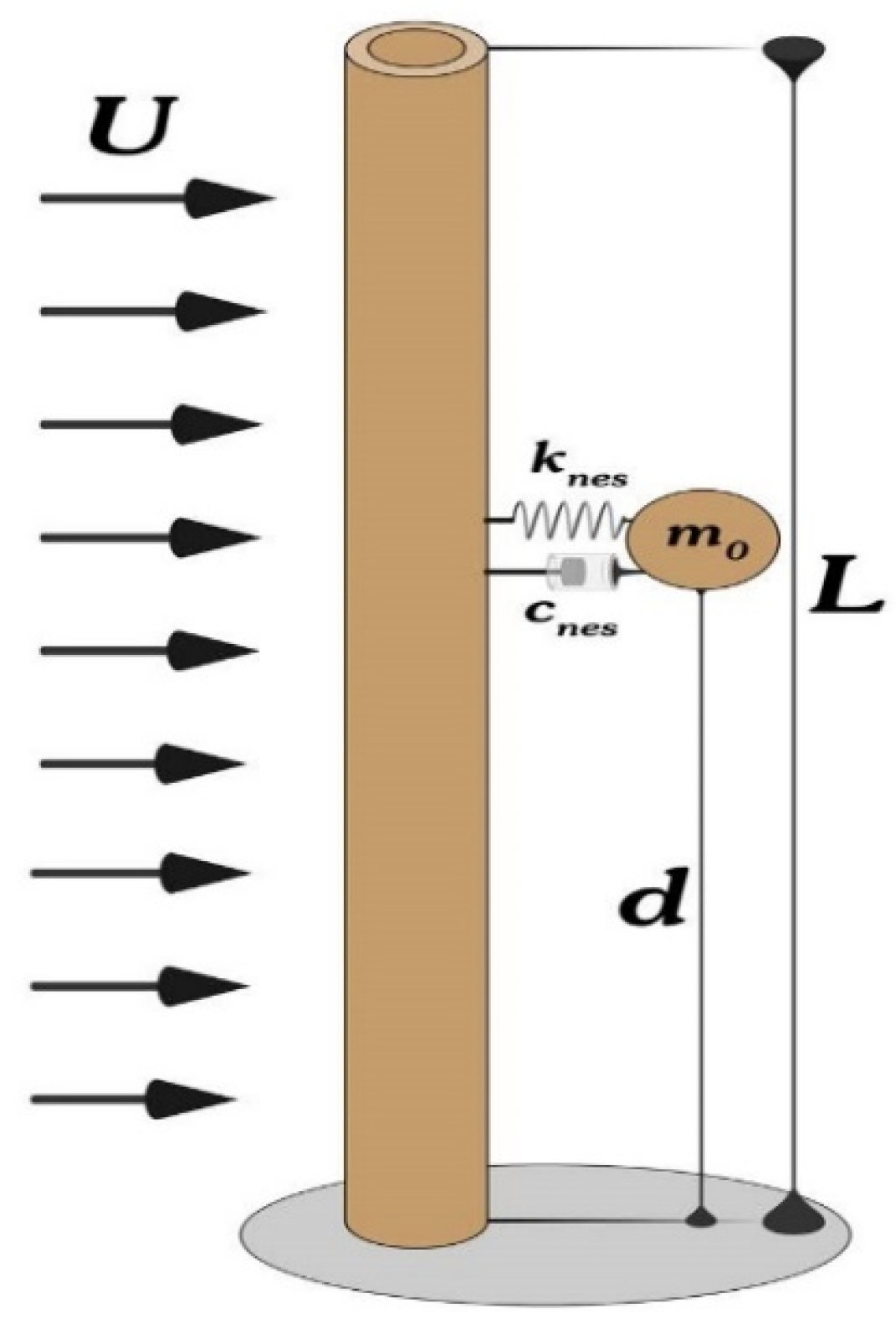
2. Establishment of Pipe-NES Coupling Dynamic Model

An NES is composed of a mass oscillator, a cubic stiffness spring and damping, which dissipate the energy transmitted by the main system and then reduce the vibration of the main system. Due to the cubic stiffness spring, an NES system has a variable natural frequency, which can achieve significant vibration suppression effects [14]. The first mode of the deep-water jacket pipe is more likely to cause wind-vortex-induced vibration. The pipe is treated as a single-degree-of-freedom mass-spring-damping system [15] (the main system). The system of the pipe with an NES (the subsystem) is shown in Figure 1.

Considering an NES, the transverse vibration of a pipe induced by the wind-vortex force is written as follows [16]:

$$\{\begin{array}{c}{m}_1{\ddot{x}}_1+c_1{\dot{x}}_1+k_1{x}_1+c_{nes}({\dot{x}}_1-{\dot{x}}_2)+k_{nes}{(x_1-x_2)}^3=f_L\\ m_{nes}{\ddot{x}}_2+c_{nes}({\dot{x}}_2-{\dot{x}}_1)+k_{nes}{(x_2-x_1)}^3=0\end{array}$$

(1)

where $m_1$ is the mass of the pipe and $m_{nes}$ is the mass of the NES. $c_1$ is the damping of the pipe, and $c_{nes}$ is the damping of the NES. $k_1$ is the structural stiffness of the pipe, and $k_{nes}$ is the cubic stiffness of the NES. $x_1$, ${\dot{x}}_1$, ${\ddot{x}}_1$ are the transverse displacement, velocity and acceleration of the main system (pipe), respectively. $x_2$, ${\dot{x}}_2$, ${\ddot{x}}_2$ are the displacement, velocity and acceleration of the subsystem (NES) in the direction of wind force, respectively.

The wind-vortex-induced force on the pipe is treated as the harmonic load [17], as follows:

$$f_L=\frac{1}{2}{C}_L\rho U^{2}D\cos (\mathrm{\Omega }t)=F_L\cos (\mathrm{\Omega }t)$$

(2)

where $\mathrm{\Omega }$ is the vortex shedding frequency. To simplify the derivation process, Equation (1) is replaced by the following variables:

$${\xi }_1=\frac{c_1}{m_1},{\xi }_2=\frac{c_{nes}}{m_1},{\omega }^{{}_2}=\frac{k_1}{m_1},k=\frac{k_{nes}}{m_1},{\rho }_2=\frac{m_{nes}}{m_1},F=\frac{F_L}{m_1},z=x_2-x_1$$

where z is the relative displacement of the pipe and NES. The mass of an NES is smaller than that of the pipe. To develop an approximated solution of the equation by using the multi-scale mixed harmonic balance method, the small value parameter $\epsilon$ is introduced to rescale some variables. The motion equation after replacing the variables is:

$$\{\begin{array}{c}{\ddot{x}}_1+\epsilon {\xi }_1{\dot{x}}_1+{\omega }^2{x}_1-\epsilon {\xi }_2\dot{z}-\epsilon \kappa z^3=\epsilon F\cos (\mathrm{\Omega }t)\\ \epsilon {\rho }_2(\ddot{z}+{\ddot{x}}_1)+\epsilon {\xi }_2\dot{z}+\epsilon \kappa z^3=0\end{array}$$

(3)

where $\dot{z}$ is the derivative of z; $\ddot{z}$ is the derivative of $\dot{z}$. The dot represents the derivative of the corresponding parameter.

3. Approximate Solution Based on the Multi-Scale Mixed Harmonic Balance Method

Some scholars have used the complex variable averaging method [18,19], harmonic balance method [20] and multi-scale mixed harmonic balance method [21] to approximately solve motion equations with NES. The multi-scale mixed harmonic balance method does not need to replace the complex variables, which makes the physical meaning of the parameters clearer. Moreover, Yaru et al. [22] investigated a novel method of dynamic force reconstruction based on ANN and BPF and verified it by a numerical example of a cantilever beam. A novel dynamic reliability-based topology optimization (DRBTO) strategy was investigated by Lei et al. [23] for time-variant mechanical systems with overall consideration of material dispersion and loading deviation effects. Lei et al. [24] developed a novel convexity-oriented time-dependent reliability-based topology optimization (CTRBTO) scheme to overcome the current difficulties caused by uncertainties in the DRTO implementation, such as the time-varying reliability evaluation and the design sensitivity derivation. In this work, the multi-scale mixed harmonic balance method is used to solve Equation (3).

3.1. Approximate Analytical Solutions of the Nonlinear Equations

The factor $\sigma$ is introduced to represent the difference between the external excitation frequency and the natural frequency of the pipe, namely, $\mathrm{\Omega }=\omega +\epsilon \sigma$, where $\epsilon$ is a small parameter. Considering the time scale $t_0=t$, $t_1=\epsilon t$, the analytical solution of Equation (3) is set as:

$$\{\begin{array}{c}{x}_1=x_{11}(t_0,t_1)+\epsilon x_{12}(t_0,t_1)\\ z=z_{11}(t_0,t_1)+\epsilon z_{12}(t_0,t_1)\end{array}$$

(4)

We can substitute Equation (4) into Equation (3). According to the coefficients of $\epsilon$ with the same order of two sides of the equation being equal, the following equations are obtained:

$$D_0{}^2{x}_{11}+{\omega }^2{x}_{11}=0$$

(5)

$$D_0{}^2{x}_{12}+{\omega }^2{x}_{12}=\kappa z_{11}{}^3+{\xi }_2{D}_0{z}_{11}-{\xi }_1{D}_0{x}_{11}-2D_0{D}_1{x}_{11}+F\cos (\mathrm{\Omega }t)$$

(6)

$${\rho }_2{D}_0{}^2{x}_{11}+{\rho }_2{D}_0{}^2{z}_{11}+\kappa z_{11}{}^3+{\xi }_2{D}_0{z}_{11}=0$$

(7)

$$D_1{}^2{x}_{11}+2D_0{D}_1{x}_{12}+{\xi }_1{D}_0{x}_{12}+{\xi }_1{D}_1{x}_{11}-{\xi }_2{D}_0{z}_{12}-{\xi }_2{D}_1{z}_{11}-3\kappa z_{11}{}^2{z}_{12}=0$$

(8)

$$\begin{array}{l}{\rho }_2{D}_0{}^2{x}_{12}+{\rho }_2{D}_0{}^2{z}_{12}+2{\rho }_2{D}_0{D}_1{x}_{12}+2{\rho }_2{D}_0{D}_1{z}_{11}\\ +{\xi }_2{D}_1{z}_{11}+{\xi }_2{D}_0{z}_{12}+3\kappa z_{11}{}^2{z}_{12}=0\end{array}$$

(9)

where $D_i(i=1,2)$ is the differential operator [21]. Higher-order terms, such as 3Ω and 5Ω, have little influence on the results. To reduce the complexity of the calculation, the higher-order terms are ignored when the solution of the multi-scale mixed harmonic balance method is assumed.

According to Equation (5), the solution of $x_{11}$ is set as:

$$x_{11}(t_0,t_1)=A(t_1)e^{i\omega t_0}+cc$$

(10)

where cc is the conjugate complex and A is the undetermined complex function of the variable $t_1$. The multi-scale mixed harmonic balance method is used to set the solution of $z_{11}$ as follows:

$$z_{11}(t_0,t_1)=B_1(t_1)e^{i\mathrm{\Omega }{t}_0}+cc=B_1(t_1)e^{i(\sigma t_1+\omega t_0)}+cc$$

(11)

where B is the undetermined complex function of the variable $t_1$. Equations (10) and (11) are substituted into Equation (7), and the secular term is eliminated. The first-order perturbed solution can be represented as the slow-invariant manifold equation, as follows:

$$3\kappa B_1{}^2(t_1){\overline{B}}_1(t_1)e^{i\sigma t_1}+i{\xi }_2{B}_1(t_1)\omega e^{i\sigma t_1}-{\rho }_2{B}_1(t_1){\omega }^2{e}^{i\sigma t_1}-{\rho }_{2}A(t_1){\omega }^2=0$$

(12)

Equation (12) represents the relationship between the amplitudes of the pipe (main system) and an NES (subsystem), which is called the slow-invariant manifold. Equations (10) and (11) are substituted into Equation (6), and the first solvability condition is obtained by eliminating the secular term:

$$D_{1}A(t_1)=-\frac{3i\kappa B_1{(t_1)}^2{\overline{B}}_1(t_1)}{2\omega }{e}^{i\sigma t_1}+\frac{{\xi }_2{B}_1(t_1)}{2}{e}^{i\sigma t_1}-\frac{{\xi }_{1}A(t_1)}{2}-\frac{iF}{4\omega }{e}^{i\sigma t_1}$$

(13)

Equations (10)–(12) are substituted into Equation (6) to obtain $x_{12}$, and then, the multi-scale mixed harmonic balance method is used to set the solution of $z_{12}$ as follows:

$$\begin{array}{l}{x}_{12}=-\frac{1}{8}\kappa A{(t_1)}^3{e}^{3i\omega t_1}+cc\\ z_{12}=B_2(t_1)e^{i(\sigma t_1+\omega t_0)}+cc\end{array}$$

(14)

where B₂ is the undetermined complex function of $z_{12}$ when using the multi-scale mixed harmonic balance method and $z_{12}$ is the second-order small value of Equation (14).

Equations (10), (11) and (14) are substituted into Equation (9), and the secular term is eliminated by using the following formula:

$$\begin{array}{l}6\kappa B_1(t_1){\overline{B}}_1(t_1)B_2(t_1)e^{i\sigma t_1}+i{\xi }_2{B}_2(t_1)\omega e^{i\sigma t_1}-{\rho }_2{B}_2(t_1){\omega }^2{e}^{i\sigma t_1}\\ +3\kappa B_1{}^2(t_1){\overline{B}}_2(t_1)e^{i\sigma t_1}+2i{\rho }_2\omega D_1{B}_1(t_1)e^{i\sigma t_1}+i{\xi }_2{B}_1(t_1)\sigma e^{i\sigma t_1}\\ -2{\rho }_2{B}_1(t_1)\sigma \omega e^{i\sigma t_1}+2i{\rho }_2{D}_{1}A(t_1)\omega +{\xi }_2{D}_1{B}_1(t_1)e^{i\sigma t_1}=0\end{array}$$

(15)

The second solvability condition is obtained by reorganizing Equations (12) and (15), as follows:

$$\begin{array}{l}(i{\xi }_2\sigma +i{\xi }_2\omega -2{\rho }_2\sigma \omega -{\rho }_2{\omega }^2)B(t_1)e^{i\sigma t_1}+3\kappa B{(t_1)}^2\overline{B}(t_1)e^{i\sigma t_1}\\ +(2i{\rho }_2\omega +{\xi }_2)D_{1}B(t_1)e^{i\sigma t_1}+2i{\rho }_2{D}_{1}A(t_1)\omega =0\end{array}$$

(16)

The complex functions A and B are written as polar coordinates:

$$A=\frac{1}{2}a(t_1)e^{i\alpha (t_1)},\hspace{1em}B=\frac{1}{2}b(t_1)e^{i\beta (t_1)}$$

(17)

where $a(t_1)$, $b(t_1)$, $\alpha (t_1)$, $\beta (t_1)$ is the function of $t_1$. Equation (17) is substituted into Equations (13) and (16). The real and imaginary parts are separated, and four equations about $a(t_1)$, $b(t_1)$, $\alpha (t_1)$, and $\beta (t_1)$ are obtained as follows:

$$\{\begin{array}{c}\omega a\dot{\alpha }=-\frac{3}{8}\kappa b^3\cos ({\gamma }_1)-\frac{1}{2}{\xi }_{2}b\omega \sin ({\gamma }_1)-\frac{1}{2}F\cos ({\gamma }_2)\\ \dot{a}\omega =-\frac{3}{8}\kappa b^3\sin ({\gamma }_1)+\frac{1}{2}{\xi }_{2}b\omega \cos ({\gamma }_1)-\frac{1}{2}{\xi }_{1}a\omega -\frac{1}{2}F\sin ({\gamma }_2)\\ {\rho }_{2}b\dot{\beta }\omega +{\rho }_2\dot{a}\omega \cos ({\gamma }_1)+{\rho }_{2}a\dot{\alpha }\omega \cos ({\gamma }_1)+\frac{{\xi }_2\dot{b}}{2}=\frac{3}{8}\kappa b^3-{\rho }_{2}b\sigma \omega -\frac{1}{2}{\rho }_{2}b{\omega }^2-\frac{1}{2}{\rho }_{2}a{\omega }^2\cos ({\gamma }_1)\\ {\rho }_{2}a\dot{\alpha }\omega \sin ({\gamma }_1)-{\rho }_2\dot{b}\omega -{\rho }_2\dot{a}\omega \cos ({\gamma }_1)-\frac{1}{2}{\xi }_{2}b\dot{\beta }=\frac{1}{2}{\xi }_{2}b(\sigma +\omega )-\frac{{\rho }_{2}a{\omega }^2\sin ({\gamma }_1)}{2}\end{array}$$

(18)

The variables $a$, $b$, $\alpha$ and $\beta$ are solved numerically, and the solution of the system is as follows:

$$\begin{array}{l}{x}_1=a\cos (\mathrm{\Omega }t+{\gamma }_2)+O(\epsilon )\\ z=b\cos (\mathrm{\Omega }t+{\gamma }_2-{\gamma }_1)+O(\epsilon )\end{array}$$

(19)

where ${\gamma }_1=\alpha -\beta -\sigma t_1$, ${\gamma }_2=\alpha -\sigma t_1$.

3.2. Stability Analysis of the Trivial Solution

Let $\dot{a}=0,\dot{b}=0,$${\dot{\gamma }}_1=0,{\dot{\gamma }}_2=0$, which correspond to the trivial solution of the system. Equation (18) is further written as:

$$\{\begin{array}{c}\sin ({\gamma }_1)=\frac{{\xi }_{2}b(\sigma +\omega )}{a{\rho }_2\omega (2\sigma +\omega )}\\ \sin ({\gamma }_2)=-\frac{8a^2\sigma {\rho }_2{\xi }_1{\omega }^2+4a^2{\rho }_2{\xi }_1{\omega }^3+3b^4\kappa \sigma {\xi }_2+8b^2\sigma {\rho }_2{\xi }_2{\omega }^2+4b^2{\rho }_2{\xi }_2{\omega }^3}{4a{\rho }_2\omega (2\sigma +\omega )F}\\ \cos ({\gamma }_1)=\frac{b(3b^2\kappa -8\sigma {\rho }_2\omega -4{\rho }_2{\omega }^2)}{4a{\rho }_2\omega (2\sigma +\omega )}\\ \begin{array}{l}\cos ({\gamma }_2)=-\frac{1}{16a{\rho }_2\omega (2\sigma +\omega )F}(9b^6{\kappa }^2-24b^4\kappa \sigma {\rho }_2\omega -12b^4\kappa {\rho }_2{\omega }^2+64a^2{\sigma }^2{\rho }_2{\omega }^2\\ +32a^2\sigma {\rho }_2{\omega }^3+16b^2\sigma {\xi }_2{}^2\omega +16b^2{\xi }_2{}^2{\omega }^2)\end{array}\end{array}$$

(20)

The amplitude–frequency response curve of $a$ about $\sigma$ can be obtained by Equation (20). To analyze the stability of the trivial solution, Equation (18) is transformed into the form of Cartesian coordinates:

$$\{\begin{array}{c}\alpha ={\gamma }_2+\sigma t_1\\ \beta ={\gamma }_2-{\gamma }_1\end{array}$$

(21)

Equation (17) is substituted into Equation (12) to obtain the following equation:

$$\{\begin{array}{c}A=\frac{1}{2}a{e}^{i({\gamma }_2+\sigma t_1)}=\frac{1}{2}(p_1+i{q}_1)e^{i{v}_1{t}_1}\\ B=\frac{1}{2}b{e}^{i({\gamma }_2-{\gamma }_1)}=\frac{1}{2}(p_2+i{q}_2)e^{i{v}_2{t}_1}\end{array}$$

(22)

where $p_1=a\cos ({\gamma }_2)$, $q_1=a\sin ({\gamma }_2)$, $p_2=b\cos ({\gamma }_2-{\gamma }_1)$, $q_2=b\sin ({\gamma }_2-{\gamma }_1)$, $v_1=\sigma$, $v_2=0$.

Equation (22) is substituted into solvability conditions Equations (15) and (16), the real and imaginary parts are separated, and the equations described in the Cartesian coordinate system are obtained (as shown in Equation (A1) in Appendix A). The Jacobian matrix of Equation (A1) is written (as shown in Equation (A2)), and the corresponding characteristic equation is written as follows:

$${\lambda }^4+{\delta }_1{\lambda }^3+{\delta }_2{\lambda }^2+{\delta }_3\lambda +{\delta }_4=0$$

(23)

where $\lambda$ is the eigenvalue of the characteristic equation and ${\delta }_i$ is the coefficient of the characteristic equation. According to the Routh–Hurwitz criterion [25], the stability of the trivial solution can be judged as follows:

If $\{\begin{array}{c}{\delta }_1>0,{\delta }_1{\delta }_2-{\delta }_3>0\\ {\delta }_3({\delta }_1{\delta }_2-{\delta }_3)-{\delta }_1{}^2{\delta }_4>0,{\delta }_4>0\end{array}$, the solution is stable.

If ${\delta }_4=0$, saddle-node bifurcation occurs, and the number of equilibrium points of the system changes.

If ${\delta }_1{\delta }_3>0,{\delta }_3({\delta }_1{\delta }_2-{\delta }_3)-{\delta }_1{}^2{\delta }_4=0$, Hopf bifurcation occurs.

4. Results and Analysis

4.1. Verification of Analytical Results and Response Analysis

The low-order natural frequency of the pipe is low when it is a unilateral constraint, which is prone to wind-vortex-induced vibration. An example of a pipe with the unilateral constraint of a jacket platform is analyzed. As shown in Figure 2, L is the length of the pipe, and d is the distance from the installation location of an NES to the pipe constraint. The construction period of the deep-water jacket is long, and the wind-vortex-induced vibration during construction may affect its overall fatigue life. The pipe and its parameters [26] are shown in

Table 1. Parameters of the pipe.

Items	Parameters
Mass	247 kg
Natural frequency	0.78 Hz
Damping ratio	0.0015
Velocity of wind flow	2.5–3.1 m/s
Diameter	0.762 m
Density of air	1.225 kg/m3

.

The vortex frequency, Strouhal number and lift and drag coefficient at different wind speeds were calculated by the CFD method [16]. When the wind velocity is 2.7 m/s, the vortex shedding frequency is 0.796 Hz, which is close to the natural frequency of pipe, and the corresponding C_L = 0.4535 and S_t = 0.225.

Two methods were used to solve Equation (3); that is, Runge–Kutta numerical integration and the approximate analytical solution described in Section 3.1. The results were compared, as shown in Figure 3. (It is notable that the motion responses of the structure under different κ conditions have been calculated in this paper. In order to reflect the characteristics of the comparison of results, κ = 24.425, κ = 97.97 and κ = 367.38 are selected for subsequent analysis. Therefore, the question of how to determine the κ value will not be repeated later).

Figure 3 shows the time history of the system motion at a wind speed of 2.7 m/s with NES parameters of ξ₂ = 0.0085 and ρ₂ = 0.02. The approximate analytical solution is extremely close to the numerical solution, which verifies the correctness of the derivation process of the analytical method described in Section 3.1.

The motion of the pipe is quasi-periodic motion, showing a “beat” response. The relative motion Z between an NES and the pipe is significantly greater than that of the pipe itself, and most of the energy of the pipe is transferred to an NES.

The Fourier transform was performed on the time histories in Figure 3. As shown in Figure 4, the results show that the pipe displacement x₁ and the pipe-NES relative displacement Z have multiple frequency components, which are mainly concentrated in the natural frequency of 0.78 Hz of the pipe.

4.2. Response Characteristics and Parameter Influence Analysis

Based on the analytical methods in Section 3.1 and Section 3.2, this section discusses the stability of the amplitude–frequency response curve and the trivial solution of the pipe-NES coupling system, and we analyzed the influence of the nonlinear stiffness and damping of an NES on the motion of the pipe (the main system).

4.2.1. Influence Analysis of NES Nonlinear Stiffness

By keeping the mass and damping of an NES constant and changing the nonlinear stiffness coefficient κ, the amplitude–frequency response curve of the system was obtained (according to Equation (20)), and the stability of the trivial solution was analyzed (by the method described in Section 3.2. The results are shown in Figure 5, Figure 6 and Figure 7. To facilitate the analysis, the pipe motion amplitude and the pipe-NES relative motion amplitude were compared.

In Figure 5, Figure 6 and Figure 7, the solid line indicates that the system motion is stable, while the imaginary line indicates that the system motion is unstable, and saddle-node bifurcation or Hopf bifurcation occurs. The black cube represents the Hopf bifurcation point. At this point, the response shifts from periodic to quasi-periodic. The linear definition in the subsequent amplitude–frequency response curve is the same.

Figure 5 shows that when κ = 97.97, the response of the pipe exhibits a stable solution and unstable solution. Hopf bifurcation occurs in the region of σ = [0, 0.024], and the response shifts from a periodic solution to a quasi-periodic solution, as shown in Figure 5a. In this frequency range, the relative motion of the pipe-NES increases significantly, as shown in Figure 5b. Most of the energy of the pipe is transferred to an NES, and the vibration of an NES is suppressed.

When κ decreases to 24.425, the pipe and NES are both periodic steady-state solutions without nonlinearity, as shown in Figure 6a. Compared with the results in Figure 5, the extreme value of the amplitude of the pipe in Figure 6 is approximately 1.7 times that in Figure 5. When σ = 0, the maximum amplitude of the pipe is 0.0557, and the maximum amplitude of the relative displacement of the pipe-NES is 0.0493. Obviously, the vibration suppression of the NES is unsatisfactory at this time.

When κ increases to 367.38, the amplitude–frequency response curve exhibits multiple response branches, as shown in Figure 7. In the range of σ = [−0.164, −0.1], there is a saddle-node bifurcation, which indicates that the displacement of the system has multiple solutions. Under some initial conditions, the vibration of the pipe will suddenly increase. The system response in the region of σ = [−0.012, 0.13] is quasi-periodic motion, and the saddle-node bifurcation occurs from σ = 0.068, as shown in Figure 7a. Under different initial conditions, the system response jumps between different equilibrium points of the period and quasi-period. Compared with the results in Figure 5, the unstable region of the system at κ = 367.38 is larger.

The time-domain curves of the system response under different initial conditions are given in Figure 8. The parameters selected in the calculation process are the same as those in Figure 7, and the frequency is σ = −0.144.

Figure 8 shows that when the initial condition is (0, 0, 0, 0), the amplitude of x₁ is approximately 0.0045, and that of Z is approximately 0.0045, which conforms to the lower branch curve at σ = −0.144 of Figure 7. When the initial condition is (3, 3, 3, 3), the amplitude of x₁ reaches 0.025, and the amplitude of Z reaches approximately 0.05, which conforms to the upper branch curve at σ = −0.144 of Figure 7. Therefore, in the case of multiple solutions, different initial conditions will lead to different responses.

The vibration amplitude of the pipe in the above three conditions was compared with the results without an NES, as shown in Figure 9.

In Figure 9, different lines represent different nonlinear stiffness results, and the black solid lines represent the pipe without an NES. The results show that with the increase in nonlinear stiffness, the vibration suppression of an NES increases gradually, and when it increases to a certain extent, the saddle-node bifurcation and Hopf bifurcation appear, and the motion form is more complex, but the vibration amplitude of the pipe is largely suppressed. For example, when κ = 367.38 and σ = 0, the vibration amplitude of the pipe is approximately 20% of that without an NES.

4.2.2. Influence Analysis of NES Damping

This section further discusses the impact of damping. κ = 367.38 and ρ₂ = 0.02 were chosen, and the damping parameters ξ₂ were different. The results are shown in Figure 10 and Figure 11.

Compared with Figure 7, when ξ₂ = 0.0044, the range of the unstable region of the system motion expands greatly, as shown in Figure 10a. Saddle-node bifurcation occurs in the range of σ = [−0.34, −0.088], and multiple equilibrium points appear. The maximum response amplitude of the pipe is approximately 0.075 at σ = −0.1. When σ = 0, the pipe motion is quasi-periodic motion, the response amplitude is basically the same as when ξ₂ = 0.0085, and there is only one unstable equilibrium point. There are still saddle-node bifurcations and Hopf bifurcations in the wider range of σ = [0.056, 0.288]. Due to the existence of multiple solutions, the system response may jump under different initial conditions, but the displacement of the pipe on the right side of the curve remains below 0.02.

When ξ₂ = 0.0117, the saddle-node bifurcation on the left half of the amplitude–frequency response curve disappears, as shown in Figure 11a. The region of multiple solutions in the right half of the curve is smaller than that in Figure 9. There are still saddle-node bifurcations and Hopf bifurcations, and the range of motion instability of the system is reduced to σ = [−0.016, 0.084]. The motion of the system at σ = 0 is quasi-periodic, and the overall displacement response is less than 0.02. Compared with the results of ξ₂ = 0.0044, when ξ₂ = 0.0117, the overall stability is better, and the vibration suppression effect is similar.

The amplitude-frequency response curves of the pipe with different stiffnesses and damping are shown in Figure 12. The results show that when κ =367.38, with the increase in damping, the range of the unstable region of the pipe decreases, as shown in Figure 12a. This is beneficial for vibration suppression. For a smaller nonlinear stiffness of κ = 24.425, unstable motion does not occur, and the overall vibration suppression of the NES is unsatisfactory, as shown in Figure 12b. Therefore, the nonlinear stiffness of an NES has a great influence on whether the nonlinear motion of the pipe occurs, and the damping mainly affects the range of the unstable motion region. In the real design of an NES, a reasonable combination of nonlinear stiffness and damping should be chosen.

5. Conclusions

Wind-vortex-induced vibration was considered, and an NES was used for vibration reduction. The coupling dynamic equation of a deep-water jacket pipe-NES was established. Based on the multi-scale mixed harmonic balance method, the nonlinear dynamic characteristics of the coupling system and the vibration reduction effect of an NES were investigated, and suggestions for parameter design were proposed.

(1)

The approximate analytical solution of the coupled dynamic equation was solved by using the multi-scale mixed harmonic balance method. The stability of the trivial solution of the system was analyzed according to the Routh–Hurwitz criterion. The correctness of the theoretical derivation process was verified by comparison with numerical solutions.

(2)

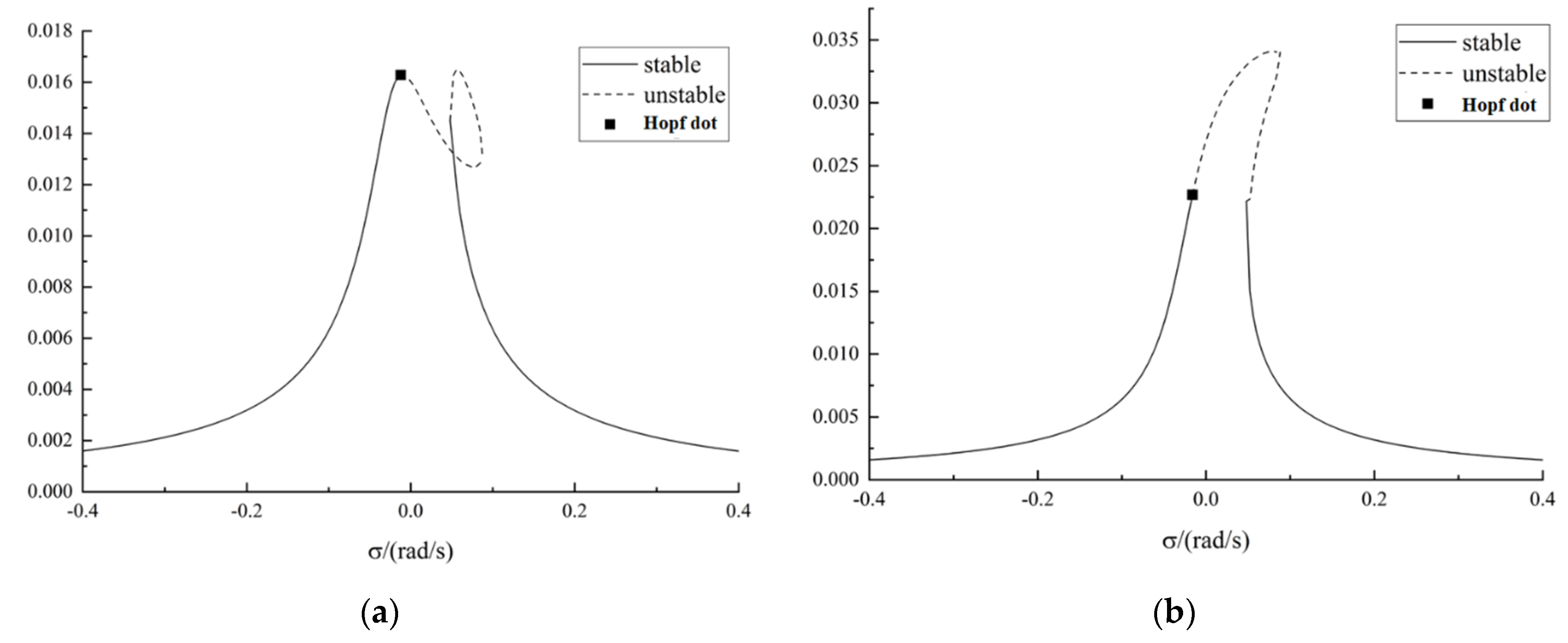
The nonlinear stiffness has a great influence on the nonlinear motion of the pipe. When the nonlinear stiffness increases to a certain extent, saddle-node bifurcation and Hopf bifurcation appear, and the motion form of the pipe is more complex, while the vibration amplitude of the pipe is greatly suppressed. Therefore, the vortex-induced resonance of the pipe can be effectively suppressed by reasonably selecting the nonlinear stiffness of an NES.

(3)

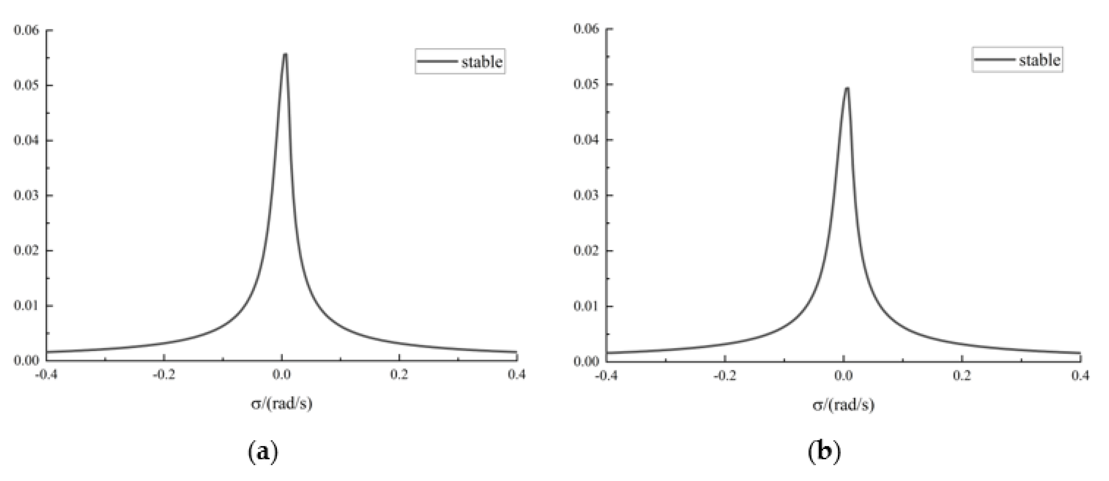
For a system with nonlinear motion, an NES damping mainly affects the range of the unstable region of the pipe. The larger the damping, the smaller the unstable region of the amplitude-frequency response curve. For a system without nonlinear motion, increasing an NES damping will decrease the response amplitude of the pipe near the resonance region. A reasonable combination of nonlinear stiffness and damping should be considered.

The deep-water jacket pipe had a rigid body and only one degree of freedom in this study, and its elasticity should be further studied. In addition, this paper only considers one NES damper, and there will be multiple NESs in practice, which requires further study.

References

1. Jiakun, L. Study on vortex-induced vibration of jacket during construction. Harbin Inst. Technol. 2016. [Google Scholar]
2. Xiaoxu, C.; Rui, W.; Shugeng, Y.; Yang, P.; Yi, L. Calculation method of stroke-induced vibration of jacket during towing. J. Oil Field Equip. 2012, 41, 33–37. [Google Scholar]
3. Chunyan, J. Research on dynamic response analysis and vibration control technology of offshore platform. Ocean. Univ. China 2003. [Google Scholar] [CrossRef]
4. Hermann, F. Device for Damping Vibrations of Bodies. US Patent 0,989,958, 30 October 1909. [Google Scholar]
5. Vakakis, A.F. Inducing Passive Nonlinear Energy Sinks in Vibrating Systems. J. Vib. Acoust. 2001, 123, 324–332. [Google Scholar] [CrossRef]
6. Georgiades, F.; Vakakis, A.F. Dynamics of a linear beam with an attached local nonlinear energy sink. Commun. Nonlinear Sci. 2007, 12, 643–651. [Google Scholar] [CrossRef] [Green Version]
7. Ahmadabadi, Z.N.; Khadem, S.E. Nonlinear vibration control of a cantilever beam by a nonlinear energy sink. Mech. Mach. Theory 2012, 50, 134–149. [Google Scholar] [CrossRef]
8. Zhou, K.; Xiong, F.R.; Jiang, N.B.; Dai, H.L.; Yan, H.; Wang, L. Nonlinear vibration control of a cantilevered fluid-conveying pipe using the idea of nonlinear energy sink. Nonlinear Dyn. 2019, 95, 1435–1456. [Google Scholar] [CrossRef]
9. Zhang, Y.W.; Hou, S.; Zhang, Z.; Zang, J.; Chen, L.Q. Nonlinear vibration absorption of laminated composite beams in complex environment. Nonlinear Dyn. 2020, 99, 2605–2622. [Google Scholar] [CrossRef]
10. Dai, H.L.; Abdelkefi, A.; Wang, L. Vortex-induced vibrations mitigation through a nonlinear energy sink. Commun. Nonlinear Sci. 2017, 42, 22–36. [Google Scholar] [CrossRef]
11. Chen, D.; Abbas, L.K.; Wang, G.; Rui, X.; Pier, M. Numerical study of flow-induced vibrations of cylinders under the action of nonlinear energy sinks (NESs). Nonlinear Dyn. 1992, 94, 925–957. [Google Scholar] [CrossRef]
12. Blanchard, A.B.; Gendelman, O.V.; Bergman, L.A.; Lawrence, A.; Bergman, A.; Alexander, F.; Vakakis, C. Capture into slow invariant manifold in the fluid-structure dynamics of a sprung cylinder with a nonlinear rotator. J. Fluid. Struct. 2016, 63, 155–173. [Google Scholar] [CrossRef] [Green Version]
13. Liqin, L.; Yiqun, C.; Wenjun, S.; Hao, L.; Zhiqiang, W. Study on Wind-induced Vortex- induced Vibration and Vibration Reduction of Tubular Platform under Construction. Ocean Eng. 2021, 39, 1–8. [Google Scholar] [CrossRef]
14. Zheng, L.; Zixin, W.; Xilin, W. Summary of Research on Nonlinear Energy Trapping Technology. J. Vib. Shock 2020, 39, 1–16+26. [Google Scholar] [CrossRef]
15. Wang, L.; Liu, J.; Yang, C.; Wu, D. A novel interval dynamic reliability computation approach for the risk evaluation of vibration active control systems based on PID controllers. Appl. Math. Model. 2021, 92, 422–446. [Google Scholar] [CrossRef]
16. Yiqun, C. Study on Characteristics and Mechanism of Wind-Vortex-Induced Vibration of Jacket Platform; School of Civil Engineering of Tianjin University: Tianjin, China, 2021. [Google Scholar]
17. Jiawei, Z.; Yougang, T.; Yan, L.; Xiaoqi, Q.; Ruoyu, Z. Effect of vortex-induced resonance on motion response of Spar floating fan in wind and wave flow. Ocean Eng. 2018, 36, 39–49. [Google Scholar] [CrossRef]
18. Starosvetsky, Y.; Gendelman, O.V. Attractors of harmonically forced linear oscillator with attached nonlinear energy sink. II: Optimization of a nonlinear vibration absorber. Nonlinear Dyn. 2008, 51, 47. [Google Scholar] [CrossRef]
19. Gendelman, O.V.; Starosvetsky, Y.; Feldman, M. Attractors of harmonically forced linear oscillator with attached nonlinear energy sink I: Description of response regimes. Nonlinear Dyn. 2008, 51, 31–46. [Google Scholar] [CrossRef]
20. Jian, Z. Complex Dynamics Study and Vibration Suppression Evaluation Method of Nonlinear Energy Well; Shanghai University: Shanghai, China, 2021. [Google Scholar]
21. Luongo, A.; Zulli, D. Dynamic analysis of externally excited NES-controlled systems via a mixed Multiple Scale/Harmonic Balance algorithm. Nonlinear Dyn. 2012, 70, 2049–2061. [Google Scholar] [CrossRef] [Green Version]
22. Liu, Y.; Wang, L.; Gu, K.; Li, M. Artificial Neural Network (ANN)-Bayesian Probability Framework (BPF) based method of dynamic force reconstruction under multi-source uncertainties. Knowl.-Based Syst. 2022, 237, 107796. [Google Scholar] [CrossRef]
23. Wang, L.; Liu, Y.; Liu, D.; Wu, Z. A novel dynamic reliability-based topology optimization (DRBTO) framework for continuum structures via interval-process collocation and the first-passage theories. Comput. Methods Appl. Mech. Eng. 2021, 386, 114107. [Google Scholar] [CrossRef]
24. Wang, L.; Liu, Y.; Li, M. Time-dependent reliability-based optimization for structural-topological configuration design under convex-bounded uncertain modeling. Reliab. Eng. Syst. Saf. 2022, 221, 108361. [Google Scholar] [CrossRef]
25. Jinyan, Z.; Jian, X. Vibration reduction mechanism of nonlinear dynamic absorber with time delay. Theor. Appl. Mech. 2008, 1, 98–106. [Google Scholar]
26. Rui, W. Research on Prevention and Control Measures of Wind-Induced Vibration of Jacket during Towing Process; Tianjin University: Tianjin, China, 2012. [Google Scholar] [CrossRef]
Figure 1. Vortex-induced vibration model of a pipe.
Applsci 12 07272 g001
Figure 2. A pipe with unilateral constraint of a jacket platform.
Applsci 12 07272 g002
Figure 3. Response time history diagram when σ = 0, κ = 97.97, ξ2 = 0.0085, ρ2 = 0.02; (a) Analytical solution of x1; (b) approximate analytical solution of Z; (c) numerical solution of x1; and (d) numerical solution of Z.
Applsci 12 07272 g003aApplsci 12 07272 g003b
Figure 4. Response displacement spectrum. (a) Pipe displacement and (b) relative displacement of pipe-NES.
Applsci 12 07272 g004
Figure 5. Amplitude frequency response curve when κ = 97.97, ξ2 = 0.0085, ρ2 = 0.02, (a) pipe displacement amplitude and (b) relative displacement amplitude.
Applsci 12 07272 g005
Figure 6. Amplitude frequency response curve when κ = 24.425, ξ2 = 0.0085, ρ2 = 0.02, (a) pipe displacement amplitude and (b) relative displacement amplitude.
Applsci 12 07272 g006
Figure 7. Amplitude frequency response curve when κ = 367.38, ξ2 = 0.0085, ρ2 = 0.02, (a) pipe displacement amplitude and (b) relative displacement amplitude.
Applsci 12 07272 g007
Figure 8. Response under different initial conditions (κ = 367.38, ξ2 = 0.0085, ρ2 = 0.02, σ = −0.144), (a) x1 at initial condition (0, 0, 0, 0), (b) x1 at initial condition (3, 3, 3, 3), (c) Z at initial condition (0, 0, 0, 0), (d) Z at initial condition (3, 3, 3, 3).
Applsci 12 07272 g008
Figure 9. Comparison of amplitude–frequency response curves of the pipe.
Applsci 12 07272 g009
Figure 10. Amplitude frequency response curve when κ = 367.38, ξ2 = 0.0044, ρ2 = 0.02, (a) pipe displacement amplitude and (b) relative displacement amplitude.
Applsci 12 07272 g010
Figure 11. Amplitude frequency response curve when κ = 367.38, ξ2 = 0.0117, ρ2 = 0.02, (a) pipe displacement amplitude and (b) relative displacement amplitude.
Applsci 12 07272 g011
Figure 12. Comparison of pipe response of different parameters, (a) response (κ = 367.38, ρ2 = 0.02), (b) response (κ = 24.425, ρ2 = 0.02).
Applsci 12 07272 g012