The Cube Surface Light Field for Interactive Free-Viewpoint Rendering

Abstract

Free-viewpoint rendering has always been one of the key motivations of image-based rendering and has broad application prospects in the field of virtual reality and augmented reality (VR/AR). The existing methods mainly adopt the traditional image-based rendering or learning-based frameworks, which have limited viewpoint freedom and poor time performance. In this paper, the cube surface light field is utilized to encode the scenes implicitly, and an interactive free-viewpoint rendering method is proposed to solve the above two problems simultaneously. The core of this method is a pure light ray-based representation using the cube surface light field. Using a fast single-layer ray casting algorithm to compute the light ray’s parameters, the rendering is achieved by a GPU-based three-dimensional (3D) compressed texture mapping that converts the corresponding light rays to the desired image. Experimental results show that the proposed method can real-time render the novel views at arbitrary viewpoints outside the cube surface, and the rendering results preserve high image quality. This research provides a valid experimental basis for the potential application value of content generation in VR/AR.

1. Introduction

Image-based rendering is a technique of generating a rendering result of an unknown viewpoint by interpolating through the collected image dataset [1]. One of its research motivations is the free-viewpoint rendering, i.e., to synthesize images at arbitrary viewpoints from discrete as well as sparse pre-captured images using appropriate transformations [2,3]. This kind of method does not require building three-dimensional (3D) mesh models of the scene in advance, and has broad application prospects in content generation, especially in the field of virtual reality and augmented reality (VR/AR). However, existing free-viewpoint rendering mainly adopts either the traditional image-based methods or the learning-based frameworks, and there are still many problems to be further studied.

One of the problems is the limited viewpoint freedom. The core of traditional image-based methods is the multidimensional representation of the light field [4] which describes the intensities of light rays passing through any viewpoints and any directions in free space. Restricting the light field in different dimensions can derive different kinds of light field representations, thus limiting the freedom of viewpoint to varying extents. For example, the two-parallel-plane parameterized (2PP) four-dimensional (4D) light field L(u, v, s, t) limits the viewpoints on a specific plane (camera plane) [5,6]. The 3D light field, such as the concentric mosaic, limits the viewpoints to a specific viewing circle (camera circle) [7,8,9,10]. The simplest 2D light field representation, i.e., the panorama limits the viewpoints to a single projection center [11,12,13,14]. The constraint on viewpoint freedom is helpful to simplify the dimensions of the light field model as well as reduce its data complexity. However, the free-viewpoint rendering pursues that the desired images can be rendered at arbitrary positions and orientations in the observation space. The above methods limit the degree of freedom (DoF) of the viewpoints so that the systems based on these methods only provide restricted viewpoints which does not satisfy the natural interaction between human and the real-world scenes.

Another problem is the poor time performance of novel view rendering. With the rapid progress of deep learning, some researchers use the learning-based frameworks to generate arbitrary views [15,16,17,18], trying to alleviate the restriction of the DoF of the viewpoints. However, this kind of method requires a complex training process, expensive network computation and takes a lot of time as well as memory for generating a high-resolution novel view, which cannot guarantee the real-time rendering performance. Both of these two issues have to be solved in the applications of free-viewpoint rendering in VR/AR. Only by providing a full viewpoint coverage in the observation space as well as the real-time rendering performance, can we meet the requirement of content generation in VR/AR [19].

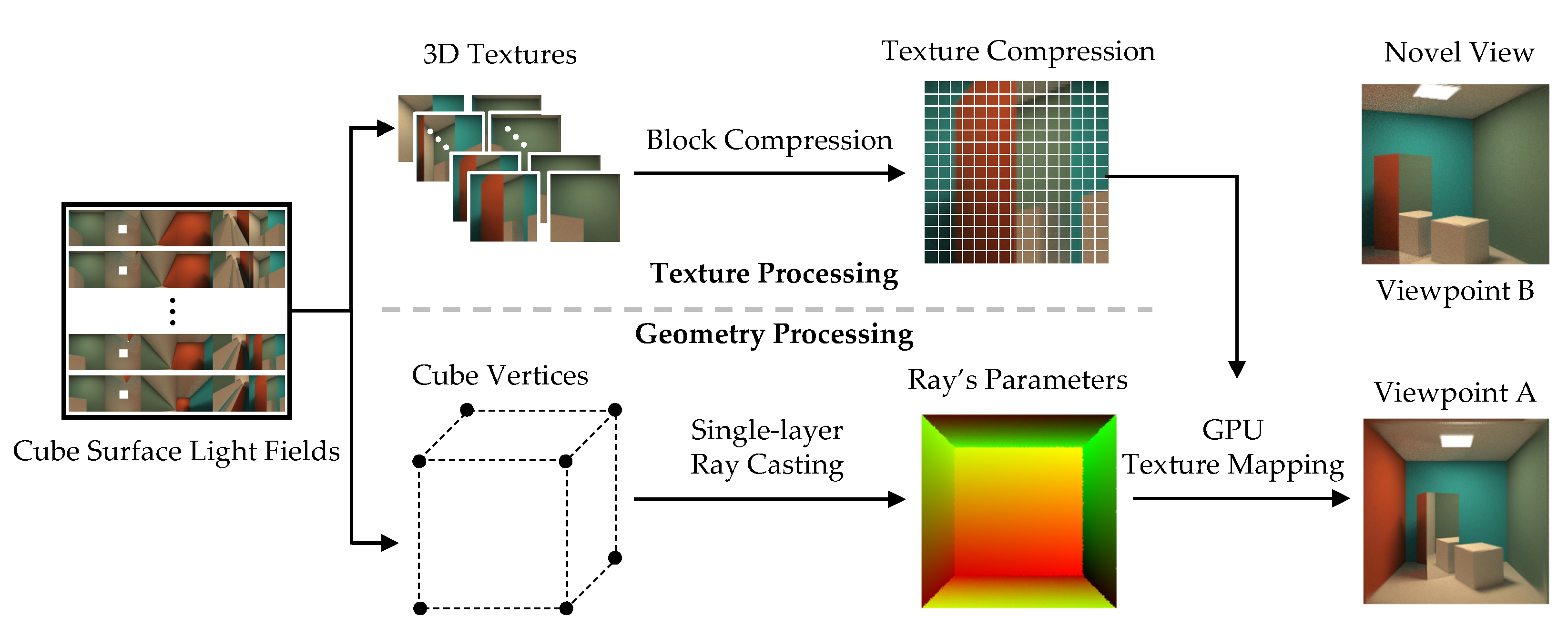
In this paper, we present an interactive free-viewpoint rendering method using the cube surface light field which is a pure light ray-based scene representation. The complexity of this representation is independent of the scene’s geometric structures, indicating its ability to represent anisotropic light fields in arbitrary scenes by a unified model. The basic pipeline of our method is shown as Figure 1. Firstly, based on the pure light ray-based scene representation, the input of our method is the cube surface light fields consisting of a certain number of pre-collected images. Then, our method is divided into two independent steps: texture processing and geometry processing. In texture processing, we use the 3D texture compression algorithm to process the cube surface light field images, making its data amount acceptable to personal computers. In geometric processing, we adopt the programmable rendering pipeline from cube vertices to frame buffer and use a fast single-layer ray casting algorithm to render a unit cube mesh as well as computing the parameters of the desired light rays that are finally used for GPU texture mapping, converting a group of light rays to a novel view. Given different target viewpoints, our method can render the corresponding novel views such as viewpoint A and B in Figure 1.

Compared with the mesh-based rendering, our rendering method is not affected by the specific geometric structures of the scenes and can be extended to arbitrary scenes using a unified model, i.e., the cube surface light field representation. Moreover, our method does not need to solve the integral of the rendering equation for each frame, which greatly reduces the computational consumption during the rendering. Compared with the traditional image-based rendering, the proposed method greatly improves the DoF of the viewpoints, which can render the novel views at arbitrary positions and viewing directions outside the cube surface. Compared with the learning-based methods, the proposed method can achieve interactive rendering (IR), and the average frame rate for rendering a novel view with a resolution of 2048 × 2048 on a personal computer can reach more than 75 FPS. In summary, the main contributions of this paper are as follows:

• a pure light ray-based representation that supports implicitly encoding the scenes to a unified model,
• a free-viewpoint rendering method based on compressed texture mapping and ray casting, which supports rendering the novel views without any explicit geometry structures of the scenes, significantly improving the DoF as well as the time performance of novel view light field rendering with high resolution.

2. Related Work

In the past few years, the free-viewpoint rendering technology has gained a growing attention from both academia and industry, and has also made promising progress. The existing methods can be mainly divided into three categories: mesh-based methods, traditional image-based methods, and learning-based methods. In this section, we give a brief review on recent works related to our work.

2.1. The Mesh-Based Methods

Mesh-based rendering is one of the most widely-used methods. It uses a 3D mesh model to represent the geometric structures of the scene and renders the desired views with various materials of the scenes using the classical illumination methods under the given viewpoint parameters [20]. To further improve the illumination reality of the scenes, some researchers have proposed various global illumination rendering algorithms, such as ray tracing, path tracing, and photon mapping [21]. However, these global illumination algorithms require a lot of computational resources, and the rendering for a single view usually takes more time than the rendering using classical illumination methods. For example, it takes more than two or three hours to render a single indoor scene with a resolution of 2048 × 1024 using a POV-Ray ray tracing renderer [22]. Although the advanced game engine [23] can achieve real-time ray tracing, it also requires the scene-by-scene optimization as well as the support of advanced hardware, e.g., Nvidia RTX.

2.2. Traditional Image-Based Methods

The image-based methods take the convenience of capturing images to solve the rendering of the geometry-complex scenes from the perspective of image processing, relieving the requirement of geometric pre-modeling of the scenes. This kind of method mainly focuses on the light field representation [4]. Due to the high-dimensional characteristics of the light field, obtaining a complete light field always consumes many resources including both time and space. The recently proposed methods try to simplify the light field from different dimensions to generate the simplified light field representations and to solve the rendering for the specific scenes [24,25,26]. For example, the 2PP light field simplifies the seven-dimensional (7D) plenoptic function L(x, y, z, $\theta$, $\varphi$, $\lambda$, t) (the wavelength $\lambda$ of an arbitrary light ray in the direction of ($\theta$, $\varphi$) from the position of (x, y, z) at time t) to a 4D light field function by restricting the viewpoints on a plane. The concentric mosaic further restricts the viewpoint on a regular circle [8,25], deriving a 3D representation of the light field. In computer graphics, the simplest representation of the light field is the panorama, which describes all the light rays from all directions in the observation space to a fixed viewing position. It has been widely used for content generation in VR [11,26]. This kind of method limits the DoF of viewpoints to varying extents and thus does not provide the real free-viewpoint rendering.

2.3. Learning-Based Methods

With the development of machine learning and deep learning, the research on the neural representation of the scenes has gradually increased. As a representative work, NeRF [15] pushes the neural scene representation to a new high level [27,28]. Related works based on the NeRF, including NeRF in the wild [29], NeRF body [30], and Point-NeRF [31], Human-NeRF [32], extend the NeRF to various applications. A comprehensive review of neural rendering has been reported in [33]. This kind of method mainly establishes the neural representation of the scenes from the pre-captured images, and then renders the desired views through various network structures. Some methods support rendering novel views from relatively sparse pre-captured images and even achieve the free-viewpoint rendering [34]. However, these methods require an expensive per-scene optimization process which takes a lot of time and memory for rendering a single view. For example, NeRF takes hours or days to optimize a specific scene [15]. The real-time performance using the neural scene representations remains to be further studied.

3. Cube Surface Light Field Representation

The core idea of the cube surface light field representation is to parameterize the light rays on the two intersections with the cube surface and use the color value at the first intersection of the light ray and the object’s surface to be the color of this light ray, constructing a pure ray-based 4D light field representation of the scenes, as shown in Figure 2.

The light rays in free space can be divided into two categories. The first category of light ray does not intersect with the objects in the scene, and almost does not influence the objects’ appearance. The second category of light ray intersects with the scene’s objects and has a significant impact on the objects’ appearance, resulting in light and dark effects on the objects’ surfaces. The origination of such light rays either can be from one or more light sources or can be the reflected light rays on the surface of an adjacent object. In particular, the images captured by a camera have already encoded the final impact of the light rays from these two originations on the appearance of the scene. Therefore, only the second category of light ray is concerned in the study of free-viewpoint rendering, and we do not distinguish whether the light ray is from the light source or the reflection from the adjacent objects’ surface.

The cube surface light field uses a unified cube geometry to parameterize the set of the second category of light ray in free space and uses the pairs of intersected points on the cube surface to be the parameters of light rays. We define that the center of the cube geometry is located at the origination of the 3D Cartesian coordinate system (CCS), and the edge length is the same as the size of the scene’s bounding box. According to the twelve edges of the cube geometry, its surface can be divided into six sub-planes, corresponding to +X, +Y, +Z, −X, −Y, −Z planes, respectively. Therefore, the cube surface can be defined by a 2D function composed of six sub-planes, as shown in Equation (1), in which (x, y) refers to the 2D coordinates of the interior points on each sub-plane.

$$\begin{array}{c}\mathrm{C}:{\displaystyle \sum _{i=1}^6}{\Pi }_i(x,y)\subset {\mathbb{R}}^2\end{array}$$

(1)

On the cube surface, the origination of each light ray is defined by the 2D coordinates at the first intersections with the light rays and the cube surface, and the directions of the light rays are defined by the 2D coordinate at the second intersections with the light rays and the cube surface. The color values of each light ray are defined as the color at the first intersections with the light rays and the scenes, which are described by the RGB color representation. Consequently, the cube surface light field can be defined as a set of RGB color values of the light rays parameterized by the intersection pairs with a specific cube surface, as shown in Equation (2), in which m and n refer to the serial number of the sub-plane where the originations and directions of the light rays are parameterized. Similarly, (u, v) and (s, t) refer to the 2D coordinates of arbitrary interior points on the m-th sub-plane and on the n-th sub-plane, respectively.

$$\mathrm{L}:\sum _{m=1}^6\left({\Pi }_m(u,v)\times \sum _{n=1}^6{\Pi }_n(s,t)\right)\to \mathrm{RGB}$$

(2)

Obviously, for all the light rays that intersect with the scene, the two intersections with the cube surface cannot be on the same sub-plane of the cube surface. Therefore, m and n must not get the same value at the same time in the cube surface light field. According to Equation (2), each light ray has been defined as a six-tuple (m, u, v, n, s, and t) so far. Since m and n are both enumeration values, their definition domains are integers between [1, 6]. To facilitate the parametric representation of the light field, the cube surface, as shown in Figure 3a can be expanded along any of its twelve edges, producing different cube map layouts, such as vertical and horizontal cross layouts, as shown in Figure 3b. We use the horizontal layout as shown in Figure 3c to present each sub-view of the cube surface light field.

Intuitively, the texture coordinates can be used to further simplify Equation (2), resulting in the final representation of the cube surface light field denoted by Equation (3). Seeing from the dimension of u and v, each coordinate (u, v) represents a set of light rays from a fixed position, which can be described as a light field sub-view like in the traditional 2PP light field representation. Meanwhile, seeing from the dimension of s and t, each coordinate (s, t) represents a set of light rays from a fixed direction, which can be described as a sub-aperture image like in the 2PP light field representation.

$$\mathrm{L}:\mathrm{I}(u,v)\times \mathrm{I}(s,t)\to \mathrm{RGB}$$

(3)

One advantage of the cube surface parameterization is that it is easy to sample the light field. The two adjacent edges of each sub-plane are divided into several segments uniformly or non-uniformly. By connecting the endpoints of the two opposite segments, the sub-plane can be subdivided into several small square or rectangular blocks. The barycentric coordinates of each square or rectangular can be selected as the sampling points of the cube surface light field. This representation also helps to compress the light field images at each sampling point. The images generated by the sampling points on the same sub-plane have only translational transformation in both horizontal and vertical directions. If the equidistant sampling strategy is adopted in the sampling stage, the relationship between the image pixels of these viewpoints is easy to be quantitatively described by parallax, which facilitates the prediction and compression of adjacent views. It is also conducive to subsequent rendering, i.e., the light field rendering of an arbitrary scene only requires drawing a simple unit cube geometric. By intersecting the desired light rays with the cube surface, the light ray’s parameters can be computed and used to query the color value of the novel viewpoint pixels. The computational consumption for testing intersection with the light rays and cube surface is relatively low, which makes the cube surface light field rendering possible to achieve real-time performance.

4. Ray Casting Based Interactive Novel View Rendering

The rendering of the cube surface light field can be achieved by a general cube geometric proxy which can be rendered by the traditional rasterization or ray casting algorithm. To improve the computational efficiency of the ray parameters, we use a ray casting algorithm for fast ray computation of the cube surface light field and use GPU 3D texture mapping to convert light rays into pixel colors in the frame buffer. The rendering framework, as shown in Figure 1, mainly includes texture processing and geometry processing.

4.1. Texture Processing

The texture processing is to pre-process the cube surface light field images, generate 3D textures from multi-view images, and compress the 3D textures to reduce the texture memory required during the rendering.

4.1.1. 3D Texture Generation

The representation of the cube surface light field is a set of cube maps and each cube map is arranged linearly from +X to −Z, as shown in Figure 3c. According to the position of each viewpoint in the sampling points, an image matrix with m rows and n columns can be generated directly for each cube face, as shown in Equation (4), where ${\mathrm{I}}_{ij}$ represents the cube map in the i row and the j column.

$${\mathrm{M}}_{m\times n}=\left[\begin{array}{ccc}{\mathrm{I}}_{00}& ...& {\mathrm{I}}_{0n}\\ ...& {\mathrm{I}}_{ij}& ...\\ {\mathrm{I}}_{m0}& ...& {\mathrm{I}}_{mn}\end{array}\right]$$

(4)

To generate a 3D texture, it requires to convert the 2D matrix of images, i.e., Equation (4) into a linear space. Therefore, we adopt the transverse scanning strategy (zigzag) to transform the image matrix, and the depth of 3D texture z is simply computed by $z_{(i,j)}=m\ast j+i,z\in [0,i\ast j)$. Each sub-plane can be represented as a 3D texture ${\mathrm{T}}_i$(d, x, y) denoted as Equation (5), where x and y represent the image coordinates of the cube surface light field, respectively.

$$\begin{array}{c}\hfill {\mathrm{T}}_i(z,x,y)=\left[{\mathrm{I}}_{z_{(0,0)}}(x,y),\dots ,{\mathrm{I}}_{z_{(0,n)}}(x,y),\dots ,\right.\\ \hfill {\mathrm{I}}_{z_{(0,n)}}(i,j),\dots ,{\mathrm{I}}_{z_{(m,0)}}(x,y),\\ \hfill \left.\dots ,{\mathrm{I}}_{z_{(m,n)}}(x,y)\right]\end{array}$$

(5)

4.1.2. Block Compression

The data amount of 3D textures generated in the previous stage is usually very large. For a light field with a resolution of $m\times n\times w\times h$, the memory of a single 2D texture is $w\times h\times 4$ bytes and the memory of all textures is $m\times n\times w\times h\times 4$ bytes. Here, $m\times n$ refers to the rows and columns of the image matrix, i.e., the angular resolution of this light field, and $w\times h$ refers to the pixel width and height of each image, i.e., the spatial resolution of this light field. For example, when an RGBA light field with a resolution of $100\times 100\times 512\times 512$ is assumed to occupy 8-bit for each channel, it means that the angular resolution of this light field is $100\times 100$ and the spatial resolution is $512\times 512$. Moreover, if we use the In-Core texture mapping strategy, it requires 9.8 GB of memory in the rendering.

Obviously, rendering directly using the uncompressed texture mapping strategy is not realistic for personal computers. To reduce the texture memory required for the cube surface light field rendering, these 3D textures are compressed in the block compression stage. First, each texture in the 3D texture is divided into several sub-blocks, each containing 4 × 4 pixels. Since the light field data is usually used to describe the color appearance of the scene, in each $4\times 4$ pixel block, the colors in these 16 pixels have little change, as shown in Figure 4, indicating that a color disk with only a few colors can be used to represent the whole $4\times 4$ pixel block, and the color of each pixel in the sub-block can be computed according to the color disk and a set of coefficients. Since each sub-block is only represented by a color disk with a few colors, the storage required for this 3D texture can be reduced. Assuming that the colors in the disk are evenly distributed in the linear color space defined by the gray scale of the RGB value using the transformation of $Y=0.3\ast R+0.59\ast G+0.11\ast B$, the colors and coefficients of two endpoints ($Y_{max}$ and $Y_{min}$) can be used to further compress the color disk. The compressed texture first store two endpoints of the linear color space and all other colors can be obtained by interpolating these two endpoints with different coefficients.

Because the pixels of the light field images are represented by four-channel RGBA, in order to obtain a larger compression rate, 8 bytes are used to store each $4\times 4$ pixel block in the block compression stage, so that each pixel can be represented by an average of 0.5 bytes. The file for each block includes two endpoints of color, which are the brightest ($c_0=Y_{max}$) and darkest ($c_3=Y_{min}$) color values in these 16 pixels. Both colors are stored in R5G6B5 format, i.e., 5 bits, 6 bits, 5 bits per channel, and 2 bytes per color. Since there is no transparency in the cube surface light fields, the A channel here can be ignored. In addition, two additional colors are used to further improve the compression rate, which are computed by Equation (6) with $\alpha =2/3$, $\beta =1/3$ for $c_1$ and $\alpha =1/3$, $\beta =2/3$ for $c_2$.

$$Z=\alpha \ast X+\beta \ast Y$$

(6)

Therefore, each $4\times 4$ pixel block are represented by four colors $c_0$, $c_1$, $c_2$, $c_3$. At the same time, each block contains 16 pixels, and 16 coefficients are required to represent all the pixel colors. Each index requires two bits of memory cost, and an additional four bytes are required to store all the 16 indexes. The color of each pixel in the pixel block is encoded by the nearest color in four colors, and is represented by a query table: $c_0:00$, $c_1:01$, $c_2:10$, $c_3:11$. With the block compression, the data amount of each pixel block can be reduced to 1/8. In our experiments, we use DirectDraw Tex to compress the light field images into a separate DirectDraw Surface (DDS) container and then pass the DDS file to the fragment shader as a 3D texture for the subsequent GPU texture query of light rays.

4.2. Geometry Processing

The purpose of geometry processing is to compute the parameters of the desired light rays and to query each ray’s color from the cube surface light field textures. Since we use a unified cube geometry to parameterize the light rays by two intersections. This makes it possible to compute the desired light rays parameters only by computing the two intersection points between the rays emitted from the viewpoint and the cube surface. Since the cube surface light field uses the cube map to store the light rays, the color value of the corresponding light rays can be directly fetched by texture mapping, and the computational complexity of the light ray query is O(1).

Figure 5 shows the relationship between an arbitrary pixel in the image plane of a novel viewpoint and the cube surface light field. Given the viewpoint parameters (camera parameters), all the light rays from this viewpoint to each pixel in the image plane can be defined, and the intersection points between each light ray and the cube surface can also be computed. Both generating light rays from the viewpoint to the image plane and testing intersections can be achieved by a single-layer ray casting. Different from traditional ray casting, single-layer ray casting only needs to query the pixel colors from the outermost image, instead of superimposing the pixel colors of all the intersected images.

Due to the simplicity and regularity of the cube surface, computing the intersections is so simple that the cube surface light field rendering can achieve real-time performance on personal computers. After computing the light rays parameters, we need to query the color of these light rays. If the desired light ray is just located at a sampled point, the sampled color can be used for the color of this light ray. If the desired light ray is located in the under-sampled regions, different interpolation rendering can be used in texture mapping to blend the adjacent sampled light rays. In the cube surface light field rendering, the nearest neighbor interpolation (NNI), linear interpolation (LI), and bilinear interpolation (BLI) algorithms can be used to deal with those under-sampled light rays. In this paper, bicubic interpolation (BCI) and cubic B-spline interpolation (CBSI) algorithms are expanded to further reduce the aliasing artifacts. Algorithm 1 describes the pipeline of rendering novel views from arbitrary viewpoints.

Algorithm 1 Interactive Novel View Rendering

Input:  The set of block compressed light fields, $\mathit{L}$; The cube geometry, $\mathit{C}:\{{\mathit{v}}_{\mathit{max}},{\mathit{v}}_{\mathit{min}}\}$; The current camera matrix, ${\mathit{M}}_{4\times 4}:\{{\mathit{v}}_{\mathit{pos}},{\mathit{v}}_{\mathit{directions}}\}$; Output:  The frame buffer for novel view, $\mathit{I}$; 1: Clear all the pixel colors in $\mathit{I}$ to $0x000000$; 2: for all pixels $P(x,y)$∈ the image plane do 3:   Generate a camera ray ${\mathit{r}}_{\mathit{i}}$ from $v_{pos}$ to $p_i(x,y)$, ${\mathit{r}}_{\mathit{i}}=\mathit{v}+t\ast \mathit{d}$; 4:   ${\mathit{t}}_{\mathit{min}}=\min (({\mathit{v}}_{\mathit{min}}-\mathit{v})/\mathit{d},({\mathit{v}}_{\mathit{max}}-\mathit{v})/\mathit{d})$; 5:   ${\mathit{t}}_{\mathit{max}}=\max (({\mathit{v}}_{\mathit{min}}-\mathit{v})/\mathit{d},({\mathit{v}}_{\mathit{max}}-\mathit{v})/\mathit{d})$; 6:   $t_0=\max (\max ({\mathit{t}}_{\mathit{min}}.x,{\mathit{t}}_{\mathit{min}}.y),{\mathit{t}}_{\mathit{min}}.z)$; 7:   $t_1=\min (\min ({\mathit{t}}_{\mathit{max}}.x,{\mathit{t}}_{\mathit{max}}.y),{\mathit{t}}_{\mathit{max}}.z)$; 8:   if $t_0<t_1$ and $t_0>0.0$ then 9:      ${\mathit{v}}_{\mathbf{0}}=\mathit{v}+t_0*\mathit{d}$; 10:    ${\mathit{v}}_{\mathbf{1}}=\mathit{v}+t_1*\mathit{d}$; 11:    Get the texture coordinates of ${\mathit{v}}_{\mathbf{0}}$ and ${\mathit{v}}_{\mathbf{1}}$, ${\mathit{v}}_{\mathbf{0}}⟶(u_i,v_i)$, ${\mathit{v}}_{\mathbf{1}}⟶(s_i,t_i)$; 12:    Select N rays $(u_j,v_j,s_j,t_j)$ adjacent to $(u_i,v_i,s_i,t_i)$; 13:    ${\mathit{I}}_{p_i(x,y)}={\displaystyle \sum _{j=1}^N}\mathit{L}(u_j,v_j,s_j,t_j)\ast {\omega }_j$; 14:  end if 15: end for

4.2.1. Bicubic Interpolation Rendering

Without losing generality, assuming a ray passing through a direction ($s^{*}$, $t^{*}$) is under-sampled, BCI rendering requires searching for the adjacent sampled light rays in the u and v dimensions. For each under-sampled light ray, the 4 × 4 adjacent sampled light rays are selected and blended according to the specific weights. The blending equation can be described as Equation (7).

$$\mathrm{L}(u,v,s*,t*)=\sum _{i=0}^3\sum _{j=0}^3\mathrm{L}(u_i,v_j,s*,t*)\ast \omega (u_i,v_j)$$

(7)

where the weight $\omega (u_i,v_j)$ is computed by Equations (8) and (9).

$$\omega (u_i,v_j)=\omega \left(d_{u_i}\right)\ast \omega \left(d_{v_j}\right)$$

(8)

$$\omega \left(d\right)=\left\{\begin{array}{c}(a+2)\ast {\left|d\right|}^3\hfill \\ -(a+3)\ast {\left|d\right|}^2+1,\hfill & \mathrm{if}\left|d\right|\le 1\hfill \\ a\ast {\left|d\right|}^3\hfill \\ -5\ast a\ast {\left|d\right|}^2\hfill \\ +8\ast a\ast \left|d\right|-4\ast a,\hfill & \mathrm{if}1<\left|d\right|\le 2\hfill \\ 0,\hfill & \mathrm{otherwise}\hfill \end{array}\right.$$

(9)

in which the range of a is (−1, 0), and generally it is taken as a fixed value, i.e., $-0.5$. The distances $d_x$ and $d_y$ are computed by Equation (10) and Equation (11), respectively.

$$d_{u_i}=u_i-u$$

(10)

$$d_{v_j}=v_j-v$$

(11)

Similarly, assuming that a light ray passing through a position ($u^{*}$, $v^{*}$) is under-sampled, the color of this light ray can be computed by blending the corresponding light rays in the s and t dimensions using Equation (7).

4.2.2. Cubic B-Spline Interpolation Rendering

For those under-sampled light rays, the CBSI rendering selects the $4\times 4$ adjacent sampled light rays and blends them according to the different weights. This blending equation is the same as Equation (7), and the difference is the computation of $\omega \left(d\right)$ which is defined by Equation (12).

$$\omega \left(d\right)=\left\{\begin{array}{cc}\frac{2}{3}-(1-\frac{\left|d\right|}{2})\ast {\left|d\right|}^2,\hfill & \mathrm{if}\left|d\right|\le 1\hfill \\ \frac{1}{6}\ast {(2-\left|d\right|)}^3,\hfill & \mathrm{if}1<\left|d\right|\le 2\hfill \\ 0,\hfill & \mathrm{otherwise}\hfill \end{array}\right.$$

(12)

It is worth noting that the cube surface light field is represented by a set of cube maps. In the light ray query stage, it is necessary to implement the viewpoint space ray query as well as the image space ray query. The above two interpolation methods can be used when querying light rays by texture mapping, and in general, CBSI can achieve better anti-aliasing effects. Considering that the resolution of the image space is much larger than that of the viewpoint space, in order to reduce the computational consumption, simple interpolation methods such as NNI and LI are used for the light ray query. For the query in the viewpoint space, it is necessary to use an appropriate interpolation algorithm such as CBSI to avoid a large computation deviation of light rays.

5. Results and Discussion

We use OpenGL and GLSL to implement the proposed rendering method on a personal computer with Intel Xeon(R) CPU E5-1650v4 @3.60 GHz CPU, 16 GB RAM, and Nvidia Quadro P4000 GPU. In this section, we first analyze the DoF of renderable viewpoints in ray space. Then, we study the time performance of our method and compare it with the path tracing rendering. The quality of images rendered by various interpolations and path tracing are evaluated finally.

5.1. Ray Space Analysis

The cube surface light field is presented by a set of cube maps arranged by the texture coordinates, i.e., the sampling points. Each sampling point in the viewpoint space represents all the light rays starting from this point to the whole image space. All the sampling points in the viewpoint space amalgamated to form a viewpoint cube map. Therefore, the coverage of the viewpoint cube map has an important impact on the DoF of the subsequent rendering.

Considering that it is easier to understand the light ray’s distribution in ray space, we convert the light rays in 3D space (Cartesian coordinate system, CCS) to ray space (Polar coordinate system, PCS). Without losing generality, the light ray’s projection on the XOY plane is taken as an example to analyze the ray space distributions. Given an arbitrary light ray R in 3D space, its projection on the XOY plane can be marked as Figure 6a. The angle with the +X axis is denoted as $\theta$ and the distance between this projection line to the origin of CCS is denoted as r. Taking $\theta$ and r to be the two coordinate axes of the new coordinate system, this light ray R is converted from CCS to PCS, as shown in Figure 6b. We define the domain of $\theta$ as from $-\pi$ to $\pi$. When a light ray intersects with the positive of the X-axis in CCS, r is positive. On the contrary, r is negative. Each light ray is marked by a black dot and all the light rays constitute the shaded area in PCS.

The traditional 2PP light field has been widely studied, and its light ray’s spatial distributions are shown in Figure 6c,d. It can be seen that the 2PP light field can only represent a subset of light rays, and cannot completely describe the light rays in the whole observation space. Therefore, only a part of viewpoint images can be provided in the rendering stage.

Figure 6f shows the light ray’s distribution of the cube surface light field in ray space. It can be seen that the angular domain $\theta$ is symmetric in ($-\pi$,$\pi$), which covers the whole observation space outside the cube surface. The domain of the light ray’s distance r is symmetric on ($-a$, a) where a is half of the square of the diagonal length, and the light rays are uniformly distributed in the closed area composed of $\theta$ and r.

5.2. Time Performance

To evaluate the time performance of the proposed method, we use a cube surface light field of the Cornell Box with a resolution of $64\times 64\times 256\times 256$ for all of our experiments. The under-sampled light rays are all processed by the CBSI, and the images with the resolutions of $512\times 512$, $1024\times 1024$, $2048\times 2048$, $4096\times 4096$ are rendered for this evaluation. We count the frame rate of generating 100 novel views using our interactive rendering as well as the path tracing rendering with the corresponding resolutions. The comparisons of these two kinds of frame rates are shown in Figure 7. It is worth noting that the frame rate of the path tracing rendering refers to the time consumption when each pixel represents by only one light ray. Although the configuration in the path tracing rendering will lead to aliasing artifacts, this evaluation only considers the time performance of different methods.

It can be seen that different rendering resolutions have little influence on the frame rate. With the improvement of rendering resolution, the frame rate does not decrease or increase significantly. This is because 3D texture mapping is implemented in GPU with parallel acceleration. Under the same rendering resolution, our method can get a higher frame rate than the path tracing rendering, and the highest frame rate reaches more than 250 FPS. In contrast, the average frame rate of the path tracing rendering is about 30 FPS, indicating that our method gets better time performance. This is because our rendering only requires querying light rays from the pre-sampled cube surface light field, and the complexity for the light ray query is O(1) by using compressed 3D texture mapping.

At the same time, we also count the frame rate when using different interpolation methods (NNI, LI, BLI, BCI, and CBSI) to render novel views with a fixed image resolution of $2048\times 2048$ pixels. As can be seen from Figure 8, different interpolation methods have an obvious influence on the rendering frame rate, and more complex interpolation methods will appropriately reduce the frame rate of interactive novel view rendering. This is because the complex interpolation algorithm requires blending more light rays, which increases the computation consumption. When the CBSI is used for processing the under-sampled light rays, the average frame rate of the proposed method is about 75 FPS (the lowest average frame rate), i.e., the worst-case can still meet the real-time requirement for human eyes. This is due to the simplicity of our single-layer ray casting algorithm and the GPU parallel acceleration of the light ray query, making the rendering in real-time.

In this evaluation, the memory usage of our method is about 384 MB for the cube surface light field images, while the memory usage of the path tracing rendering is almost negligible because of the geometric simplicity of the Cornell Box scene. Our method uses the cube surface light field to encode the whole scene’s geometry and appearance. In contrast to traditional mesh-based methods, our method does not depend on the geometric complexity of the scene, i.e., the geometric complexity of the scene can hardly influence the rendering efficiency. However, the traditional mesh-based methods must consider the rendering overhead caused by various scenes’ geometric structures. Moreover, mesh-based large scene rendering is still a problem to be further studied. Compared with the learning-based methods, our method can achieve interactive free-viewpoint rendering. For example, the local light field fusion [6] limits the viewpoints of the light field in a local small range, while the viewpoint of our method is arbitrary in arbitrary positions and directions outside the cube surface. NeRF [15] takes a lot of time to render a single image while our method can reach more than 75 FPS on a personal computer with moderate configurations.

In addition, the proposed method is compared with a related method, i.e., 2PP light field to study its performance. To ensure the fairness of this experiment, we use the same approach, i.e., CBSI to render the 2PP light field. The difference is that the input data is no longer the cube surface light field images of the Cornell Box scene but the 2PP light field images which viewpoints are co-planar and imaging planes are also located on a common plane. We report the average frame rate and memory usage of our method and 2PP method when rendering 100 novel views with a resolution of $2048\times 2048$ pixels, as shown in

Table 1. Comparison of memory usage and frame rate between our method and the 2PP light field.

Item	Method
	2PP Light Field Rendering	Cube Surface Light Field Rendering
Memory Usage (MB)	128	384
Average Frame Rate (FPS)	75	75

. The similar results should be extended to other resolutions and interpolations.

As can be seen from Table 1, the average frame rate of 2PP light field rendering is basically the same as our method, but the memory usage is less than the proposed method. This is because 2PP light field only represent a subset of light rays in the scene, which reduces the total light field data amount but also limits the DOF of rendering viewpoints. On the contrary, by sampling all the light rays on the cube surface, our method can provide free-viewpoint rendering, even though the data amount is greater than the 2PP light field.

5.3. Rendering Quality

To evaluate the quality of images rendered by our method, we use the cube surface light field with a resolution of $64\times 64\times 256\times 256$ and compare the images rendered by several light field interpolation methods with the images rendered by the path tracing. Partial images rendered with a resolution of 2048 × 2048 pixels are shown in Figure 9.

As can be seen from Figure 9, the rendering results by the cube surface light field can reconstruct the global illumination effect of the scene. Especially, a more accurate global illumination effect can be rendered when a more appropriate interpolation method is used. For example, the NNI rendering produces aliasing artifacts, while the CBSI rendering produces smoother images. It also proves from another aspect that our method can be used to accelerate the path tracing rendering. This is because our method records the light rays generated by the path tracing rendering in advance, and only a light ray query is needed in the rendering stage.

To further illustrate the quality of rendered images, we use the non-reference image evaluation indexes, BRISQUE [36] and NIQE [37] to evaluate all images in viewpoint A and report the results in

Table 2. The BRISQUE and NIQE evaluations on the novel views rendered by different methods. The green number indicates the best result among the different interpolation methods, and the red number indicates that path tracing method gets better results.

Viewpoint	Index	Method
		NNI	LI	BLI	BCI	CBSI	Path Tracing
A	BRISQUE	39.16	38.7	38.42	37.65	37.08	30.29
	NIQE	4.94	4.78	4.65	4.6	4.49	11.16
B	BRISQUE	35.76	35.66	35.28	35.58	34.74	17.91
	NIQE	4.8	4.72	4.52	4.52	4.45	10.32
C	BRISQUE	36.32	36.01	35.47	35.68	34.86	26.24
	NIQE	4.92	4.74	4.52	4.55	4.43	11.06

. The lower the values of BRISQUE and NIQE are, the better the image quality is. As can be seen from Table 2, the best BRISQUE and NIQE are achieved by the path tracing rendering and the CBSI rendering, respectively. Moreover, the CBSI rendering gets the second higher BRISQUE score. This is because each pixel is represented by no more than 16 rays in the cube surface light field rendering while more than 100 rays are blended for each pixel in the path tracing rendering which makes the rendered images smoother. Different interpolation rendering can produce different visual effects, indicating that the more correlated light rays are selected, the more accurate the results are for the under-sampled light rays.

We compare the images rendered by our method with the reference images rendered by the path tracing when 1000 rays are sampled from each pixel and report the SSIM and PSNR in Figure 10. The CBSI rendering and the NNI rendering get the highest SSIM and PSNR, respectively. This is because the CBSI rendering produces smoother images that are closer to the images rendered by the path tracing rendering. However, the CBSI rendering will blur the edges in the rendered images, making its PSNR lower than others.

5.4. Limitations

All the light field data used in our experiments are synthesized by the path tracing rendering and thus one of our future works is to construct the cube surface light field from the real-captured images and achieve interactive free-viewpoint rendering. Moreover, various vision tasks, such as image relighting and refocusing that benefit from the cube surface light field representation, will also be further investigated.

6. Conclusions

To overcome the limited viewpoint freedom and poor time performance in free-viewpoint rendering, this paper has proposed a novel method that encodes the whole scene by the cube surface light field and renders the novel views using a single-layer ray casting algorithm. We adopted a texture compression algorithm to make the light field’s data amount acceptable for a personal computer and processed the under-sampled light rays using several light field interpolation methods, including the BCI and CBSI. The cube surface light field represents all the light rays that have a significant impact on the scene’s appearance, indicating that the DoF of the viewpoints during the rendering can be at arbitrary positions and viewing directions outside the cube surface. Experimental results have demonstrated that the proposed method significantly improves the DoF of rendering compared with traditional 2PP light field methods. Moreover, results have also proved that our method has the advantages of real-time performance (more than 75 FPS on a moderate computer) and can render arbitrary views interactively while ensuring high image quality.

References

1. Zhang, C.; Chen, T. A survey on image-based rendering-representation, sampling and compression. Signal Process. Image Commun. 2004, 19, 1–28. [Google Scholar] [CrossRef]
2. Collet, A.; Chuang, M.; Sweeney, P.; Gillett, D.; Evseev, D.; Calabrese, D.; Hoppe, H.; Kirk, A.; Sullivan, S. High-Quality Streamable Free-Viewpoint Video. ACM Trans. Graph. 2015, 34, 69. [Google Scholar] [CrossRef]
3. Hedman, P.; Philip, J.; Price, T.; Frahm, J.; Drettakis, G.; Brostow, G. Deep Blending for Free-viewpoint Image-based Rendering. ACM Trans. Graph. 2018, 37, 257. [Google Scholar] [CrossRef] [Green Version]
4. Adelson, E.; Bergen, J. The Plenoptic Function and the Elements of Early Vision. In Computational Models of Visual Processing; Landy, M., Movshon, J., Eds.; MIT Press: Cambridge, MA, USA, 1991; pp. 2–20. [Google Scholar]
5. Levoy, M.; Hanrahan, P. Light Field Rendering. In Proceedings of the 23rd Annual Conference on Computer Graphics and Interactive Techniques, New Orleans, LA, USA, 4–9 August 1996; pp. 31–42. [Google Scholar]
6. Mildenhall, B.; Srinivasan, P.; Ortiz-Cayon, R.; Kalantari, N.; Ramamoorthi, R.; Ng, R.; Kar, A. Local Light Field Fusion: Practical View Synthesis with Prescriptive Sampling Guidelines. ACM Trans. Graph. 2019, 38, 29. [Google Scholar] [CrossRef]
7. Shum, H.; He, L. Rendering with Concentric Mosaics. In Proceedings of the 26th Annual Conference on Computer Graphics and Interactive Techniques, Los Angeles, CA, USA, 8–13 August 1999; pp. 299–306. [Google Scholar]
8. Shum, H.; Ng, K.; Chan, S. A virtual reality system using the concentric mosaic: Construction, rendering, and data compression. IEEE Trans. Multimed. 2005, 7, 85–95. [Google Scholar] [CrossRef] [Green Version]
9. Overbeck, R.; Erickson, D.; Evangelakos, D.; Pharr, M.; Debevec, P. A System for Acquiring, Processing, and Rendering Panoramic Light Field Stills for Virtual Reality. ACM Trans. Graph. 2018, 37, 197. [Google Scholar] [CrossRef] [Green Version]
10. Hedman, P.; Ritschel, T.; Drettakis, G.; Brostow, G. Scalable Inside-out Image-Based Rendering. ACM Trans. Graph. 2016, 35, 231. [Google Scholar] [CrossRef]
11. Szeliski, R. Image Alignment and Stitching: A Tutorial. In Foundations and Trends® in Computer Graphics and Vision; Aaron, H., Ed.; Now Foundations and Trends: Boston, MA, USA, 2006; pp. 1–104. [Google Scholar]
12. Sumantri, J.; Park, I. 360 Panorama Synthesis from a Sparse Set of Images on a Low-Power Device. IEEE Trans. Comput. Imaging 2020, 6, 1179–1193. [Google Scholar] [CrossRef]
13. Richardt, C.; Pritch, Y.; Zimmer, H.; Sorkine-Hornung, A. Megastereo: Constructing High-Resolution Stereo Panoramas. In Proceedings of the 2013 IEEE Conference on Computer Vision and Pattern Recognition, Portland, OR, USA, 23–28 June 2013; pp. 1256–1263. [Google Scholar]
14. Fan, C.; Lo, W.; Pai, Y.; Hsu, C. A Survey on 360° Video Streaming: Acquisition, Transmission, and Display. ACM Comput. Surv. 2020, 52, 71. [Google Scholar] [CrossRef] [Green Version]
15. Mildenhall, B.; Srinivasan, P.; Tancik, M.; Barron, J.; Ramamoorthi, R.; Ng, R. NeRF: Representing Scenes as Neural Radiance Fields for View Synthesis. Commun. ACM 2022, 65, 99–106. [Google Scholar] [CrossRef]
16. Liu, L.; Gu, J.; Lin, K.; Chua, T.; Theobalt, C. Neural Sparse Voxel Fields. In Proceedings of the Advances in Neural Information Processing Systems 33 (NeurIPS 2020), Virtual, 6–12 December 2020; pp. 15651–15663. [Google Scholar]
17. Lombardi, S.; Simon, T.; Saragih, J.; Schwartz, G.; Lehrmann, A.; Sheikh, Y. Neural Volumes: Learning Dynamic Renderable Volumes from Images. ACM Trans. Graph. 2019, 38, 65. [Google Scholar] [CrossRef] [Green Version]
18. Sitzmann, V.; Thies, J.; Heide, F.; Nießner, M.; Wetzstein, G.; Zollhöfer, M. DeepVoxels: Learning Persistent 3D Feature Embeddings. In Proceedings of the IEEE Conference on Computer Vision and Pattern Recognition, Long Beach, CA, USA, 16–17 June 2019; pp. 2437–2446. [Google Scholar]
19. Magnor, M.; Sorkine-Hornung, A. Real VR—Immersive Digital Reality; Springer: Cham, Switzerland, 2020. [Google Scholar]
20. Kajiya, J. The Rendering Equation. In Proceedings of the 13th Annual Conference on Computer Graphics and Interactive Techniques, Dallas, TX, USA, 18–22 August 1986; pp. 143–150. [Google Scholar]
21. Pharr, M.; Humphreys, G. Physically Based Rendering: From Theory To Implementation; Morgan Kaufmann Publishers Inc.: San Francisco, CA, USA, 2004. [Google Scholar]
22. Persistence Of Vision Pty., Ltd. Persistence of Vision Raytracer (Version 3.6). Software. 2022. Available online: http://www.povray.org/download/ (accessed on 10 June 2022).
23. Epic Games, Inc. Real-Time Ray Tracing: An Overview of Ray Tracing Features in Unreal Engine. Software Document. 2022. Available online: https://docs.unrealengine.com/4.27/en-US/RenderingAndGraphics/RayTracing/ (accessed on 10 June 2022).
24. Davis, A.; Levoy, M.; Durand, F. Unstructured Light Fields. Comput. Graph. Forum 2012, 31, 305–314. [Google Scholar] [CrossRef] [Green Version]
25. Broxton, M.; Flynn, J.; Overbeck, R.; Erickson, D.; Hedman, P.; Duvall, M.; Dourgarian, J.; Busch, J.; Whalen, M.; Debevec, P. Immersive Light Field Video with a Layered Mesh Representation. ACM Trans. Graph. 2020, 39, 86. [Google Scholar] [CrossRef]
26. Bertel, T.; Yuan, M.; Lindroos, R.; Richardt, C. OmniPhotos: Casual 360° VR Photography. ACM Trans. Graph. 2020, 39, 266. [Google Scholar] [CrossRef]
27. Jiang, C.; Sud, A.; Makadia, A.; Huang, J.; Nießner, M.; Funkhouser, T. Local Implicit Grid Representations for 3D Scenes. In Proceedings of the 2020 IEEE/CVF Conference on Computer Vision and Pattern Recognition, Seattle, WA, USA, 13–19 June 2020; pp. 6000–6009. [Google Scholar]
28. Niemeyer, M.; Mescheder, L.; Oechsle, M.; Geiger, A. Differentiable Volumetric Rendering: Learning Implicit 3D Representations Without 3D Supervision. In Proceedings of the 2020 IEEE/CVF Conference on Computer Vision and Pattern Recognition, Seattle, WA, USA, 13–19 June 2020; pp. 3501–3512. [Google Scholar]
29. Martin-Brualla, R.; Radwan, N.; Sajjadi, M.; Barron, J.; Dosovitskiy, A.; Duckworth, D. NeRF in the Wild: Neural Radiance Fields for Unconstrained Photo Collections. In Proceedings of the 2021 IEEE/CVF Conference on Computer Vision and Pattern Recognition, Nashville, TN, USA, 20–25 June 2021; pp. 7206–7215. [Google Scholar]
30. Peng, S.; Zhang, Y.; Xu, Y.; Wang, Q.; Shuai, Q.; Bao, H.; Zhou, X. Neural Body: Implicit Neural Representations with Structured Latent Codes for Novel View Synthesis of Dynamic Humans. In Proceedings of the 2021 IEEE/CVF Conference on Computer Vision and Pattern Recognition, Nashville, TN, USA, 20–25 June 2021; pp. 9050–9059. [Google Scholar]
31. Xu, Q.; Xu, Z.; Philip, J.; Bi, S.; Shu, Z.; Sunkavalli, K.; Neumann, U. Point-NeRF: Point-based Neural Radiance Fields. arXiv 2022, arXiv:2201.08845. [Google Scholar]
32. Zhao, F.; Yang, W.; Zhang, J.; Lin, P.; Zhang, Y.; Yu, J.; Xu, L. HumanNeRF: Efficiently Generated Human Radiance Field from Sparse Inputs. arXiv 2022, arXiv:2112.02789. [Google Scholar]
33. Tewari, A.; Fried, O.; Thies, J.; Sitzmann, V.; Lombardi, S.; Sunkavalli, K.; Martin-Brualla, R.; Simon, T.; Saragih, J.; Nießner, M.; et al. State of the Art on Neural Rendering. Comput. Graph. Forum 2020, 39, 701–727. [Google Scholar] [CrossRef]
34. Riegler, G.; Koltun, V. Free View Synthesis. In Computer Vision—ECCV 2020. Lecture Notes in Computer Science; Vedaldi, A., Bischof, H., Brox, T., Frahm, J., Eds.; Springer: Cham, Switzerland, 2020; pp. 623–640. [Google Scholar]
35. Adhikarla, V.; Vinkler, M.; Sumin, D.; Mantiuk, R.; Myszkowski, K.; Seidel, H.; Didyk, P. Towards a Quality Metric for Dense Light Fields. In Proceedings of the 2017 IEEE Conference on Computer Vision and Pattern Recognition, Honolulu, HI, USA, 21–26 July 2017; pp. 3720–3729. [Google Scholar]
36. Mittal, A.; Moorthy, A.K.; Bovik, A. No-Reference Image Quality Assessment in the Spatial Domain. IEEE Trans. Image Process. 2012, 21, 4695–4708. [Google Scholar] [CrossRef] [PubMed]
37. Mittal, A.; Soundararajan, R.; Bovik, A. Making a “Completely Blind” Image Quality Analyzer. IEEE Signal Process. Lett. 2013, 20, 209–212. [Google Scholar] [CrossRef]
Figure 1. Overview of our interactive free-viewpoint rendering method using the cube surface light field scene representation.
Applsci 12 07212 g001
Figure 2. The cube surface light field representation. The parameters of each light ray are defined by the two intersections (A and B) with the cube surface and the ray’s colors are defined by the RGB color at the first intersection with the object’s surface.
Applsci 12 07212 g002
Figure 3. The different layouts of cube map. (a) six face are marked by +X to −Z, (b) the cross layout and (c) the horizontal layout.
Applsci 12 07212 g003
Figure 4. The color similarity within 4 × 4 pixel blocks in a single image (with permission from Ref. [35]). (a) the selected four 4 × 4 pixel blocks: A, B, C and D, (b) the enlarged pixel details for each block.
Applsci 12 07212 g004
Figure 5. Relationship between a desired novel viewpoint, pixel in image plane and the cube surface light field in the rendering.
Applsci 12 07212 g005
Figure 6. The distributions of light ray in two different coordinate systems. (a) a single ray in CCS, (b) a single ray in PCS, (c) 2PP light field in CCS, (d) 2PP light field in PCS, (e) the cube surface light field in CCS, (f) the cube surface light field in PCS.
Applsci 12 07212 g006
Figure 7. The time performance of rendering the cube surface light field with various image resolutions. (a) rendering resolution is 512 × 512, (b) rendering resolution is 1024 × 1024, (c) rendering resolution is 2048 × 2048, (d) rendering resolution is 4096 × 4096.
Applsci 12 07212 g007
Figure 8. The time performance of rendering the cube surface light field using different interpolations. (a) NNI, (b) LI, (c) BLI, (d) BCI, (e) CBSI, (f) the average frame rate of each interpolation method.
Applsci 12 07212 g008
Figure 9. The comparison of novel views rendered by different methods (each column) at different viewpoints A, B and C (each row).
Applsci 12 07212 g009
Figure 10. The comparisons between different interpolation methods and the path tracing rendering using (a) SSIM and (b) PSNR.
Applsci 12 07212 g010