Automatic Screening of the Eyes in a Deep-Learning–Based Ensemble Model Using Actual Eye Checkup Optical Coherence Tomography Images

Abstract

Eye checkups have become increasingly important to maintain good vision and quality of life. As the population requiring eye checkups increases, so does the clinical work burden of clinicians. An automatic screening algorithm to reduce the clinicians’ workload is necessary. Machine learning (ML) has recently become one of the chief techniques for automated image recognition and is a helpful tool for identifying ocular diseases. However, the accuracy of ML models is lower in a clinical setting than in the laboratory. The performance of ML models depends on the training dataset. Eye checkups often prioritize speed and minimize image processing. Data distribution differs from the training dataset and, consequently, decreases prediction performance. The study aim was to investigate an ML model to screen for retinal diseases from low-quality optical coherence tomography (OCT) images captured during actual eye chechups to prevent a dataset shift. The ensemble model with convolutional neural networks (CNNs) and random forest models showed high screening performance in the single-shot OCT images captured during the actual eye checkups. Our study indicates the strong potential of the ensemble model combining the CNN and random forest models in accurately predicting abnormalities during eye checkups.

1. Introduction

The prevalence of visual impairment is higher among older people, and the significant causes include glaucoma, age-related macular degeneration, and diabetic retinopathy [1,2]. The global average life expectancy has increased, and the risk of visual impairment is expected to increase accordingly [3]. Therefore, eye checkups are essential to maintain good vision and quality of life.

In Japan, eye checkups are performed at a frequency of 16.2% by the local governments [4], and all eye checkups mostly use fundus photography. The use of optical coherence tomography (OCT) [5] has become widespread globally, as it is more accurate in detecting retinal disease than fundus photography [6]. Therefore, OCT is expected to be introduced into standard eye checkups.

As the population requiring eye checkups increases, concern has grown regarding the corresponding burden on clinicians. Each day, a single clinician must check the findings of hundreds of in-person visits [4], thereby requiring an automatic classification algorithm to reduce clinicians’ burden. Furthermore, automatic screening is helpful when non-ophthalmologists are involved in health checkups, which is often the case due to a shortage of ophthalmologists in some areas [7,8].

Machine learning (ML) has recently become one of the main techniques in automated image recognition [9]. Recent studies have shown that the ML model can automatically identify retinal disease using OCT images [10,11] and has a slightly higher diagnostic performance than the human eye [11,12]. The classification accuracy of the ML model is about 70–95% [10,11,13,14,15]. These studies suggest that ML is a useful tool for identifying ocular diseases and for reducing the burden on ophthalmologists.

The development speed of ML is quite fast, and new models are proposed yearly to improve discriminability [9,16,17,18,19]. Generally, newer models are better for image classification tasks. However, those newer models are not necessarily better when performing transfer learning using OCT images [20]. The convolutional neural network (CNN) is a machine learning technique that provides superior image classification. The CNN model is evaluated in both the number of parameters in the network and the accuracy of the model. We selected three convolutional neural network models—ResNet-152 [16], DenseNet-201 [18], and EfficientNet-B7 [19]—to classify “Abnormal” or “Normal” OCT images in this study. ResNet-152 has a parameter of 60 million, and its Imagenet Top 1 accuracy is 77.8%. DenseNet-201 reduces the number of parameters to 1/3 of ResNet-152 (20 million) and maintains an Imagenet Top 1 accuracy close to that of ResNet-152 (77.42%). EfficientNet-B7 is close to ResNet-152 in the number of parameters (66 million), and has a significantly higher Imagenet Top 1 accuracy (84.3%) than ResNet-152.

A note of caution for developing ML models of medical images is that dataset shifting can occur: the accuracy of ML models is lower in the actual clinic than in the laboratory [21,22]. This is because high-quality images are used in the development of the ML model and can differ because of differences in the data distribution (e.g., contrast, luminance, and image quality) obtained in clinical settings. Eye checkups often prioritize speed and minimize image processing (e.g., the number of images is decreased). Thus, the data distribution differs between the training datasets in eye checkups and those in clinics, which decreases prediction performance [23]. In order to manage dataset shifting, the software has been developed to evaluate the image quality after image acquisition and retake the image if the image quality is poor [24]. However, if retakes are required, the examination takes more than twice as long, making it unsuitable for health checkups where the examination speed is critical.

Thus, in this study, we used single-shot OCT images captured during actual eye checkups to prevent a dataset shift, and investigated the ML model for screening retinal disease without requesting retakes from low-quality OCT images.

2. Materials and Methods

2.1. Data Acquisition

Patients underwent a health and eye checkup between April 2017 and December 2019 at Aichi Health Promotion Foundation (Aichi, Japan), Nagoya University Hospital (Aichi, Japan), and Teikyo University Hospital (Tokyo, Japan). We implemented an opt-out method of obtaining patient’s informed consent for this study. This investigation adhered to the tenets of the World Medical Association Declaration of Helsinki. The study was approved by the Institutional Review Board of Nagoya University (Approval No. 2017–0283) and Teikyo University (Approval No. 18–161).

2.2. OCT Imaging

OCT images from both eyes were obtained using an OCT-HS100 (Canon Co., Ltd., Tokyo, Japan) and RS-3000 Advance (RS-3000; Nidek Co., Ltd., Aichi, Japan). OCT-HS100 and RS-3000 have an auto-eye-tracking feature for the posterior direction, auto-alignment, and an auto-focus system. Thus, the OCT-HS100 and RS-3000 provide multiple OCT images and are suitable for eye checkups.

OCT-HS100 has an A-scan rate of 70,000 scans/s and a superluminescent diode with a lambda_max of 855 nm and creates a cross-sectional image (B-scan). In this study, the B-scan image (OCT image) captured a single shot with a horizontal and vertical angle of view of 9 mm, a resolution of 1024 × 1176 pixels, and a TIFF compression.

RS-3000 has an A-scan rate of 53,000 scans/s and a superluminescent diode with a lambda_max of 880 nm and creates a B-scan image. In this study, the OCT image captured a single shot with a horizontal and vertical angle of view of 9 mm, a resolution of 1024 × 512 pixels, and JPG compression. The OCT images from RS-3000 were resized to a resolution of 1024 × 1176 pixels and converted to a TIFF compression.

2.3. Datasets

Labeling of Abnormal and Normal Images

A total of 7703 OCT images were captured over the course of three years. All OCT images were double reviewed and labeled by two ophthalmologists at each hospital (S.U. and T.I. labeled the OCT images from OCT-HS100; Y.I and E.W. labeled the OCT images from RS-3000). Images with findings that the ophthalmologists could not mutually agree on and those that did not lead to a diagnosis were excluded.

Of the OCT images, 655 were classified as abnormal findings, whereas 6050 were normal. The OCT images of 998 eyes were not used because of difficulties in their interpretation. The OCT images in the left eye were flipped horizontally. The number of images in both classifications was then adjusted to match the number of abnormal findings; thus, 655 normal images were extracted randomly. The training and test datasets were randomly divided into 1210 and 100 images, respectively (with an abnormal-to-normal ratio of 1:1).

3. Experiment 1

In Experiment 1, we compared the screening performances using transfer learning from convolutional neural network (CNN) models of ResNet-152 [16], DenseNet-201 [18], and EfficientNet-B7 [19], and the ensemble model used a soft-voting algorithm to average the predictions of three models.

3.1. Methods

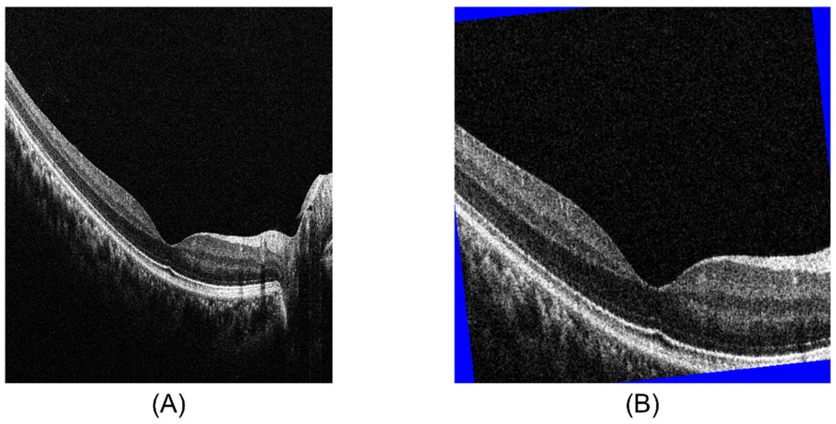
3.1.1. Preprocessing

The ellipsoid zone (EZ), the inner/outer segment of photoreceptors (IS/OS), is the second hyper-reflective band on an OCT image [25,26]. The EZ illuminance in OCT images is reduced when ocular diseases impair photoreceptor cells [27,28]. Thus, EZ luminance is an indicator to diagnose retinal disease in the OCT images. However, the single-shot OCT images contain images in which the boundaries between the interdigitation zone (IZ), EZ, and external limiting membrane (ELM) are challenging to determine. Thus, we applied random (probability = 50%) center cropping to 600 × 600 pixels to zoom in on the IZ, EZ, and ELM. Then, the OCT images were resized to 512 × 512 pixels. After resizing, data augmentation was applied to the input images as follows: random brightness from 0.8 to 2.0 times, random contrast from 0.8 to 1.5 times, random rotation within 10 degrees, random horizontal and vertical shift within 50 pixels, and random (probability = 50%) horizontal mirroring. For margins created by image processing, we used padding with blue (red, green, and blue color information of 0, 0, and 255, respectively) to prevent misrecognition (Figure 1).

3.1.2. Network

In the training phase for transfer learning, supervised learning was used where the network model was given training images. The accuracy of the classification measured as the weights of the deep layers were changed. The weights were changed based on the optimization function. In this study we used the Adam optimizer for all CNN models [29]. The layers of deep neural networks were frozen until just before the output layer in order to use the ImageNet weight parameters. We created the fully connected layer as an output layer. The fully connected layer provided two outputs (abnormal or normal eyes) using the softmax function. We defined an abnormal eye as a predicted value ≥ 0.5.

All CNN models were trained with 2000 epochs. The optimizer used an adaptive learning rate; the primary learning rate was 0.02, which was subsequently reduced to 0.5 times at 25%, 50%, 75%, and 90% of the total number of epochs. The training data were divided into three parts and cross-validated.

We used Python 3.8.5 for Windows 10 (Microsoft Co., Ltd., Redmond, WA, USA), with the following libraries: Matplotlib 3.3.2, Numpy 1.18.5, OpenCV 3.3.1, Pandas 1.1.3, Pytorch 1.7.0, Torchvision 0.8.1, Scikit-learn 0.23.2, and Seaborn 0.11.0.

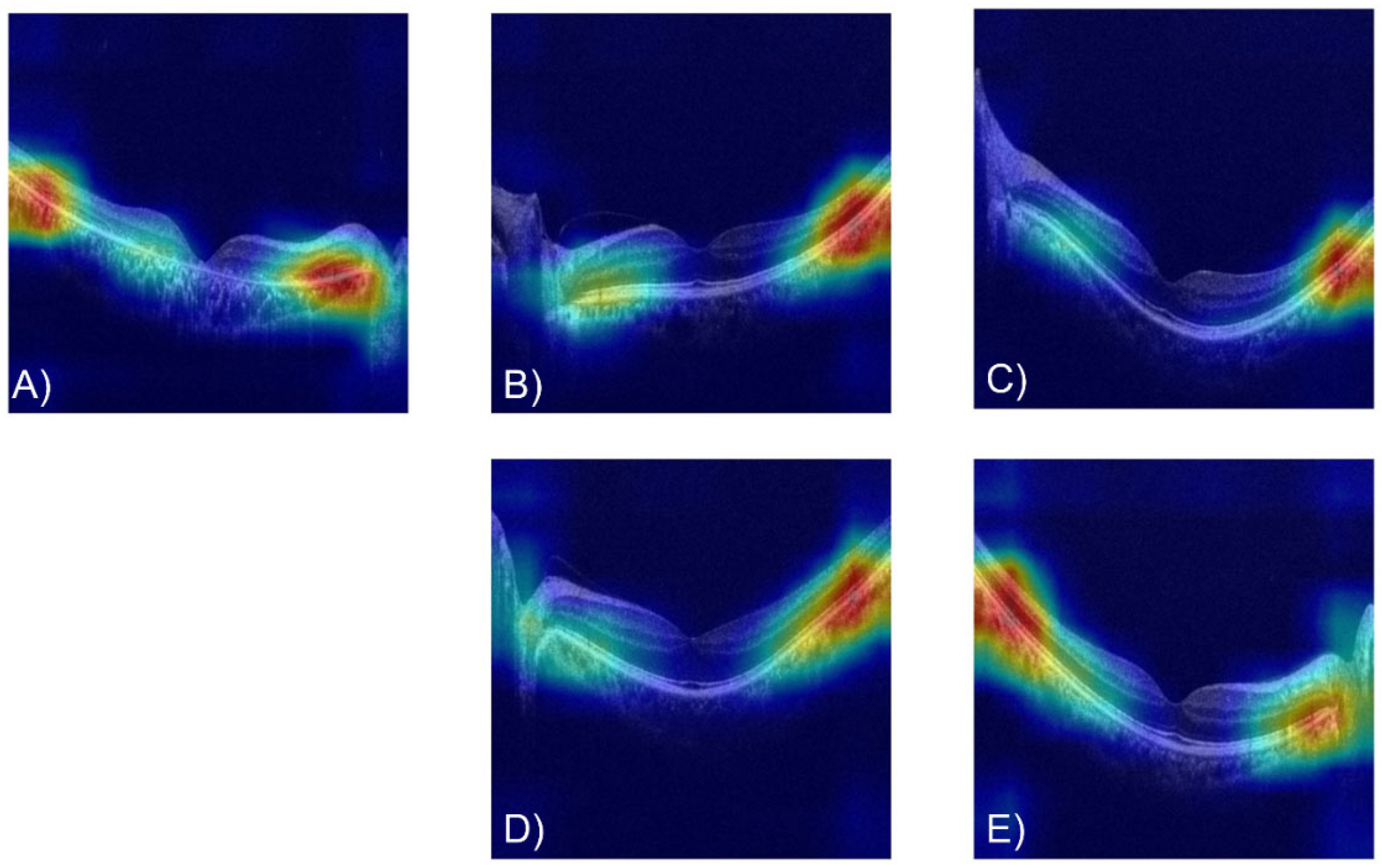
3.1.3. Data Visualization

The explanations for the abnormal predictions by the CNN models were visualized using gradient-weight class activation mapping (Grad-CAM) [30]. Grad-CAM can generate visual explanations from any CNN-based network without requiring architectural changes or retraining. Grad-CAM images were generated using the feature map in the last convolutional layer.

3.1.4. Classification of Ocular Disease

To determine for which diseases the model performed well and poorly, two ophthalmologists (S.U. and T.I.) checked the OCT images in the test data. In cases of multiple ocular diseases, the ocular disease with the most abnormalities was diagnosed.

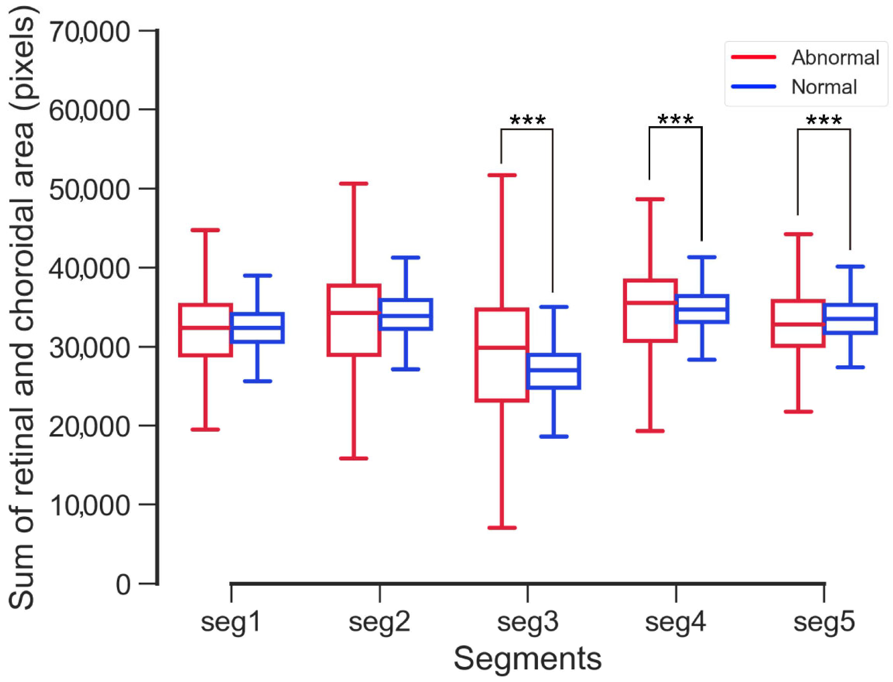
3.1.5. Statistical Analysis

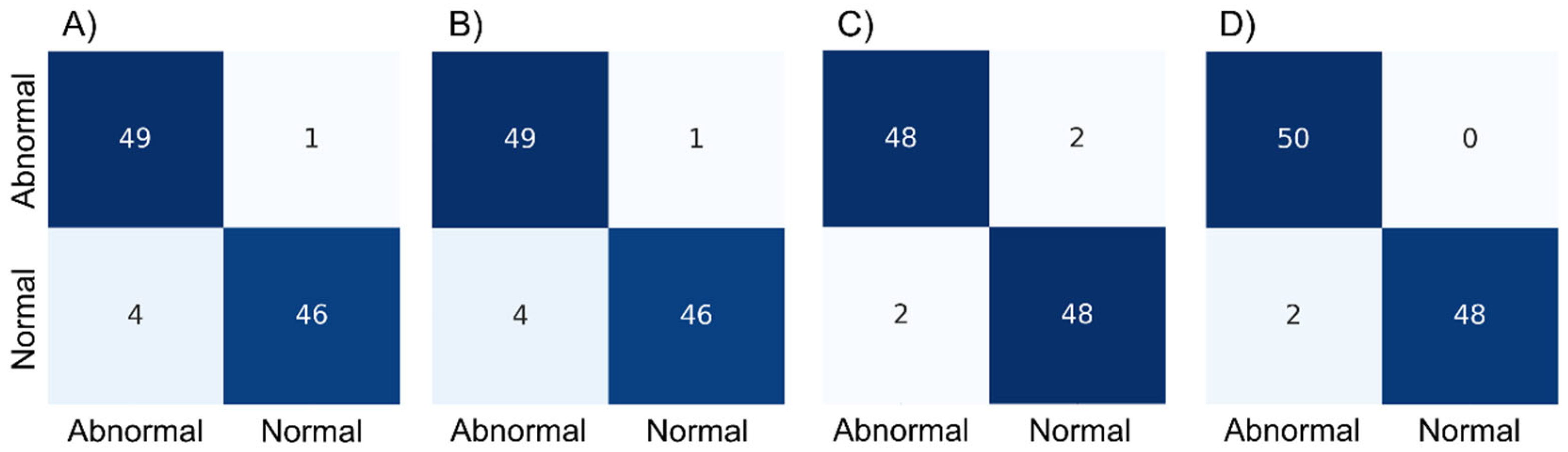
We used receiver-operating characteristic (ROC) curves and calculated the corresponding area under each curve with 1000 times bootstrap to evaluate the screening performance of the CNN and ensemble models. Then, the area under the ROC curve (AUC) was compared among the models using the Scheffé test.

IBM SPSS Statistics version 26 (IBM Corp., Armonk, NY, USA) was used for statistical analysis, and a p-value of <0.05 was considered significant.

3.2. Results 1

Table 1. Detailed overview of the abnormal OCT images.

Disease	Test Data	ResNet Failure	DenseNet Failure	EfficientNet Failure
AMD	5	1
CSC	1
ERM	6			1
Macular edema	14
Macular hole	3
High myopia	5
Post-operation	2
RP	12		1	1
RRD	1
VMTS	1
Total	50	1	1

AMD, age-related macular degeneration; CSC, central serious chorioretinopathy; ERM, epiretinal membrane; OCT, optical coherence tomography; RP, retinitis pigmentosa; RRD, rhegmatogenous retinal detachment; VMTS, vitreomacular traction syndrome.

showed the abnormal OCT images in the test dataset.

The accuracies of the CNN models with ResNet-152, DenseNet-201, and EfficientNet-B7, and the ensemble model were 95.0% (abnormal 49/50, normal 46/50), 95.0% (abnormal 49/50, normal 46/50), 96.0% (abnormal 48/50, normal 48/50), and 98.0% (abnormal 50/50, normal 48/50), respectively (Figure 2). The AUCs of the CNN models with ResNet-152, DenseNet-201, and EfficientNet-B7, and the ensemble model were 0.989 (95% confidence interval [CI], 0.968–1.000), 0.997 (95% CI, 0.986–1.000), 0.997 (95% CI, 0.986–1.000), and 0.998 (95% CI, 0.989–1.000), respectively (Figure 3). Although, the screening performance between each model did not significantly differ, the screening performance in the ensemble model was the highest among the four models.

In most cases, the CNN models focused on abnormal images of the retina to predict the disease (Figure 4). The images that the CNN models misjudged did not have remarkable lesions in the inner retinal layers, and in such cases, the CNN models focused on the nasal and temporal retinal regions to make decisions (Figure 5).

ResNet-152 and DenseNet-201 made incorrect classifications for 5/100 images. EfficientNet-B7 was incorrect for 4/100 images. The ensemble model was incorrect for 2/100 images.

4. Experiment 2

In Experiment 2, we examined the ability of another ML model to identify anomalies in the thickness of peripheral nasal and temporal retinal regions, which was the weak point of the CNN models created in Experiment 1. Then, we developed an ensemble model combining the CNN models (ResNet-152, DenseNet-201, and EfficientNet-B7) and the ML model and verified the screening accuracy.

4.1. Methods

4.1.1. Preprocessing

Twenty percent of the total pixel size of all original OCT images (Figure 6A) was removed from the right and left edges to avoid depression of the optic disc (Resolution: 615 × 1176 pixels; Figure 6B). The OCT images were divided into five sections (Resolution: 123 × 1176 pixels; Figure 6C): the peripheral temporal retina, temporal perimacular area, central macular area, nasal perimacular area, and peripheral nasal retina as segments were defined as segments 1, 2, 3, 4, and 5, respectively. Each section was binarized using the discriminant analysis method (Figure 6D). Morphological closing was applied to these segment images to pad the dark area related to the inner retinal layer and choroidal vessels. The sum of the retinal and choroidal areas (Figure 6E) was then calculated, and the area (in pixels) of each section was exported to an Excel file (Microsoft Co., Ltd., Redmond, WA, USA).

4.1.2. Network

The random forest algorithm was used in Experiment 2 [31]. The random forest algorithm is an ensemble learning method based on bagging. The input data were sampled randomly using bootstrap and divided into multiple groups. Each group was trained using the same decision trees to make them parallel, but this can lead to overfitting. We then averaged the prediction values in each group to prevent overfitting. Data on the retinal and choroidal areas were divided into 100 groups. The depth of the decision trees was set to 5.

Then, the ensemble model was made using a soft-voting algorithm between the CNN models with ResNet-152, DenseNet-201, EfficientNet-B7, and random forest model.

4.1.3. Statistical Analysis

We determined the differences in the retinal and choroidal areas between the abnormal and normal images using the Mann–Whitney U test with Bonferroni correction for each segment. [32]

We used ROC curves and calculated the AUC with 1000 times bootstrap to estimate the screening performance of the random forests, ensemble with CNNs, and ensemble with CNNs and random forest models.

IBM SPSS Statistics version 26 (IBM Corp., Armonk, NY, USA) was used for statistical analysis, and a p-value of <0.05 was considered significant.

4.2. Results

The sum of the retinal and choroidal areas was significantly thicker in the abnormal eyes than in the normal eyes in segments 3 and 4 (p < 0.001) and was significantly thinner in the abnormal eyes than in the normal eyes in segment 5 (p < 0.001; Figure 7). The accuracies of each segment as evaluated by the random forest model were 83% for segment 1 (abnormal 47/50, normal 36/50; Figure 8A), 87% for segment 2 (abnormal 48/50, normal 39/50; Figure 8B), 96% for segment 3 (abnormal 50/50, normal 46/50; Figure 8C), 88% for segment 4 (abnormal 47/50, normal 41/50; Figure 8D), and 89% for segment 5 (abnormal 45/50, normal 44/50; Figure 8E).

The random forests, ensemble with CNNs, and ensemble with CNNs and random forest models showed accuracies of 89% (abnormal 45/50, normal 44/50;

Table 2. Failure data in the random forest model.

Disease	Test Data	Random Forest Failure
AMD	5
CSC	1
ERM	6	1
Macular edema	14	2
Macular hole	3
High myopia	5
Post-operation	2
RP	12	2
RRD	1
VMTS	1
Total	50	5

AMD, age-related macular degeneration; CSC, central serious chorioretinopathy; ERM, epiretinal membrane; OCT, optical coherence tomography; RP, retinitis pigmentosa; RRD, rhegmatogenous retinal detachment; VMTS, vitreomacular traction syndrome.

), 98.0% (abnormal 50/50, normal 48/50), and 99% (abnormal 50/50, normal 49/50), respectively (Figure 9). The screening performances of the random forests, ensemble with CNNs, and ensemble with CNNs and random forest models were 0.962 (95% confidence interval [CI], 0.922–1.000), 0.998 (95% CI, 0.989–1.000), and 0.999 (95% CI, 0.996–1.000), respectively (Figure 10).

The random forest model prediction was unsuccessful when the retinal and choroidal areas were underestimated during image processing (Figure 11). The ensemble with the CNNs and random forest model analyzed 0.025 image/s.

5. Discussion

This study investigated the screening performances of ML models using OCT images obtained from actual eye checkups. The CNN models focused on the structural changes in the retina in abnormal eyes, with accuracy from 95% to 96%, and the screening performance did not differ between each model (Figure 2, Figure 3 and Figure 4). Our finding is consistent with earlier studies that reported a classification accuracy of a single-CNN model of about 70–95%; this model may also miss some diseases using OCT images [10,11,13,14,15]. Furthermore, our findings support the earlier study that the latest CNN model is not necessarily better when performing transfer learning using OCT images [20]. We have considered that the number of classification categories relates to our findings. We developed CNN models for the classification of two categories (abnormal, normal), but did not develop CNN models for the classification of every disease in this study. The binary classification is the simplest classifier in CNN models. Therefore, we expect the differences between CNN models to be more significant for multi-class classifications, such as those for classifying individual retinal diseases.

RP was false-negatively predicted, suggesting insufficient training with abnormalities in the retinal pigment epithelium and photoreceptor layer, including interdigitation and ellipsoid zones in the ELM. In cases with no apparent edema in the inner retinal layer, our CNN models tended to predict an abnormality based on the peripheral temporal and nasal retinal shapes (Figure 5). Russakoff et al. [33] described CNN models trained with OCT images of age-related macular degeneration that focused on the temporal and nasal retinas, and differentiated between progressors and non-progressors. These findings suggest that CNN can detect subtle differences in the morphology of the peripheral temporal and nasal retinal regions, and can therefore differentiate between abnormal and normal eyes or between progressors and non-progressors.

The random forest model used the central macular (segment 3) and nasal (segments 4 and 5) areas as bases for determining eye abnormalities, as a significant difference was found between abnormal and normal retinal areas in both segments (Figure 7 and Figure 8). Of the five diseases that were misjudged by the random forest model (Figure 9A), the retinal and choroidal areas were underestimated because the morphological transformation did not fill in the inner retinal layer with white in ERM (Figure 11A,A′) and macular edema (Figure 11B,B′,C,C′). Furthermore, the OCT images of RP had small retinal and choroidal areas (Figure 11D,D′,E,E′). Most diseases were correctly classified by the random forest model, although cases with an underestimated macular area were misclassified. Therefore, the features of the retinal and choroidal areas extracted by dividing the OCT images into five segments were useful.

The ensemble model had better screening performance than the single-CNN models (Figure 2 and Figure 3). However, the risk of misjudging normal features as abnormal remains. The ensemble with the CNN and random forest model improved that risk. The random forest model, which evaluated for disease using the nasal retinal area, thereby improving on CNN models that misrecognized the nasal peripheral retinal structures (Figure 5 and Figure 7). Thus, the ensemble model combining the CNN models trained with OCT images and the random forest model trained in the retinal area can vastly improve disease prediction during an actual eye or health checkup in which only OCT images are acquired. Furthermore, the ensemble with the CNN and random forest model may be useful to clinicians, given its screening accuracy of 0.999 at 0.025 image/s.

In this study, the ensemble model showed high screening performance in the single-shot OCT images captured during the actual eye checkups, because the random forest model complements the weaknesses of CNN. These findings suggest that our ensemble model can screen for retinal diseases without requiring retakes in the actual eye checkups. On the other hand, we have been concerned that the screening performance will be degraded when our ensemble model is applied for actual in-person eye checkups because we excluded OCT images in which the ophthalmologists had difficulty determining the disease by reading the images alone. Therefore, the accuracy of our ensemble model during actual eye checkups will need to be confirmed in a future investigation.

References

1. Thapa, R.; Khanal, S.; Tan, H.S.; Thapa, S.S.; van Rens, G. Prevalence, Pattern and Risk Factors of Retinal Diseases among an Elderly Population in Nepal: The Bhaktapur Retina Study. Clin. Ophthalmol. 2020, 14, 2109–2118. [Google Scholar] [CrossRef]
2. Klein, R.; Klein, B.E.K. The Prevalence of Age-Related Eye Diseases and Visual Impairment in Aging: Current Estimates. Investig. Opthalmol. Vis. Sci. 2013, 54, ORSF5. [Google Scholar] [CrossRef] [PubMed] [Green Version]
3. Roberts, C.B. Economic Cost of Visual Impairment in Japan. Arch. Ophthalmol. 2010, 128, 766. [Google Scholar] [CrossRef] [PubMed] [Green Version]
4. Hiratsuka, Y.; Ono, K.; Nakano, T.; Tamura, H.; Goto, R.; Kawasaki, R.; Kawashima, M.; Yamada, M. Current status of eye examinations for adults and local government initiatives. J. Jpn. Ophthalmol. Assoc. 2017, 88, 3–22. [Google Scholar]
5. Huang, D.; Swanson, E.A.; Lin, C.P.; Schuman, J.S.; Stinson, W.G.; Chang, W.; Hee, M.R.; Flotte, T.; Gregory, K.; Puliafito, C.A.; et al. Optical Coherence Tomography. Science 1991, 254, 1178–1181. [Google Scholar] [CrossRef] [Green Version]
6. Jaffe, G.J.; Caprioli, J. Optical coherence tomography to detect and manage retinal disease and glaucoma. Am. J. Ophthalmol. 2004, 137, 156–169. [Google Scholar] [CrossRef]
7. Gibson, D.M. The geographic distribution of eye care providers in the United States: Implications for a national strategy to improve vision health. Prev. Med. 2015, 73, 30–36. [Google Scholar] [CrossRef]
8. Center for Disease Control and Prevention. National Diabetes Statistics Report 2020. Available online: https://www.cdc.gov/diabetes/pdfs/data/statistics/national-diabetes-statistics-report.pdf (accessed on 28 May 2022).
9. Krizhevsky, A.; Sutskever, I.; Hinton, G.E. ImageNet Classification with Deep Convolutional Neural Networks. Commun. ACM 2017, 60, 84–90. [Google Scholar] [CrossRef]
10. Lee, C.S.; Baughman, D.M.; Lee, A.Y. Deep Learning Is Effective for Classifying Normal versus Age-Related Macular Degeneration OCT Images. Ophthalmol. Retin. 2017, 1, 322–327. [Google Scholar] [CrossRef]
11. Yoon, J.; Han, J.; Park, J.I.; Hwang, J.S.; Han, J.M.; Sohn, J.; Park, K.H.; Hwang, D.D.-J. Optical coherence tomography-based deep-learning model for detecting central serous chorioretinopathy. Sci. Rep. 2020, 10, 18852. [Google Scholar] [CrossRef]
12. De Fauw, J.; Ledsam, J.R.; Romera-Paredes, B.; Nikolov, S.; Tomasev, N.; Blackwell, S.; Askham, H.; Glorot, X.; O’Donoghue, B.; Visentin, D.; et al. Clinically applicable deep learning for diagnosis and referral in retinal disease. Nat. Med. 2018, 24, 1342–1350. [Google Scholar] [CrossRef]
13. Yoo, T.K.; Choi, J.Y.; Seo, J.G.; Ramasubramanian, B.; Selvaperumal, S.; Kim, D.W. The possibility of the combination of OCT and fundus images for improving the diagnostic accuracy of deep learning for age-related macular degeneration: A preliminary experiment. Med. Biol. Eng. Comput. 2019, 57, 677–687. [Google Scholar] [CrossRef] [PubMed]
14. Awais, M.; Müller, H.; Tang, T.B.; Meriaudeau, F. Classification of SD-OCT images using a Deep learning approach. In Proceedings of the 2017 IEEE International Conference on Signal and Image Processing Applications (ICSIPA), Kuching, Malaysia, 12–14 September 2017; pp. 489–492. [Google Scholar]
15. Wang, J.; Deng, G.; Li, W.; Chen, Y.; Gao, F.; Liu, H.; He, Y.; Shi, G. Deep learning for quality assessment of retinal OCT images. Biomed. Opt. Express 2019, 10, 6057–6072. [Google Scholar] [CrossRef] [PubMed]
16. He, K.; Zhang, X.; Ren, S.; Sun, J. Deep Residual Learning for Image Recognition. arXiv 2015, arXiv:1512.03385. [Google Scholar]
17. Simonyan, K.; Zisserman, A. Very Deep Convolutional Networks for Large-Scale Image Recognition. arXiv 2015, arXiv:1409.1556. [Google Scholar]
18. Huang, G.; Liu, Z.; van der Maaten, L.; Weinberger, K.Q. Densely Connected Convolutional Networks. arXiv 2018, arXiv:1608.06993v5. [Google Scholar]
19. Tan, M.; Quoc. EfficientNet: Rethinking Model Scaling for Convolutional Neural Networks. arXiv 2020, arXiv:1905.11946. [Google Scholar]
20. Roy, K.; Chaudhuri, S.S.; Roy, P.; Chatterjee, S.; Banerjee, S. Transfer Learning Coupled Convolution Neural Networks in Detecting Retinal Diseases Using OCT Images. In Intelligent Computing: Image Processing Based Applications; Mandal, J., Banerjee, S., Eds.; Springer: Singapore, 2020; Volume 1157, pp. 153–173. [Google Scholar]
21. Van Der Heijden, A.A.; Abramoff, M.D.; Verbraak, F.; Van Hecke, M.V.; Liem, A.; Nijpels, G. Validation of automated screening for referable diabetic retinopathy with the IDx-DR device in the Hoorn Diabetes Care System. Acta Ophthalmol. 2018, 96, 63–68. [Google Scholar] [CrossRef]
22. Abràmoff, M.D.; Lavin, P.T.; Birch, M.; Shah, N.; Folk, J.C. Pivotal trial of an autonomous AI-based diagnostic system for detection of diabetic retinopathy in primary care offices. NPJ Digit. Med. 2018, 1, 39. [Google Scholar] [CrossRef]
23. Ovadia, Y.; Fertig, E.; Ren, J.; Nado, Z.; Sculley, D.; Nowozin, S.; Dillon, J.V.; Lakshminarayanan, B.; Snoek, J. Can You Trust Your Model’s Uncertainty? Evaluating Predictive Uncertainty Under Dataset Shift. arXiv 2019, arXiv:1906.02530. [Google Scholar]
24. Tufail, A.; Kapetanakis, V.V.; Salas-Vega, S.; Egan, C.; Rudisill, C.; Owen, C.G.; Lee, A.; Louw, V.; Anderson, J.; Liew, G.; et al. An observational study to assess if automated diabetic retinopathy image assessment software can replace one or more steps of manual imaging grading and to determine their cost-effectiveness. Health Technol. Assess. 2016, 20, 1–72. [Google Scholar] [CrossRef] [PubMed] [Green Version]
25. Wu, Z.; Ayton, L.N.; Guymer, R.H.; Luu, C.D. Second reflective band intensity in age-related macular degeneration. Ophthalmology 2013, 120, 1307–1308.e1. [Google Scholar] [CrossRef] [PubMed]
26. Tao, L.W.; Wu, Z.; Guymer, R.H.; Luu, C.D. Ellipsoid zone on optical coherence tomography: A review. Clin. Exp. Ophthalmol. 2016, 44, 422–430. [Google Scholar] [CrossRef]
27. Wu, Z.; Ayton, L.N.; Guymer, R.H.; Luu, C.D. Relationship Between the Second Reflective Band on Optical Coherence Tomography and Multifocal Electroretinography in Age-Related Macular Degeneration. Investig. Opthalmol. Vis. Sci. 2013, 54, 2800. [Google Scholar] [CrossRef] [PubMed] [Green Version]
28. Gomes, N.L.; Greenstein, V.C.; Carlson, J.N.; Tsang, S.H.; Smith, R.T.; Carr, R.E.; Hood, D.C.; Chang, S. A Comparison of Fundus Autofluorescence and Retinal Structure in Patients with Stargardt Disease. Investig. Opthalmol. Vis. Sci. 2009, 50, 3953. [Google Scholar] [CrossRef] [PubMed] [Green Version]
29. Kingma, D.P.; Ba, J.L. Adam: A Method for Stochastic Optimization. arXiv 2017, arXiv:1412.6980. [Google Scholar]
30. Selvaraju, R.; Cogswell, M.; Das, A.; Vedantam, R.; Parikh, D.; Batra, D. Grad-CAM: Visual Explanations from Deep Networks via Gradient-based Localization. arXiv 2017, arXiv:1610.02391v02393. [Google Scholar]
31. Louppe, G. Understanding Random Forests: From Theory to Practice. arXiv 2015, arXiv:1407.7502. [Google Scholar]
32. Ranstam, J. Multiple p-values and Bonferroni correction. Osteoarthr. Cartil. 2016, 24, 763–764. [Google Scholar] [CrossRef] [Green Version]
33. Russakoff, D.B.; Lamin, A.; Oakley, J.D.; Dubis, A.M.; Sivaprasad, S. Deep Learning for Prediction of AMD Progression: A Pilot Study. Investig. Opthalmol. Vis. Sci. 2019, 60, 712. [Google Scholar] [CrossRef] [Green Version]
Figure 1. Data augmentation for training the CNN model. Original OCT image (A) with a resolution of 1021 × 1176 pixels was center-cropped to 600 × 600 pixels (probability = 50%) and then resized to 512 × 512 pixels. After resizing, the following data augmentations were applied to the images: random brightness from 0.8 to 2.0 times, random contrast from 0.8 to 1.5 times, random rotation within 10 degrees, random horizontal and vertical shift within 50 pixels, and random horizontal mirroring (probability = 50%). (B) If margins were created by image processing, these were padded with blue (red, green, and blue color information of 0, 0, and 255, respectively) to prevent misrecognition. Abbreviations: CNN, convolutional neural network; OCT, optical coherence tomography.
Applsci 12 06872 g001
Figure 2. Confusion matrix in the (A) ResNet-152, (B) DenseNet-201, (C) EfficientNet-B7, and (D) ensemble models. The horizontal and vertical labels indicate the prediction by each model and ground truth, respectively. (A) ResNet-152 showed an accuracy of 95% (abnormal 49/50, normal 46/50). (B) DenseNet-201 showed an accuracy of 95% (abnormal 49/50, normal 46/50). (C) EfficientNet-B7 showed an accuracy of 96% (abnormal 48/50, normal 48/50). (D) The ensemble model showed an accuracy of 99% (abnormal 50/50, normal 48/50).
Applsci 12 06872 g002
Figure 3. Diagnostic performances of the ResNet-152 (green), DenseNet-201 (purple), EfficientNet-B7 (blue), and ensemble models (red). The diagnostic performances of the CNN model with ResNet-152, DenseNet-201, and EfficientNet-B7 and the ensemble model were 0.989 (95% CI, 0.968–1.000), 0.997 (95% CI, 0.986–1.000), 0.997 (95% CI, 0.986–1.000), and 0.998 (95% CI, 0.989–1.000), respectively. The diagnostic performance was significantly greater in the ensemble model than in the other CNN models (p < 0.001). Abbreviations: CNN, convolutional neural network; CI, confidence interval.
Applsci 12 06872 g003
Figure 4. Representative visual explanations of the feature map of the CNN model in the corrected OCT image. The heat maps in (A) macular hole, (B) macular edema, and (C) epiretinal membrane indicate the relative activation intensity of predicting abnormalities in the OCT images. Warm colors indicate areas of high attention for classification. The CNN model made a decision based on the location of the warm color. The CNN model focused on the retinal structural changes in the abnormal eyes. Abbreviations: OCT, optical coherence tomography; CNN, convolutional neural network.
Applsci 12 06872 g004
Figure 5. Representative visual explanations of the feature map of the CNN model in the misrecognized OCT images. The heat maps in (AE) indicate the relative activation intensity of predicting abnormalities in OCT images. The CNN model made a decision based on the location of the warm color. The CNN model classified (A) an abnormal eye (retinitis pigmentosa) as normal and (BE) a normal eye as abnormal.
Applsci 12 06872 g005
Figure 6. All original OCT images (A) had 20% of pixels removed from the right and left edges (red line and red arrows) to avoid (B) depression of the optic disk. (C) The OCT images were divided into five sections, each with a resolution of 123 × 1176 pixels. The peripheral temporal retina, temporal perimacular area, central macular area, nasal perimacular area, and peripheral nasal retina were defined as segments 1, 2, 3, 4, and 5, respectively. (D) Each section was binarized using the discriminant analysis method. (E) Morphological closing was applied to these segment images to pad the dark area related to the inner retinal layer and choroidal vessels. The sum of the retinal and choroidal areas was then calculated. Abbreviations: OCT, optical coherence tomography; ML, machine learning; seg, segment.
Applsci 12 06872 g006
Figure 7. Sum of the retinal and choroidal areas in each segment. The peripheral temporal retina, temporal perimacular area, central macular area, nasal perimacular area, and peripheral nasal retina were defined as segments 1, 2, 3, 4, and 5, respectively. The sum of the retinal and choroidal areas was significantly thicker in abnormal eyes than in normal eyes in segments 3 and 4. Furthermore, the retinal and choroidal areas were significantly thinner in abnormal eyes than in normal eyes in segment 5. Abbreviation: seg, segment. *** p < 0.001.
Applsci 12 06872 g007
Figure 8. Classification of each segment in the ML model. The red and green dots and areas indicate the abnormal and normal eyes classified by the ML model in each segment. The accuracies of each segment were (A) 83% for segment 1 (peripheral temporal retina), (B) 87% for segment 2 (temporal perimacular area), (C) 96% for segment 3 (central macular area), (D) 88% for segment 4 (nasal perimacular area), and (E) 89% for segment 5 (peripheral nasal retina). Abbreviation: ML, machine learning.
Applsci 12 06872 g008
Figure 9. Confusion matrix in the (A) ML, (B) ensemble with CNNs, and (C) ensemble with CNNs and ML models. The horizontal and vertical labels indicate the prediction by each model and ground truth, respectively. (A) The ML model showed an accuracy of 89% (abnormal 45/50, normal 44/50). (B) The ensemble model with three CNN models showed accuracies of 98.0% (abnormal 50/50, normal 48/50) and 99% (abnormal 50/50, normal 49/50). (C) The ensemble with three CNNs and ML models showed an accuracy of 99% (abnormal 50/50, normal 49/50). Abbreviation: ML, machine learning.
Applsci 12 06872 g009
Figure 10. Diagnostic performances of the ML (purple), ensemble (blue), and ensemble with ML (red) models. The diagnostic performances of the ML, ensemble, and ensemble with ML models were 0.962 (95% CI, 0.922–1.000), 0.998 (95% CI, 0.989–1.000), and 0.999 (95% CI, 0.996–1.000), respectively. The diagnostic performance was significantly greater in the ensemble model with ML than in both ML and ensemble models (p < 0.001). Abbreviations: ML, machine learning; CI, confidence interval.
Applsci 12 06872 g010
Figure 11. Original (AE) and post-processing (A′–E′) OCT images misjudged by the ML model. The ML model misinterpreted epiretinal membrane (A), macular edema (B,C), and retinitis pigmentosa (D,E). In the OCT images of the epiretinal membrane and macular edema, the inner retinal layer was not filled in with white by morphological transformation. The OCT images of retinitis pigmentosa indicate small retinal and choroidal areas. Abbreviations: OCT, optical coherence tomography; ML, machine learning.
Applsci 12 06872 g011