Dynamic Analysis of the Musical Triangles—Experimental and Numerical Approaches

Abstract

This paper addresses the experimental and numerical dynamic analysis of curved bars used as percussion musical instruments. These structures are known as triangles, being made of various metal materials. The study was based on the experimental analysis of the dynamic response over time and the frequency of three types of triangles, different in material and size. Subsequently, finite element analysis of the same structures modeled with the SimCenter 12 program was performed. The results were compared, highlighting the contribution of material type and geometry in obtaining vibration modes, frequency spectrum, and structural damping coefficient. Between the experimental and the numerical analysis, the obtained errors were below 2.2% in terms of their natural frequencies. The study also highlights the complementarity of the two methods in understanding the vibration modes of triangles.

1. Introduction

The history of musical instruments is intertwined with anthropological evolution, from the most rudimentary sound-generating forms and structures to the most evolved current musical systems.

The materials used in the structure of musical instruments are varied both in terms of chemistry, the old–new timeframe, and the elastic, mechanical, and strength characteristics of the components in the structure of musical instruments. Thus, there are natural materials—metals, wood, leather, hair, bones and ivory, plants, and natural fibers (linen, silk, hemp, wool), as well as synthetic materials—nylon, carbon fiber, artificial silk, polymers, and so on. The use of traditional materials in combination with modern ones aims to increase the reliability and quality of musical instruments by maintaining over time both their acoustic and aesthetic quality and their mechanical strength to different types of stresses.

According to the way in which air vibration is generated for the production of sounds, there are five categories of musical instruments: brass and woodwind instruments, idiophone instruments, chordophone instruments, instruments with vibrating diaphragm, and electro–acoustic instruments (Figure 1).

The triangle is an idiophone musical instrument consisting of a metal bar bent in the form of an equilateral or isosceles open triangle, with rounded tips, the sound being produced only by vibrating its own body, without the use of any auxiliary part.

The triangle has a very crystalline sound, which mimics bells. Unlike the timpani, the small drum, the marimba, or the xylophone, the triangle is not a solo instrument, but appears in symphonies, overtures, or concerts in the form of short signals or tremolo [1,2]. The acoustic quality of the sounds emitted by the triangle depends on the material from which it is made [3,4,5,6]. Triangles are made of a bent metal alloy rod (steel, aluminum, copper), produced by folding the metal around a template. Their section is generally circular and constant along the entire length of the bar, but there are also variants with variable thickness. Its shape can be an equilateral or isosceles triangle. The triangle has several shapes and sizes: most are 5 inches, but can also be 6.7 or 8 inches. The sound is directly influenced by its size, the larger ones having louder sounds, but more serious tones due to differences in vibration. The smaller ones have higher tones, but lower amplitudes of vibrations. In order for the sound to be able to produce and pass on the harmonics, the triangle is not closed [7,8,9].

The orchestral triangle is actually a combination of straight and curved bars, so it is an instrument with a relatively complex structure [4,6,10,11]. To emit musical sounds, the triangle is struck with a metal rod on one side and supported by an elastic thread in the upper corner of the suspended instrument. The rods used to strike the triangle are of different thicknesses and the tip may differ in size and thickness. The choice of these sticks is made according to the size and thickness of the rod, which in turn is chosen according to the requirements of the score. Depending on the writing and the character of the work, of course, the way the sound is produced also changes. In short signals, the triangle is held suspended on the support and hit with a wand on one of the three sides.

If you want to obtain short sounds, the vibration of the triangle is stopped by touching (plugging) it with your hand immediately after the sound is produced; however, if the intervention of the triangle is in a more expressive, delicate moment, and the duration of the sounds he has to interpret is longer, the percussionist will hold the triangle with his left hand, will operate the instrument with the wand on one of the three sides, and with his left hand he will move the triangle to produce the vibrato effect [2,3,4,5].

In the music literature, the triangle also appears in the form of thematic signals, in dialogue with solo instruments, as it is in the third part of Concerto No. 1 for piano and orchestra, by Franz Liszt. In this concert, the triangle plays a very important role through its intervention in the form of short, percussive signals, which dialogue directly with the solo instrument, throughout the third part. In fact, Franz Liszt was the first to give the triangle instrument the chance to be a soloist with the piano. Following the performance of this concert, it was called “trianglo concerto”.

Another important effect that the triangle produces is that of tremollo, which is introduced in moments of coral with the wind instruments or in strong dynamic moments, speaking from a musical point of view. The tremollo effect is achieved by the rapid movement of the wand inside the triangle, repeatedly hitting the two closed angles of the instrument [7,8,9,12,13].

The triangle struck on different sides generates longitudinal and bending modes of vibration, which are excited perpendicularly or parallel to the plane of the triangle. The duration of the sound emitted is controlled by the instrumentalist by canceling the vibrations of the triangle by hand or a sound-absorbing material [14,15,16,17]. Both practice and theory show that the elastic characteristics of the triangle material are closely related to the fundamental frequency and the frequency spectrum emitted by the idiophone instrument. For vibrations perpendicular to the plane of the triangle, the displacement is small.

As mentioned [5,7,17], for transverse modes, the vibration modes of a triangle are almost identical to those of the straight bar from which the triangle is bent. This statement supports the hypothesis that the shape of the triangle does not have a large effect on its modes of vibration. However, ref. [14] noted that bending a bar influences the stress distribution, which depends on the moments of inertia that apply to the ends of a bar. For bending vibrations in the plane, there is an important discontinuity in impedance at each bending angle. The transverse vibration inside a side is coupled with the longitudinal vibration on the adjacent side. Therefore, each side of the triangle will have its own vibration modes and will be coupled to another side, to form sets of three own modes, for a side of the same length.

Triangles are usually made of hardened carbon steel or 304 stainless steel, which is non-magnetic and highly resistant to oxidation under atmospheric conditions. High-quality bronze alloys and copper–beryllium alloys are also used, and the sound produced by the triangle is lighter or warmer. The musical triangles used in orchestras are mostly in the shape of a sharp isosceles triangle and vibrate at lower frequencies.

Researchers [7,8,12] analyzed the spectrum of a musical note produced by a struck orchestral triangle and [12,14] analyzed the spectrograms of two triangles with a side of 8 inches (or about 20 cm), considered by musicians to be of high quality and low quality. In contrast, the low-quality triangle has only one dominant frequency [7]. It was also found that the spectrum of the high-quality triangle is characterized by its dominant frequencies, and the damping has a lower value, so the sound persists longer. Previous studies confirm that the geometric aspects of the triangle have a decisive effect on the modes of vibration [11,13,14,15,16].

According to [15,16,17,18,19,20], from a mechanical point of view, the triangle is a combination of straight bars and continuous curved bars. The low-frequency vibration modes are mainly bending and are strictly related to the size and mechanical properties of the material from which the instrument is made. As the side length increases, the fundamental frequency decreases. In previous studies [17], the influence of the size of the sides and angles of the triangle on the dynamic response was analyzed. Thus, the results showed that the size of the angles changes their own frequencies in inverse proportion: with the increase of the peak angle from 30° to 60° and 90°, the eigenvalue decreased in the ratio of 1:1.39:1.611. As the length increases from 200 mm to 450 mm, the value of its own frequency decreases by almost 5.6 times.

Based on the state of the art, it was found that there are only several sporadic studies on the modes of vibration of triangles, usually for commercial ones; these are studies that focused more on finite element modal analysis.

This paper aimed at a dynamic analysis of triangles made of different metallic materials, based on experimental and numerical modal analysis, as a result, deepening the study of the dynamic analysis of triangles from different materials with different dimensions, which is a necessary step in the development of knowledge of this musical instrument.

2. Materials and Methods

2.1. Materials

The study analyzed three types of triangles: a stainless steel triangle, denoted triangle T1, an aluminum alloy triangle, denoted T2, with dimensions close to triangle T1, and an aluminum triangle, T3, with larger dimensions. All three triangles are commercial musical instruments. The differences between the three triangles were the material of the bar and the sizes of the sides. The physical characteristics of the triangles are shown in

Table 1. The physical features of samples.

Type of Triangle	Length of Sides (mm)			Diameter (mm)	Mass (g)	Density (kg/m3)	Materials
	A	B	C
T1	149	161	149	7.84	166.971	2708	Stainless steel
T2	162	170	162	9.60	88.895	7818	Aluminum
T3	214	222.5	214	9.60	118.644	7818	Aluminum

. Each side was denoted by A, B, or C, as seen in Figure 2.

2.2. Methods

2.2.1. Experimental Tests

The test method consisted of hitting the triangles on each side with the impact hammer, thus simulating the actual excitation of the percussion instrument. Triangle signals were recorded by a microphone fixed near the triangle. The sample was supported as well as the grip during the musical performance. The triangle was supported with an elastic element at the node formed by the sides A and B. The experimental setup is presented in Figure 2. Each side was hit three times in succession, and the signals were acquired. These were processed through a program developed in Matlab to determine the time and frequency response of the tested samples.

2.2.2. Numerical Simulation of Forced Vibration

Simcenter 12 software was used for both the geometric model and the modal analysis. Given that the geometric model of the triangle is made in three dimensions, three-dimensional finite elements with four nodes were chosen for discrete analysis, using a tetrahedral shape: CTETRA (4), with a side length of 1 mm, was the value chosen using the time analysis calculation. Thus, the structure was discretized in 1,988,972 finite elements and 38,066 nodes. The solution used in Simcenter 12 to determine its own frequencies and modes was SOL 103 Real Eigenvalues, the solver used was NX Nastran. The first 25 eigenfrequencies (natural frequencies) and the shapes of the corresponding eigenmodes were determined. In general, a modal analysis studies the behavior of a structure in free vibration mode. In the present case, the purpose was to perform an analysis in accordance with the experimental method, where the triangle was attached to a support by means of a connecting element, which did not allow the structure to translate on the x, y, and z axes. In finite element analysis, this was implemented in the boundary condition by blocking translational movements on the three axes of a node in the grip area of the structure, as can be seen in Figure 3.

The engineering constants and the density for the materials of the three triangles were determined experimentally by testing some samples extracted from the triangles using a tensile test, in accordance with [20].

Table 2. The engineering constants of triangle materials.

Type of Triangle	Elasticity Modulus (MPa)	Density (kg/m3)	Poisson Coefficient	Materials
T1	184,479	7818	0.30	Stainless steel
T2	68,382	2708	0.33	Aluminum
T3	68,382	2708	0.33	Aluminum

shows the values of elastic properties used in finite element analysis.

2.2.3. Modal Transient Response Analysis

Transient dynamic response analysis is the most general method of calculating the forced dynamic response. The purpose of such an analysis is to determine the behavior of a structure subjected to an excitation that varies over time [20,21,22,23,24,25]. Transient excitation is explicitly defined in the time domain. All loadings applied to the structure are known at all times, and the results of a transient response analysis are usually displacements, velocities, and accelerations of the points in the model and stresses in the elements. The dynamic analysis in the transient mode was also performed with the Simcenter 12 software; for this type of analysis the SOL 112 Modal Transient Response solution was used [21]. The principle of the method consists of transforming the physical coordinates denoted by $\left\{u\left(t\right)\right\}$ into modal coordinates denoted by $\left\{\xi \left(t\right)\right\}$, assuming that

$$\left\{u\left(t\right)\right\}=\left[\varphi \right]\left\{\xi \left(t\right)\right\},$$

(1)

where $\left[\varphi \right]$ is the mode shapes.

Taking into account the equation of motion $\left\{P\left(t\right)\right\}$ (2) and ignoring temporarily damping, Equation (3) is obtained [21,22,23,24,25]:

$$\left[M\right]\left\{\ddot{u}\left(t\right)\right\}+\left[B\right]\left\{\dot{u}\left(t\right)\right\}+\left[K\right]\left\{u\left(t\right)\right\}=\left\{P\left(t\right)\right\},$$

(2)

$$\left[M\right]\left\{\ddot{u}\left(t\right)\right\}+\left[K\right]\left\{u\left(t\right)\right\}=\left\{P\left(t\right)\right\},$$

(3)

where [M], [B], and [K] are the matrices of mass, viscous damping, and stiffness, respectively.

Replacing in (3) relation (1), results coupled equation of motion (4):

$$\left[M\right]\left[\varphi \right]\left\{\ddot{\xi }\left(t\right)\right\}+\left[K\right]\left[\varphi \right]\left\{\xi \left(t\right)\right\}=\left\{P\left(t\right)\right\},$$

(4)

To uncouple the equation of motion, we multiply Equation (4) by ${\left[\varphi \right]}^T$ to obtain (5):

$${\left[\varphi \right]}^T\left[M\right]\left[\varphi \right]\left\{\ddot{\xi }\right\}+{\left[\varphi \right]}^T\left[K\right]\left[\varphi \right]\left\{\xi \right\}={\left[\varphi \right]}^T\left\{P\left(t\right)\right\},$$

(5)

where ${\left[\varphi \right]}^T\left[M\right]\left[\varphi \right]$ is modal generalized mass matrix; ${\left[\varphi \right]}^T\left[K\right]\left[\varphi \right]$—modal generalized stiffness matrix; ${\left[\varphi \right]}^T\left\{P\left(t\right)\right\}$—modal force vector.

Since the matrices of mass and modal stiffness are diagonal matrices and have no off-diagonal terms, the equations of motion are uncoupled and can be written as a set of systems with a single degree of freedom (6) [21,22,23,24,25]:

$$m_i{\ddot{\xi }}_i\left(t\right)+k_i{\xi }_i\left(t\right)=p_i\left(t\right),$$

(6)

where $m_i$ is the modal mass for the ith mode; $k_i$—modal stiffness for the ith mode; $p_i$—modal force for the ith mode.

Once the individual modal responses, ${\xi }_i\left(t\right),$ are computed, physical responses are recovered as the summation of the modal responses using (7):

$$\left\{u\left(t\right)\right\}=\left[\varphi \right]\left\{\xi \left(t\right)\right\},$$

(7)

In this study, the experimentally determined structural damping was introduced in the transient analysis, taking into account the dominant frequency at which the damping is active [21,22,23,24,25]. Thus, the structural damping is converted to viscous damping and the modal viscous damping matrix $\left[B_{qq}\right]$ is obtained based on relation (8):

$$\left[B_{qq}\right]=\left[{\varphi }_{dq}^T\right]\left(\left[B_{dd}^1\right]+\left[B_{dd}^2\right]+\frac{G}{W_3}\left[K_{dd}^1\right]+\frac{1}{W_4}\left[K_{dd}^4\right]\right)\left[{\varphi }_{dq}\right],$$

(8)

where $\left[{\varphi }_{dq}\right]$ is mode shape matrix; $\left[B_{dd}^1\right]$—assembled viscous damping matrix; $\left[B_{dd}^2\right]$—viscous damping matrix from direct matrix input at points; $\left[K_{dd}^1\right]$—assembled stiffness matrix; $\left[K_{dd}^4\right]$—assembled elemental damping matrix from specifying the element structural damping field on material, property, and element entries; $G$—overall structural damping coefficient; $W_3$—user-defined conversion frequency for overall structural damping; $W_4$—user-defined conversion frequency for elemental structural damping [21].

As input data, in addition to the elastic properties of the materials, the damping factor of the structure was required for this analysis. It was determined experimentally, based on the time response of the structure. An approximate method of determining the value of the depreciation factor is by calculating the logarithmic decrement. This involves the analysis of two consecutive amplitudes in the graph of the response of the structure over time to the dynamic stress, as can be seen in Figure 4.

Thus, the damping factor was calculated for five pairs of consecutive amplitudes using relations (9) and (10) in accordance with [20].

$$\Delta =ln\left(\frac{A_1}{A_2}\right),$$

(9)

$$\xi =\frac{\Delta }{2\pi },$$

(10)

where Δ is the logarithmic decrement, A₁ and A₂—two consecutive amplitudes, and ξ—the damping factor of the structure.

Similar to the experimental method, in numerical analysis, the triangle was excited by applying a force over time. The intensity of this force was correlated with that in the experiment, the value of which was identified when the triangle was struck by the impact hammer. In finite element analysis, the force was applied to the middle of the A side for a time of 0.01 s, having a value of 550 N. The boundary conditions were identical to those imposed for the modal analysis. Two analyses were performed, one for the stainless steel triangle and one for the aluminum triangle, following which the time variation of the node displacement was determined with the maximum displacement value.

3. Results

3.1. Comparison between Experimental and Numerical Modal Analysis

Following the experimental tests, the acquired signals were processed. Thus, the time and frequency response were obtained for each triangle tested (Figure 5a–c). Thus, 54 results were generated and processed from which the natural frequency values were extracted for each type of triangle separately, respectively, for each individual test, the data being centralized in

Table 3. The first natural frequencies obtained experimentally.

Type of Triangle	Excited Side	Average Values of Frequency (Hz)
		f1	f2	f3	f4	fAmax
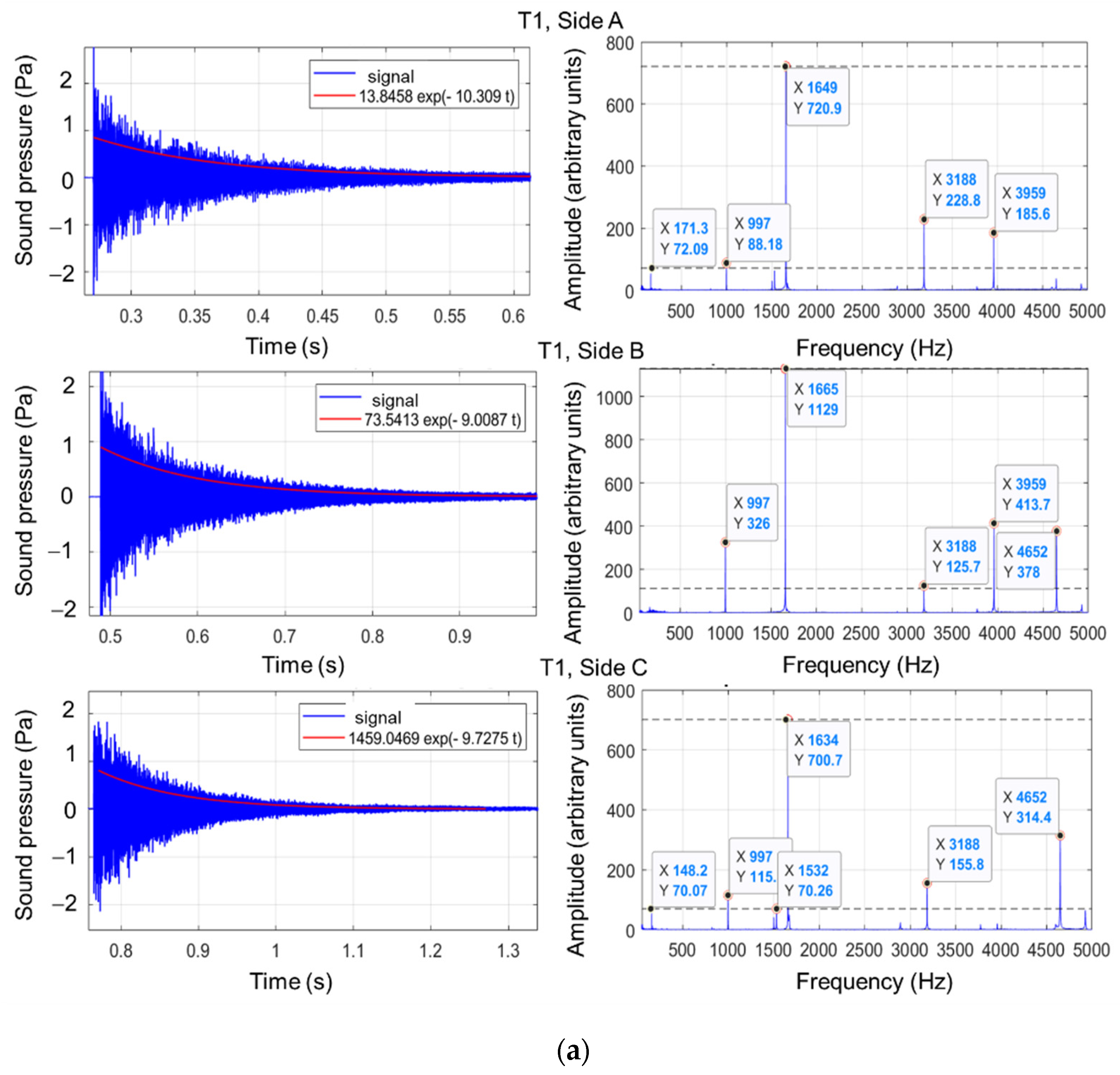
T1	A	159.43	997.30	1531.33	-	1657.10
	B	-	996.97	-	-	1657.10
	C	159.53	996.97	1531.66	-	1657.10
T2	A	168.13	878.13	1053.00	1605.80	1876.06
	B	-	878.10	1052.90	1606.00	1876.29
	C	168.20	878.17	1054.71	1597.66	1876.57
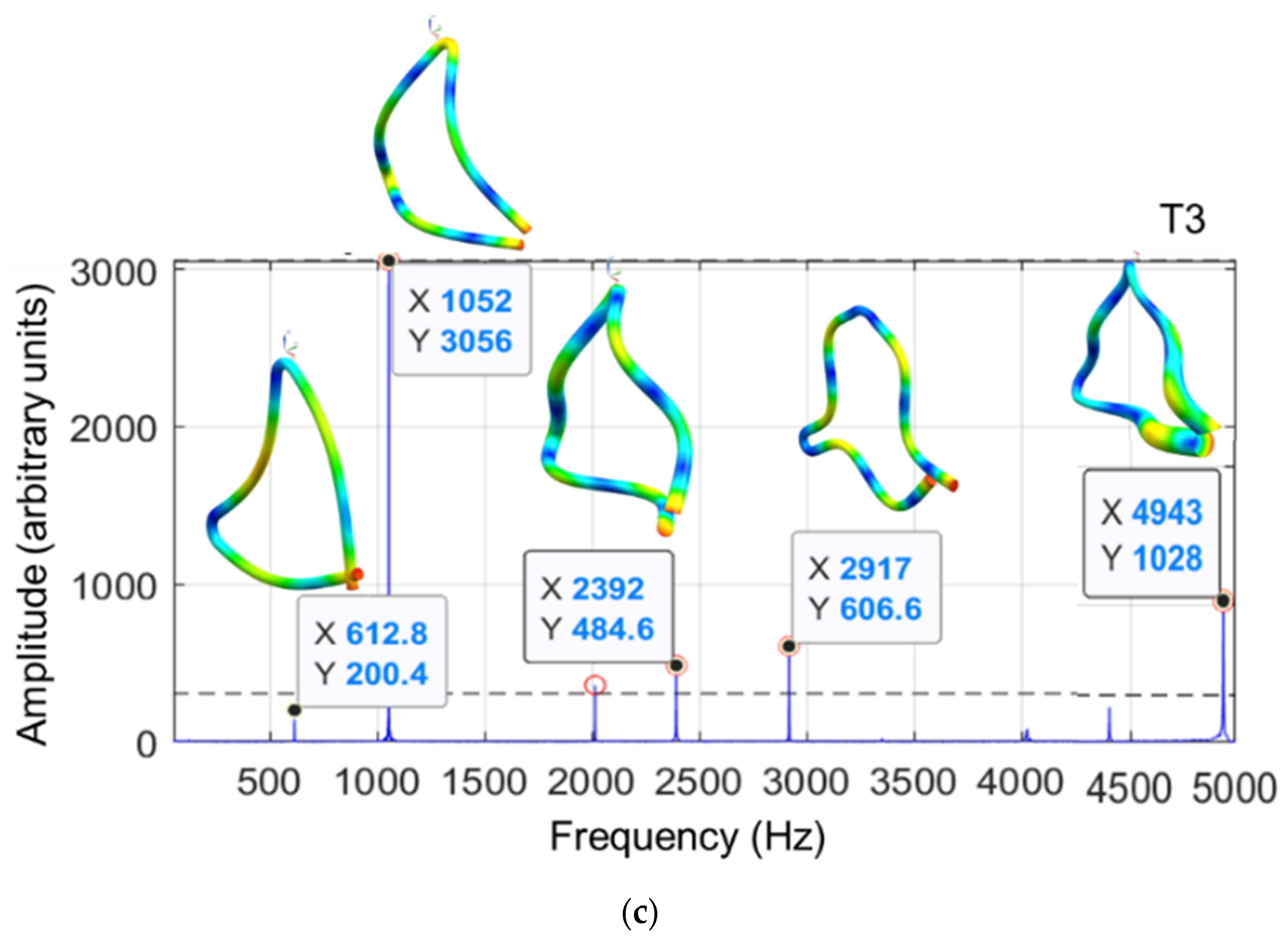
T3	A	96.29	612.70	-	1052.09	1052.09
	B	-	612.83	-	1052.24	1052.24
	C	96.41	612.86	899.70	1045.47	1045.47

.

It was found that the first natural frequency of triangles with similar dimensions (T1 and T2), but different materials, have relatively close values: 168.2 Hz (triangle 2—aluminum) and 159.5 Hz (triangle 1—stainless steel). The T2 aluminum triangle is about twice the mass of the stainless steel triangle, although the length of the sides is about 8% longer than that of the stainless steel T1 triangle. Interestingly, the increase in the sides of the aluminum triangle T3, which is 32% larger than the length of the sides of the triangles T1 and T2, led to a decrease in the value of the first natural frequency by about 42% (from 168 Hz—triangle T2 to 96.5 Hz—triangle T3).

It was observed that when the B side is excited (hit), between the open sides A and C, the first proper frequency is missing, regardless of the analyzed structure. This is due to the contour conditions at the ends of the side, respectively, the bending of the bar at an angle of 60 degrees. Instead, the following natural frequencies have approximately identical values for all three hit sides. The frequency value corresponding to mode 2 is about 13% higher for the stainless steel triangle than for the aluminum structure, which is similar in size. Dimensional variation (increasing the sides of the T3 triangle) decreases the frequency of mode 2 by about 30%.

Analyzing the dominant frequency (the one with the highest amplitude in the frequency spectrum denoted f_Amax), it is found that aluminum triangle type T2 has the highest dominant frequency (1876 Hz), compared to the stainless steel triangle (1657 Hz). Increasing the sides of the triangle (T3) in aluminum reduces the dominant frequency by about 43% compared to the triangle with the smaller sides (T2). Research [4] considers that the sound of a triangle is pleasant if it contains a fundamental sound of several frequencies that are significantly louder than the remaining sound. This remaining sound is without a key, and the sound level is significantly lower than the dominant sound. The spectrum of the high-quality triangle contains four tones that are significantly louder than the others, namely, 1539.1 Hz; 4239 Hz; 5658 Hz; 7795 Hz.

Figure 6, Figure 7 and Figure 8 show the spectrograms of the acquired signals for the three triangles struck on the three sides. Thus, the magnitude of the power spectral density related to time and frequencies is shown by color bar. Excitation of different sides of triangles produces different intensities of their natural frequencies.

In the case of triangle 1, the excitation of side B, located between the other two bent sides, presents the richest spectrum compared to the other two sides (Figure 6c). In opposition to the behavior of triangle 1 is the case of triangles 2 and 3, where side B contains the lowest intensities of its own frequencies, some even missing from the frequency spectrum (Figure 7c and Figure 8c). The excitation force plotted against the time is also attached for each spectrogram (Figure 6b,d,f, Figure 7b,d,f and Figure 8b,d,f).

In the modal analysis performed by the finite element method, the modal shapes of the triangles and the values of the eigenmodes resulted. The values obtained with FEA are in accordance with those determined experimentally, the error being below 2.5%, as can be seen from the graphical comparisons in Figure 9.

Since the experimental results do not provide information about the vibration modes of the triangles, the finite element analysis completes these data, especially since the results obtained by the two methods are in good agreement.

Figure 10, Figure 11 and Figure 12 show the main vibration modes of the triangles. Thus, it is observed that in the case of stainless steel triangle T1, the first mode is characterized by vibrations in the plane of the triangle, for 156 Hz (Figure 10a); the next mode is one of torsion, out of the plane of the triangle, for frequency of 162 Hz (Figure 10b). Then, the triangle vibrates along the axis of the bars, obtaining a longitudinal mode at 269 Hz (Figure 10c). For mode 4, torsional vibrations are obtained out of the plane of the triangle, for 805.285 Hz (Figure 10d), then alternating with longitudinal vibrations along the bar at frequency of 978.74 Hz (Figure 10e), and then bending vibration mode around the z-axis is obtained for 1465.83 Hz (Figure 10f). The next modes are mode 7 (1499 Hz), a bending vibration mode (around the Y-axis) (Figure 10g) and mode 8 (1627 Hz)—bending vibration mode around the Z-axis (out of the plane of the triangle) (Figure 10h).

For the aluminum triangle T2, having dimensions close to the stainless steel triangle (T1), the modal shapes are identical. The values of the natural frequencies differ, being higher than in the case of stainless steel (Figure 11). In the case of the T3 triangle, the same modal shapes occur as for the other two triangles, but at lower frequencies, considering the longer length of the sides (Figure 12).

According to [1], nonlinear mode coupling is obtained both due to the interaction of the shear forces and the tension of the kinked bar, and, on the other hand, due to unbalanced moments across the kink. Similar data were reported by [4], but the modal analyses were performed in order to compare a good triangle to a bad one. In Figure 13, the experimental frequency spectrum and correlation with modal shapes are presented for all three triangles. Figure 13 depicts the correspondence of computational modal shapes to the experimental frequencies within response signal spectrum. The analyses in Figure 13 only take into account the FFT magnitude spectrum. It can be seen that the bending and twisting modes are more and more complex with increasing frequency. At high frequencies, above 2000 Hz, the modes start to differ from one triangle to another.

3.2. Modal Transient Response

For modal transient response, structural damping extracted from experimental tests was used in finite elements analysis (FEA). In

Table 4. The values of damping factor obtained experimental.

Type of Triangle	The Amplitude		Damping Factor	Average Value/STDV
	A1	A2	ξ
T1 (stainless steel)	0.5045	0.4743	0.009824	0.0103 0.0005
	0.5810	0.5462	0.009830
	0.3197	0.2989	0.010707
	0.1482	0.1384	0.010889
	0.1384	0.1296	0.010456
T2 (aluminum)	0.9847	0.8704	0.019637	0.0211 0.0012
	0.8704	0.7606	0.021461
	0.7606	0.6601	0.022555
	0.6601	0.5731	0.022494
	0.5731	0.5076	0.019316

, the values of amplitudes and damping factor are presented. Thus, the average value of the damping factor for aluminum is 0.021, and for stainless steel, 0.01.

Thus, Figure 14a shows the transient analysis of the stainless steel triangle T1 for the node with a maximum displacement of 12.74 mm, located at the end of the free side marked A, the force being applied on the same side. For aluminum triangle T2, the maximum displacement value is 20.24 mm, also recorded in the node at the end of the required side (Figure 14b). This value (T2 triangle—20.24 mm) corresponds to initial transient evolution (the very first steps of evaluation), when external excitation acts. This fact can be also observed within magnitude displacement diagrams (right side of Figure 14)—this high amplitude was shown for just 0.011 s at the beginning of transient evolution. On the other hand, it had to be taken into account that this value is the magnitude of displacement, which contains the displacements along the three axes. In addition, this value can be justified both by the first steps of the specifically computational transitory regime of the numerical algorithm, and by the increment value used in the integration procedure. The vibration amplitude for the T2 triangle, made of aluminum, is about 1.6 times higher than that of stainless steel. This is due to the influence of the damping factor and the physical/elastic properties of the material.

4. Conclusions

The study highlights the differences between the time response and the frequency obtained for different types of kinked rods: two musical triangles with the same dimensions but made from different materials, as well as two musical triangles made from the same materials, but with different dimensions. The paper presents only the results that are able to assure an objective point of view regarding the triangle’s response on impact excitation and its characteristics.

The results show that the frequency spectrum and damping depend on the type of material. Thus, the higher density and modulus of elasticity of stainless steel (three times higher than that of aluminum) leads to a dominant frequency 12% lower than in the case of the aluminum triangle, and a maximum amplitude 1.6 times lower than of the aluminum triangle. The damping factor is two times higher for aluminum than for stainless steel. For the same material, increasing the length of the sides of the triangle by 24% leads to a decrease in natural frequencies by 42%. There is an error of less than 2% between the experimental and numerical results, which confirms that the two methods can be used in addition to understanding the dynamic behavior of triangles.

In future studies, the authors aim to investigate the effects of different musical triangle performance techniques, with the help of a percussionist, on their dynamic behavior.

References

- Peters, G. The Drummer, Man: A Treatise on Percussion; Kemper-Peter Publications: Wilmette, IL, USA, 1975. [Google Scholar]
- Antolli, M.; Ovens, C.; Grieg, E. Peer Gynt Suite No. 1, Op. 46, Teacher Resource Booklet, Tasmanian Symphony Orchestra Pty Ltd. 2019. Available online: https://www.tso.com.au/wp-content/uploads/2019/11/Grieg-Peer-Gynt-Resources-Updated-06112019.pdf (accessed on 2 June 2022).
- Canazza, S.; De Poli, G.; Drioli, C.; Rodà, A.; Vidolin, A. Modeling and Control of Expressiveness in Music Performance. Proc. IEEE 2004, 92, 712–729. [Google Scholar] [CrossRef]
- Clynes, M. Microstructural musical linguistics: Composers’ pulses are liked most by the best musicians. Cognition 1995, 55, 269–310. [Google Scholar] [CrossRef]
- Legge, K.A.; Fletcher, N.H. Non-Linear Mode Coupling in Symmetrically Kinked Bars. J. Sound Vib. 1987, 118, 23–34. [Google Scholar] [CrossRef] [Green Version]
- Blades, J. Percussion Instruments and Their History; Faber and Faber: London, UK, 1974. [Google Scholar]
- Bestle, P.; Hanss, M.; Eberhard, P. Experimental and numerical analysis of the musical behavior of triangle instruments. In Proceedings of the 5th European Conference of Computational Mechanics (ECCM V), Barcelona, Spain, 20–25 July 2014; pp. 3104–3114. [Google Scholar]
- Bucur, V. Mechanical characterization of materials for string instruments. In Handbook of Materials for String Musical Instruments; Springer: Berlin/Heidelberg, Germany, 2016; Chapter 3; pp. 93–132. [Google Scholar]
- Gough, C. Chapter 15—Musical Acoustics. In Handbook of Acoustics; Rossing, T.D., Ed.; Springer: Berlin/Heidelberg, Germany, 2006; pp. 533–667. [Google Scholar]
- Brant-Smith, A. On playing the triangle. Musical Times 1930, 71, 21–22. [Google Scholar] [CrossRef]
- Wotton, T.S. On playing the triangle. Musical Times 1930, 71, 154. [Google Scholar] [CrossRef]
- Rossing, T.D. Acoustics of percussion instruments. Phys. Teach. 1976, 14, 546–556. [Google Scholar] [CrossRef]
- Bărbuceanu, V. Dictionary of Musical Instruments (Dicționar de Instrumente Musicale–in Romanian Language); Grafoart, B., Ed.; Matei Banica: Bucuresti, Romania, 2014. [Google Scholar]
- Bestle, P.; Hanss, M.; Eberhard, P. Musical Instruments–Sound synthesis of virtual idiophones. J. Sound Vib. 2017, 395, 187–200. [Google Scholar] [CrossRef]
- Dunlop, J.I. Flexural vibrations of the triangle. Acustica 1984, 55, 250–253. [Google Scholar]
- Bucur, V. Handbook of Materials for Percussion Instruments; Springer International Publishing: Berlin/Heidelberg, Germany, 2022. [Google Scholar]
- Stanciu, M.D.; Trandafir, M.; Dron, G.; Munteanu, M.V.; Bucur, V. Numerical Modal Analysis of Kinked Bars–Triangle Case of Study. In Proceedings of the 9th International Conference on Modern Manufacturing Technologies in Industrial Engineering, online, 23–26 June 2021. [Google Scholar]
- Rossing, T.D.; Fletcher, N.H. Principles of Vibration and Sound; Springer: New York, NY, USA, 2004. [Google Scholar]
- Flynt, W.E. The Construction and Tuning of Vibrating Bars. Mechanical Music Digest. 2009. Available online: https://www.mmdigest.com/Gallery/Tech/XyloBars.html (accessed on 31 May 2022).
- Trandafir, M. Static and Dynamic Analysis of a Kinked Bars with Different Geometric and Structural Parameters—The Triangle Case of Study (in Romanian Language). Master’s Thesis, Transilvania University of Brasov, Brașov, Romania, 2021. [Google Scholar]
- Product Lifecycle Management Software Inc. Basic Dynamic Analysis User’s Guide-SIEMENS PLM 2014 Siemens. Available online: bhttps://docs.plm.automation.siemens.com/data_services/resources/nxnastran/10/help/en_US/tdocExt/pdf/basic_dynamics.pdf (accessed on 28 April 2022).
- Noor, A.K.; Knight, N.F. Nonlinear dynamic analysis of curved beams. Comp. Meths. Appl. Mech. Eng. 1980, 23, 225–251. [Google Scholar] [CrossRef]
- Wan, Z.-Q.; Li, S.-R.; Ma, H.-W. Geometrically nonlinear analysis of functionally graded Timoshenko curved beams with variable curvatures. Adv. Mater. Sci. Eng. 2019, 2019, 6204145. [Google Scholar] [CrossRef] [Green Version]
- Karmvir, T.; Ramakrishna, K. Overview of methods of analysis of beams on elastic foundation. IOSR J. Mech. Civil Eng. 2014, 11, 22–29. [Google Scholar]
- Shahba, A.; Attarnejad, R.; Semnani, S.J. New shape functions for non-uniform curved Timoshenko beam with arbitrarily varying curvature using basic displacement functions. Meccanica 2013, 48, 159–174. [Google Scholar] [CrossRef]