Limited-Angle CT Reconstruction with Generative Adversarial Network Sinogram Inpainting and Unsupervised Artifact Removal

Abstract

High-quality limited-angle computed tomography (CT) reconstruction is in high demand in the medical field. Being unlimited by the pairing of sinogram and the reconstructed image, unsupervised methods have attracted wide attention from researchers. The reconstruction limit of the existing unsupervised reconstruction methods, however, is to use $[0^{°}, {120}^{°}]$ of projection data, and the quality of the reconstruction still has room for improvement. In this paper, we propose a limited-angle CT reconstruction generative adversarial network based on sinogram inpainting and unsupervised artifact removal to further reduce the angle range limit and to improve the image quality. We collected a large number of CT lung and head images and Radon transformed them into missing sinograms. Sinogram inpainting network is developed to complete missing sinograms, based on which the filtered back projection algorithm can output images with most artifacts removed; then, these images are mapped to artifact-free images by using artifact removal network. Finally, we generated reconstruction results sized $512\times 512$ that are comparable to full-scan reconstruction using only $[0^{°}, {90}^{°}]$ of limited sinogram projection data. Compared with the current unsupervised methods, the proposed method can reconstruct images of higher quality.

1. Introduction

Limited-angle computed tomography (CT) reconstruction is now widely used in such situation as C-arm CT scan [1,2], digital breast tomosynthesis [3,4] and dental tomography [5]. The data of limited-angle CT are incomplete and cannot meet the requirements of Nyquist sampling theorem [6]. As a result, the image reconstructed by the filtered back projection (FBP) algorithm has serious artifacts [7,8], which can affect the detection of the diagnosis of diseases.

Many researchers have conducted in-depth studies on this problem. Iterative reconstruction algorithm [9,10,11,12] was the first to be applied in limited-angle CT reconstruction. For example, Sidky et al. proposed the total variation regularization and projection on convex sets algorithm [13] and the adaptive steepest descent and project onto convex set algorithm [14]. CAI et al. [15] introduced an edge detection strategy into total variation regularization and proposed an edge-guided total variation minimum reconstruction algorithm, and further improved the reconstruction quality through optimization by alternating the direction multipliers. Although the regularization methods have shown some initial success, but they still cannot provide satisfactory results in limited-angle CT reconstruction when a large range of scan angles are missing. At the same time, these solutions also suffer from high computational overhead and slow operation speed.

Along with the development of machine learning technology in recent years, many researchers have applied the supervised convolutional neural network method to the field of CT image reconstruction [16,17,18]. Zhang et al. [19] discovered that the similar striped artifacts between the reconstructed images by the FBP algorithm in limited-angle sinogram reconstruction, so they proposed a neural network feature fitting framework based on the image domain to learn the mapping between images with artifact and artifact-free images. Inspired by research on image restoration in machine vision, Jin et al. [20] believed that performing image completion and predicting missing information in the projection domain is also a viable approach. They used a context encoder to complete the limited-angle sinogram, and then combined it with an iterative algorithm for the reconstruction. The result proved that a sinogram completion method based on context encoder can effectively improve the efficiency and quality of iterative reconstruction. Given that the above methods are performed in a single image domain or projection domain, Zhang et al. [21] proposed hybrid-domain convolutional neural network method, which combined projection domain completion and image domain artifact suppression, but in order to limit the generation of misinformation, supervised constraints from pairs of real sinogram-reconstructed image are necessary [22].

When the amount of training data is sufficient and the network is well trained, the supervised deep learning method can obtain good reconstruction results. In limited-angle CT reconstruction, however, it is difficult to obtain a large number of paired data for supervised training. For this reason, Zhao [23] first proposed the Sinogram Inpainting Network (SIN) method to train the network in an unsupervised manner. SIN consists of two parts: The first part is a U-net-based Generative Adversarial Network, which is used to complete the sinograms; The second part is a U-net Generative Adversarial Network of the same structure to learn the mapping from artifact images to artifact-free images. These two parts are connected by differentiable Radon and inverse Radon transform networks. SIN takes a sinogram of size $256\times 256$ as input and generates a reconstructed image of the same size. The experimental results show that, when the limited angle range is $[0^{°}, {120}^{°}]$, the performance is better than that of the latest simultaneous algebraic reconstruction technique with Total Variation Regularization (SART-TV) [24] in both qualitative and quantitative aspects. Zhou et al. [25] proposed another unsupervised tomography reconstruction adversarial network (Tomo-GAN) based on hybrid-domain optimization. It also consists of two parts: the first part is the Cycle-Consistent Generative Adversarial Networks, which is responsible for mapping the simulation domain sinogram to the real domain sinogram. The second part is the multi-scale conditional GAN, which is developed using both the real-domain sinogram and the corresponding initial FBP reconstruction map as network input. It also introduces a Long–Short-Term Memory to extract features from a sequence of projections from different angles to improve the quality of the reconstruction results. With the above methods, Tomo-GAN successfully enlarged the size of the reconstructed image to $512\times 512$ and significantly reduced the reconstruction time. However, the first part of the network of Tomo-GAN learns the mapping from the simulation domain sinogram to the real domain sinogram in the projection domain and does not restore the missing information of the sinogram, so it does not improve the quality of image reconstruction. Similarly, the minimum range of the scan angle supported by the algorithm remains at $[0^{°}, {120}^{°}]$, and the method will break down when the range is smaller than that. To address the limitations of the methods proposed by Zhao and Zhou, we propose in this paper a generative adversarial network (GAN) sinogram inpainting and unsupervised artifact removal network called SIAR-GAN, which further reduces the angle range limit on the basis of ensuring image quality and image size.

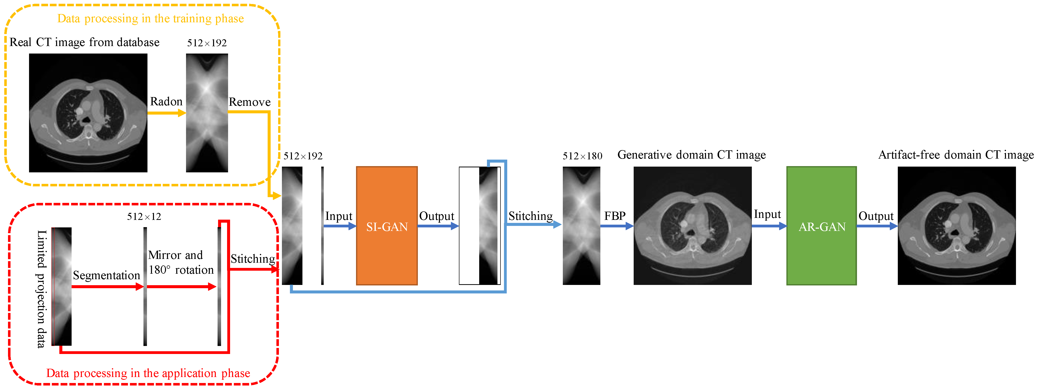
2. Materials and Methods

The SIAR-GAN includes two networks: sinogram inpainting generative adversarial network (SI-GAN) and artifact removal generative adversarial network (AR-GAN). The SI-GAN network is inspired by SIN, and the backbone network also adopts the U-net network structure, and the following improvements are made. Firstly, we designed the size of the input sinogram, so that the area of the network to be completed is not increased as much as possible while increasing the resolution of the sinogram, and the network structure was redesigned to ensure that the designed sinogram can be input into the network normally. The sinogram size design is explained in detail in Section 2.4. Secondly, the SI-GAN network also introduces a cross-layer attention mechanism between the encoders. By calculating the degree of region matching between the patches inside and outside the blank region of missing angles, the feature information is transferred from the outside to the inside of the region, and the performance of the network can be further improved. This part of the content is described in detail in Section 2.1. The AR-GAN network is an improved version of the Cycle-Consistent Generative Adversarial Network (Cycle-GAN), which maps the generative domain CT image to the artifact-free image domain to achieve artifact removal. The training data comes from the unpaired real CT image and the generative domain CT image, and the generative domain CT image is reconstructed from the output of the SI-GAN network with the FBP algorithm. The SI-GAN is introduced to obtain more accurate completed sinogram, based on which FBP algorithm can achieve images with most artifacts removed. AR-GAN can further map images with most artifacts removed to the artifact-free image. The flow chart of the SIAR-GAN algorithm is shown in Figure 1.

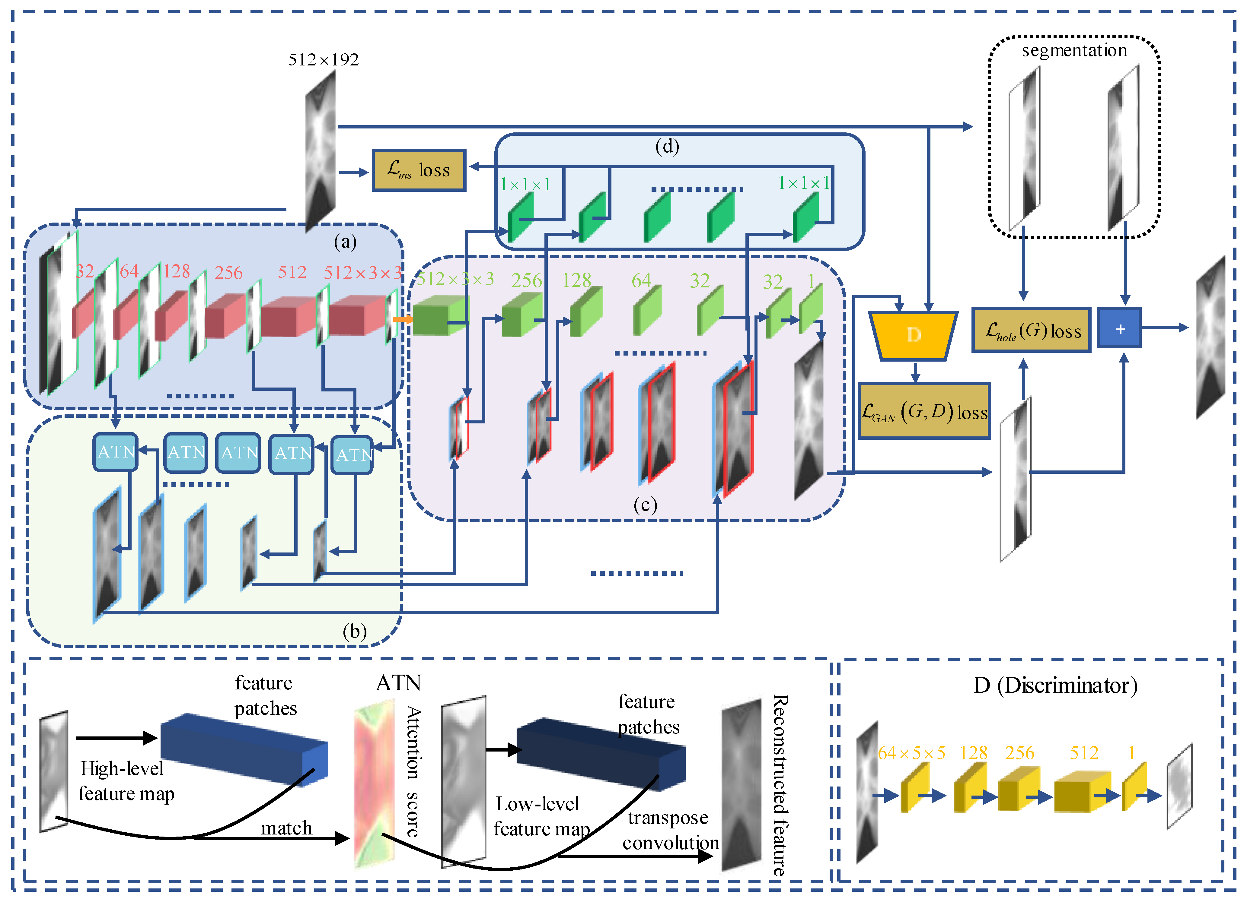
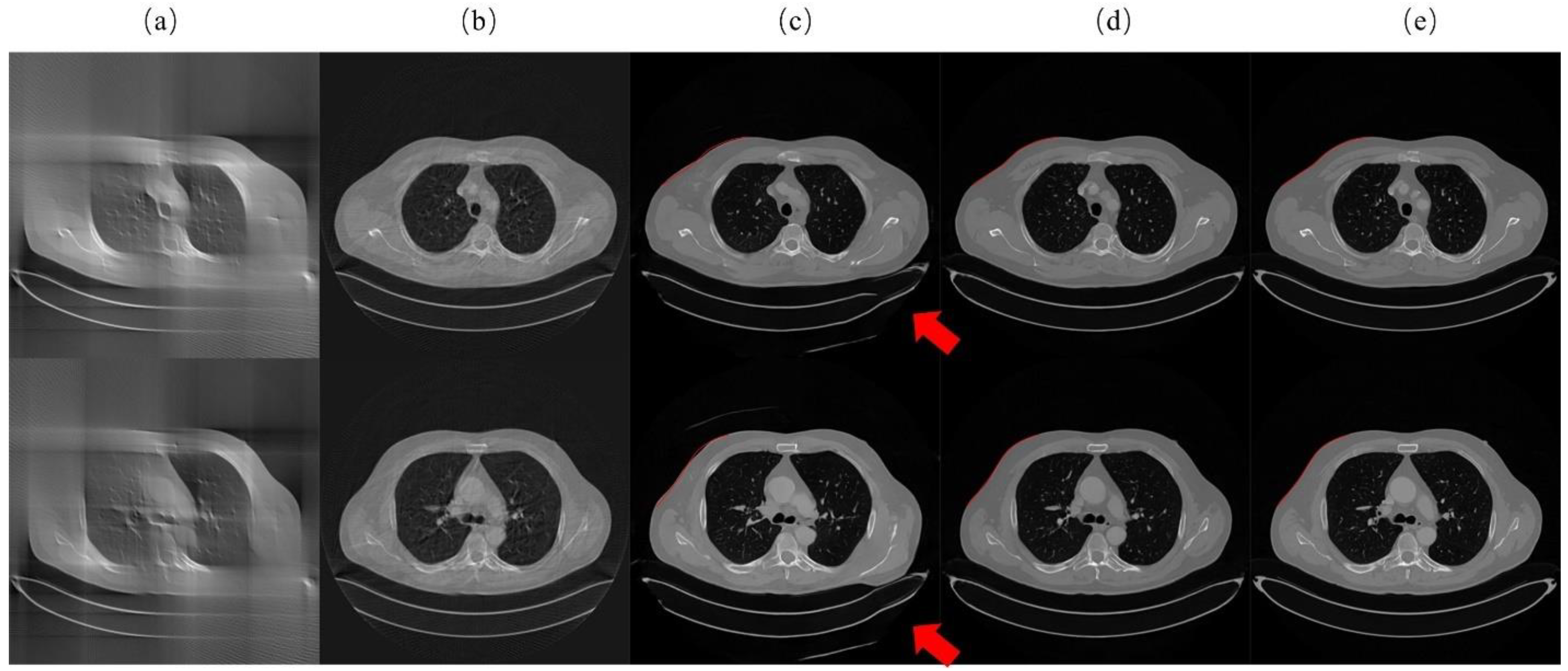
2.1. Sinogram Inpainting Generative Adversarial Network (SI-GAN)

SI-GAN framework is shown in Figure 2. The network encoder module (a) is mainly used to extract the feature information of the limited-angle sinogram, to down-sample the lower-level mask and images layer by layer, and to learn a high-level compact latent feature.

In order to overcome the limitation that encoder module (a) convolves layer by layer and cannot observe image features in the distance effectively, we added the attention module (b). By repeated use of attention network between adjacent layers of encoders and by learning the contents of the high-level semantic feature layer to fill the missing areas of the low-level feature layer, this cross-layer attention filling mechanism can achieve the mapping of high-level semantic features to low-level features, realize a higher resolution, and ensure the content consistency of the missing area. The method of this module drewn on the research of Yu et al. [26] and the implementation details are shown in Figure 2 ATN. By calculating the area matching degree between the ($3\times 3$) patch inside and outside the missing hole area, the external feature information is transferred to the inside of the area. The calculation of the matching degree is gauged by cosine similarity:

$$s_{i,o}^k=\langle \frac{q_{o,n}^k}{\Vert q_{o,n}^k\Vert },\frac{q_{i,m}^k}{\Vert q_{i,m}^k\Vert }\rangle$$

(1)

where $s_{i,o}^k$ represents cosine similarity, $q_{o,n}^k$ denotes the n-th patch extracted outside the hole of the k-th high-level feature map, and $q_{i,m}^k$ represents the m-th patch extracted from the inside of the hole of the k-th high-level feature map. The similarity scores are then processed with SoftMax to obtain the attention score, which is then weighted with the adjacent low-level feature map to fill the hole area:

$$q_{i,m}^{k-1}={\displaystyle \sum _{n=1}^N{\alpha }_{i,o}^k}{q}_{o,n}^{k-1}$$

(2)

where ${\alpha }_{i,o}^k$ represents the attention score calculated through the k-layer high-level feature map, $q_{o,n}^{k-1}$ represents the n-th patch outside the hole of the k-1st low-level feature map, and $q_{i,m}^{k-1}$ represents the m-th patch inside the hole of the low-level feature map of the k-1st layer. The same operation is performed on all patches of adjacent feature layers to obtain the attention-complemented low-level feature map. Finally, the transfer of the attention from the high-level feature map to the low-level feature map is accomplished.

Decoder module (c) simultaneously receives feature images from encoder (a) and attention module (b) in a cross-layer connection. The output feature map of the previous layer of decoder and the output feature map of the corresponding layer of attention module are stacked back and forth, and then input to the next layer of decoder. This is continued recursively to complete filling the missing hole and to form a complete the whole sinogram. The multi-scale decoding module (d) generates images of different scales by convolving with the feature maps of different layers of the decoder and establishes a more rigorous multi-scale loss, so that the model achieves better results.

Unlike many GANs, the discriminator network (D) in this article will output an $59\times 19$ image block instead of a single value. Each pixel value in the image block represents the true probability of the image within the corresponding receptive field in the original image. This regionally aware discriminator can improve the texture and semantic similarity between the generated image and the original image, so that the generated image can have a higher resolution and greater detail.

The loss function plays a key role in the quality of the result of the model and is a basic element in machine learning. In the SI-GAN network, the loss function has three parts: generation adversarial loss, hole loss, and multi-scale L1 loss. The expression of the generation adversarial loss function is:

$${\mathcal{L}}_{GAN}\left(G,D\right)={\mathbb{E}}_{y~P_{data}(y)}\left[\log D\left(y\right)\right]+{\mathbb{E}}_{x~P_{data}(x)}\left[\log \left(1-D\left(G\left(x\right)\right)\right)\right]$$

(3)

where $G$ is the generator network that strives to learn the mapping of $G(x)\to y$ and to generate through $x$ as realistic images as possible that conform to $y$ distribution, $x$ represents the missing projection data, and $y$ denotes the real non-missing projection data. The purpose of discriminator $D$ is to determine as much as possible whether the input image is real or generated by the generator, and $P_{data}$ represents the data distribution.

In order to make the generator generate data that are as real as possible in the missing area of the image, we introduced a hole loss to constrain the optimization results:

$${\mathcal{L}}_{hole}\left(G\right)={\mathbb{E}}_{x~P_{data}(x)}\left[{\Vert \left(y\odot m\right)-\left(G\left(x\right)\odot m\right)\Vert }_1\right]$$

(4)

where m is the mask manually set according to the missing sinogram of the input. The value of the missing portion of the projection data (for example, in $[{91}^{°},{180}^{°}]$) is set as 1, and the value of the rest of the projection data (for example, in $[0^{°},{90}^{°}]$ and $[{181}^{°},{192}^{°}]$) is set as 0, $\odot$ represents a dot multiplication of matrices, and ${\Vert \Vert }_1$ represents the $L_1$ norm. The multi-scale $L_1$ loss limits the output results of each layer of the decoder, so that the output results of each layer are as similar as possible to the original image of the same scale. The loss constraints of different scales can further improve the model performance:

$${\mathcal{L}}_{ms}={\displaystyle \sum _{p=1}^5{\Vert y^p-f\left({\varphi }^p\right)\Vert }_1}$$

(5)

where ${\varphi }^p$ is the output of the p-th layer of the decoder, and the function $f$ encodes the input image into a grayscale image with the same size and a channel number of 1. $y^p$ represents the original image with the same size as ${\varphi }^p$. Finally, we defined the complete loss function as follows:

$${\mathcal{L}}_{SI}={\lambda }_1{\mathcal{L}}_{GAN}\left(G,D\right)+{\lambda }_2{\mathcal{L}}_{hole}\left(G\right)+{\lambda }_3{\mathcal{L}}_{ms}$$

(6)

In this article, the values of the hyperparameters ${\lambda }_1$, ${\lambda }_2$ and ${\lambda }_3$ were, respectively, 0.05, 6, and 0.5.

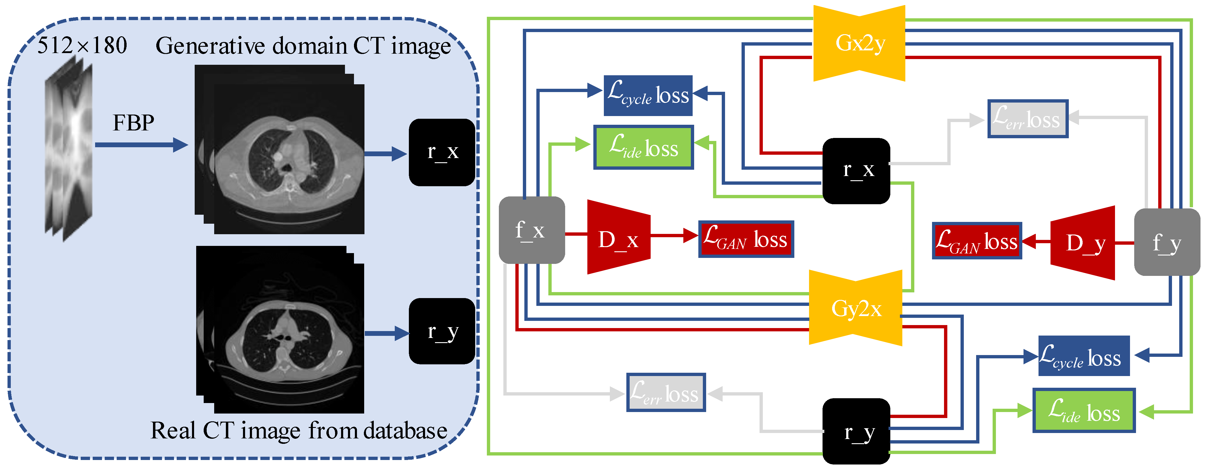
2.2. Artifact Removal Generative Adversarial Network (AR-GAN)

The AR-GAN is constructed on the basis of Cycle-Consistent Generative Adversarial Networks [27], and the generator and discriminator use the same network parameters as the original text. As shown in the AR-GAN framework diagram of Figure 3, the AR-GAN is composed of two generators and two discriminators. The generator $Gx2y$ maps the generation domain CT image $r\_x$ to the $f\_y$ domain through the loss of ${\mathcal{L}}_{cycle}$, ${\mathcal{L}}_{ide}$, ${\mathcal{L}}_{err}$, and the ${\mathcal{L}}_{GAN}$ loss constraint generated by the discriminator $D\_y$. The generator $Gy2x$ is similar.

The loss path of ${\mathcal{L}}_{GAN}$ loss is shown by the red lines in Figure 3. The mathematical expression can be expressed as:

$${\mathcal{L}}_{GAN}\left(Gx2y,D\_y,r\_x,r\_y\right)={\mathbb{E}}_{y~P_{data}(r\_y)}\left[\log D\_y\left(y\right)\right]+{\mathbb{E}}_{x~P_{data}(r\_x)}\left[\log \left(1-D\_y\left(Gx2y\left(x\right)\right)\right)\right]$$

(7)

$${\mathcal{L}}_{GAN}\left(Gy2x,D\_x,r\_x,r\_y\right)={\mathbb{E}}_{x~P_{data}(r\_x)}\left[\log D\_x\left(x\right)\right]+{\mathbb{E}}_{y~P_{data}(r\_y)}\left[\log \left(1-D\_x\left(Gy2x\left(y\right)\right)\right)\right]$$

(8)

The loss of ${\mathcal{L}}_{cycle}$ and ${\mathcal{L}}_{ide}$ can further strengthen the ability of generators $Gx2y$ and $Gy2x$ to generate images of the corresponding domain. ${\mathcal{L}}_{cycle}$ loss path is shown by the blue lines and ${\mathcal{L}}_{ide}$ loss path is shown by the green lines in Figure 3.

$${\mathcal{L}}_{cycle}\left(Gx2y,Gy2x,r\_x,r\_y\right)={\mathbb{E}}_{x~P_{data(r\_x)}}\left[{\Vert Gy2x\left(Gx2y\left(x\right)\right)-x\Vert }_1\right]+{\mathbb{E}}_{y~P_{data(r\_y)}}\left[{\Vert Gx2y\left(Gy2x\left(y\right)\right)-y\Vert }_1\right]$$

(9)

$${\mathcal{L}}_{ide}\left(Gx2y,Gy2x,r\_x,r\_y\right)={\mathbb{E}}_{x~P_{data\left(r\_x\right)}}\left[{\Vert Gy2x\left(x\right)-x\Vert }_1\right]+{\mathbb{E}}_{y~P_{data\left(r\_y\right)}}\left[{\Vert Gx2y\left(y\right)-y\Vert }_1\right]$$

(10)

When $f\_x$ obeys the $P_{data(r\_x)}$ distribution and $f\_y$ obeys the $P_{data(r\_y)}$ distribution, the difference distribution between $r\_x$ and $f\_x$ and the difference distribution between $r\_y$ and $f\_y$ should be very similar. Therefore, we used ${\mathcal{L}}_{\mathrm{err}}$ loss to limit the difference of artifacts. ${\mathcal{L}}_{\mathrm{err}}$ loss path is shown by the gray lines in Figure 3. The mathematical expression is as follows:

$${\mathcal{L}}_{err}\left(Gx2y,Gy2x,r\_x,r\_y\right)={\mathbb{E}}_{x~P_{data(r\_x)}{,}_{y~P_{data(r\_y)}}}\left[{\Vert \left(Gx2y\left(x\right)-y\right)-\left(Gy2x\left(y\right)-x\right)\Vert }_1\right]$$

(11)

We defined the complete loss function as follows, and the parameters ${\alpha }_1$, ${\alpha }_2$, ${\alpha }_3$, and ${\alpha }_4$ were, respectively, 1, 8, 4, and 2:

$${\mathcal{L}}_{AR}={\alpha }_1{\mathcal{L}}_{GAN}+{\alpha }_2{\mathcal{L}}_{cycle}+{\alpha }_3{\mathcal{L}}_{ide}+{\alpha }_4{\mathcal{L}}_{err}$$

(12)

2.3. Comparison Methods and Evaluation Indicators

In order to evaluate the advantages of the method proposed in this paper, it was compared to four other methods, namely, the classical filtered back projection (FBP), SART-TV [24], SIN, and Tomo-GAN. Three indicators were chosen to evaluate the reconstruction performance of the network: root-mean-square error (RMSE), peak signal to noise ratio (PSNR), and structural similarity (SSIM).

2.4. Data and Settings

In order to verify the effectiveness of the SIAR-GAN method proposed in this paper, we collected 13,120 CT lung images of patients from the well-known open source clinical medical image database DeepLesion [28] and 3400 CT head images from the LDCT and Projection data of the Cancer Archives [29]. We expanded the head dataset to 13,600 by data augmentation with direct copy. To facilitate the completion of the information near the ${180}^{°}$ edge of the sinogram, CT image was transformed to sinogram with the size of $512\times 192$ using Radon transform during training phase, and the sampling interval of the projected data was $1^{°}$. Remove part view of the projected data to simulate limited-angle sinograms. This generated missing projection data of $[{90}^{°},{180}^{°}]$, $[{120}^{°},{180}^{°}]$, and $[{150}^{°},{180}^{°}]$, together with sinograms of full projection data, forming a training sample dataset to train SI-GAN. During the application phase, the $[0^{°},{12}^{°}]$ projection data of the sinogram were duplicated before the mirror and ${180}^{°}$ rotation operations were performed, and then the results were used as the projection data corresponding to $[{180}^{°},{192}^{°}]$ of the sinogram. In the lung CT dataset and head CT dataset, 9000 images were used for training and the remaining images were used for testing. We extracted the $[0^{°},{180}^{°}]$ sinogram image from the output of SI-GAN network test set for FBP reconstruction. The reconstruction results and the collected original CT images of patients were used as AR-GAN unpaired datasets. The learning rate of the SI-GAN network was set to 0.0001, the number of epoch was 200, and the batch size was 16. The learning rate of the AR-GAN was 0.0002, the number of epoch was 200, and the batch size was 1. The training time of SI-GAN was 33 h, and the training time of AR-GAN was 95 h. To visualize the convergence of the network, we calculated the PSNR, SSIM, and RMSE Indicator values of the test set after each epoch. Figure 4 shows the averaged PSNR, SSIM, and RMSE Indicator values versus the number of epochs for SI-GAN and AR-GAN. For the sake of fairness to the SIN algorithm and the Tomo-GAN method, we used the same data set and the same epoch as AR-GAN and maintained the training strategy and parameters consistent with original text. The FBP algorithm selects Ram-Lak as the filter function and nearest neighbor interpolation as the interpolation function. Since the literature has not come to a consensus on the data-driven parameters of the setting method, we tuned the SART-TV hyperparameters manually to obtain the best average performance. We finally set 15 iterations for each image, and in each epoch, we took 15 steps of TV with the factors $\alpha =0.06$ and ${\alpha }_s=0.997$, where $\alpha$ denotes the maximum step size for the steepest descent of TV minimization, and ${\alpha }_s$ is the decreasing proportion of $\alpha$ after each calculation.

3. Results

Two examples were used to illustrate the role of SI-GAN and AR-GAN in the proposed network of Section 3.1 and to evaluate the proposed network and baselines qualitatively and quantitatively. Qualitative and quantitative results are included in Section 3.2, Section 3.3 and Section 3.4.

3.1. Comparison with Different Architecture

First, we demonstrated the role of SI-GAN using ${90}^{°}$ limited-angle projection data, as shown in Figure 5. Obvious artifacts exist in FBP reconstruction for ${90}^{°}$ sinogram. The SI-GAN network has effectively completed the missing sinogram, based on which the FBP algorithm can produce images with most of the artifacts removed.

We then displayed the artifact-removed results of AR-GAN in Figure 6. This helps to demonstrate the contribution of AR-GAN. Figure 6a,c shows that AR-GAN can effectively remove the artifacts, but strong inconsistencies are present, as can be seen from the red outline and red arrow in Figure 6c. As expected, the AR-GAN network exhibited excellent performance in eliminating artifacts when the FBP reconstruction of the output of SI-GAN is used as the input. This can be concluded from the comparison of Figure 6d,e.

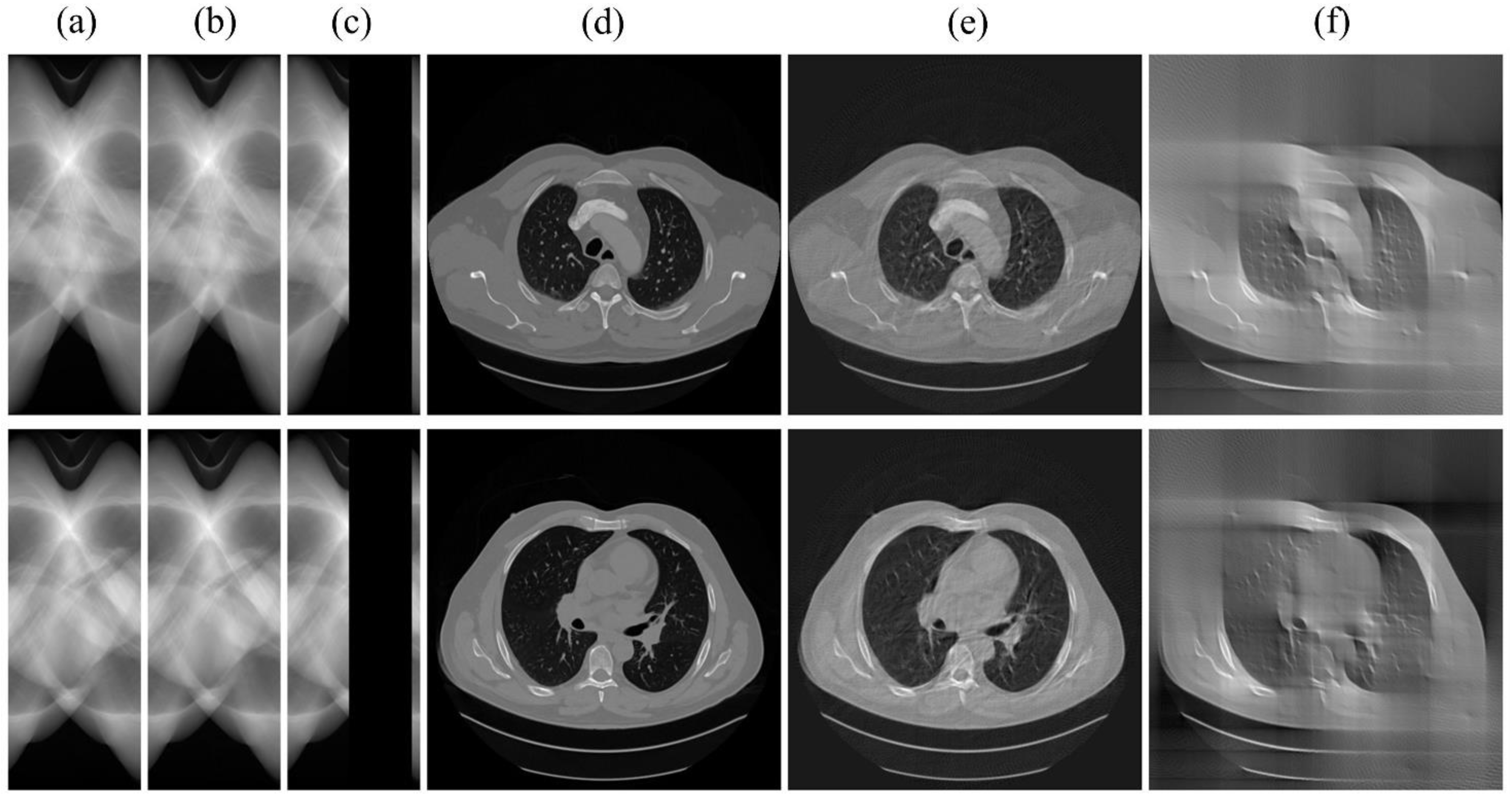
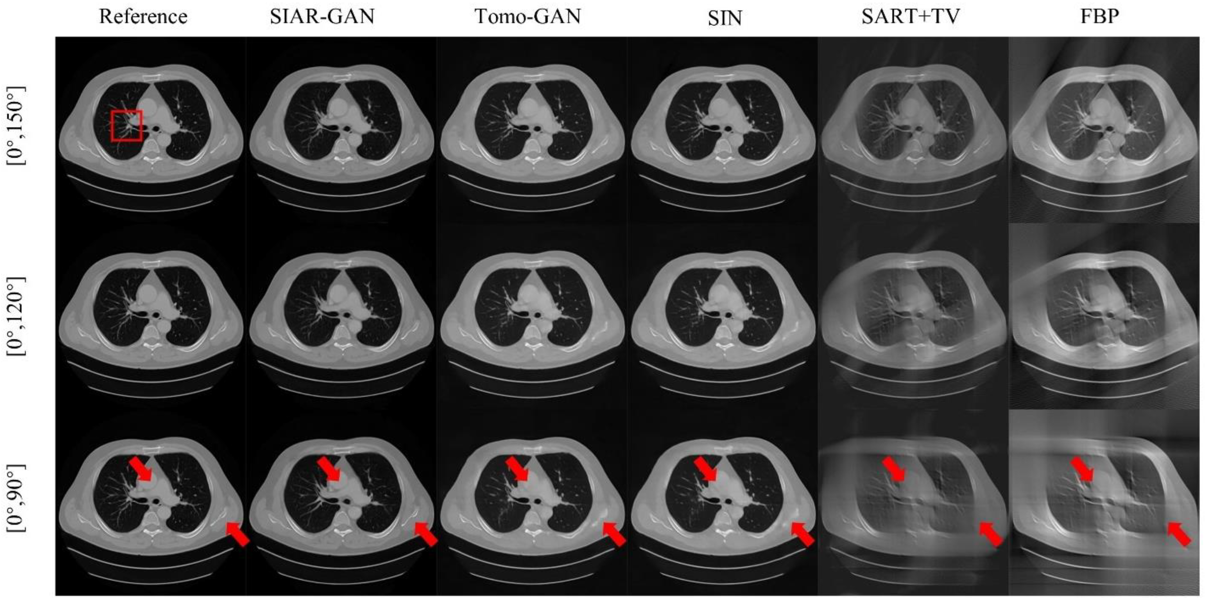
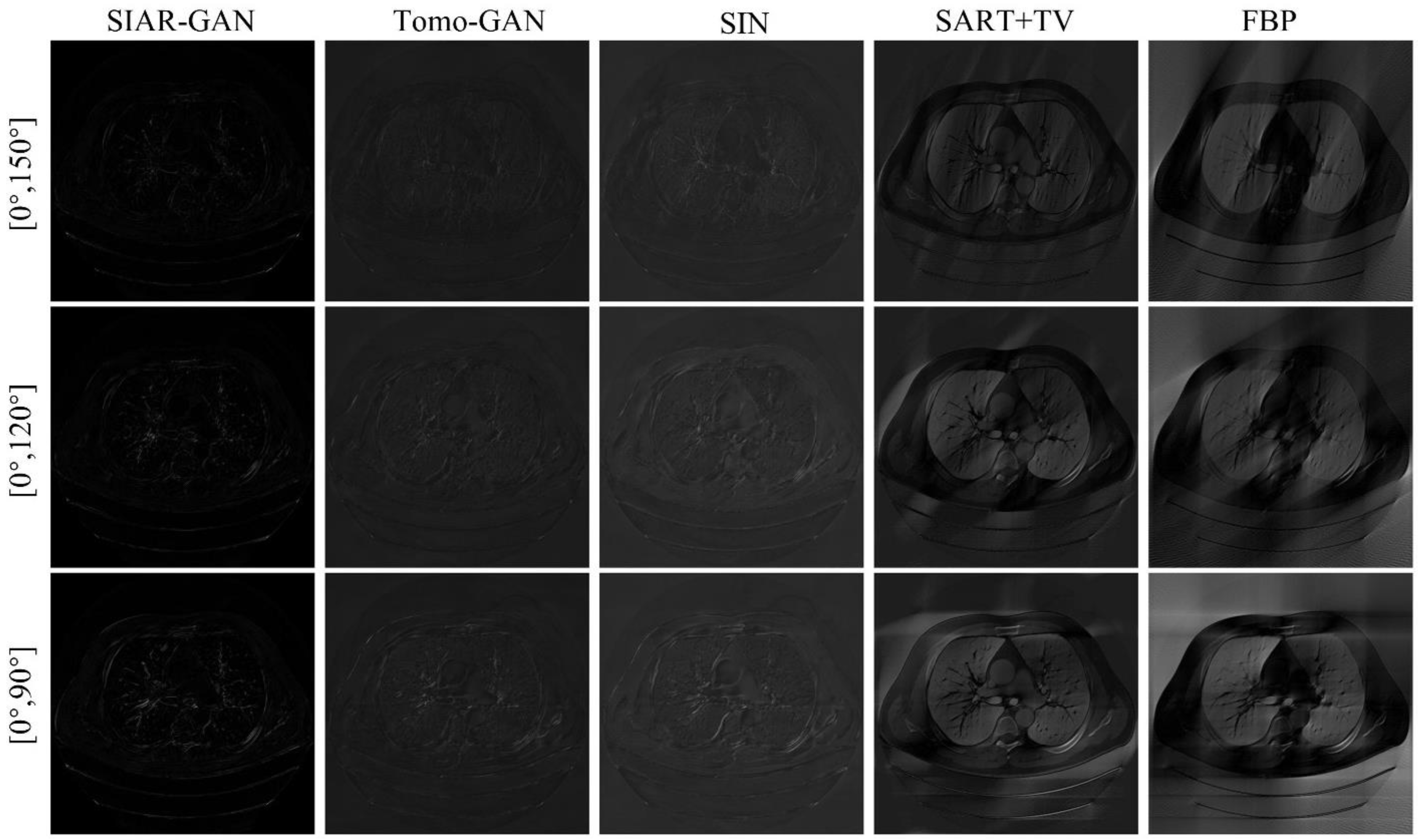
3.2. Qualitative Experimental Results for Lung Data

The full experimental results of lung CT data reconstruction are shown in Figure 7. The reconstruction results of SART-TV and FBP methods become significantly worse as the projection data decreases, especially in the upper left and lower right corners, where the structure and texture have become completely blurred for the $[0^{°}, {90}^{°}]$ projection data. Both Tomo-GAN and SIN are methods based on unsupervised deep learning hybrid-domain artifact removal. Compared with SART-TV and FBP methods, the reconstruction results are significantly improved, but when the projection angle is only $[0^{°}, {90}^{°}]$; they too cannot effectively suppress artifacts and textures, and cannot effectively restore the profile information, as shown in the area corresponding to the red arrows in Figure 7. In contrast, the method proposed in this paper, through joint optimization of projection domain and image domain, played a significant role in suppressing artifacts, and the important structure and texture information of the area corresponding to the red arrows is effectively restored and preserved.

The absolute difference image can further compare the reconstruction results of each method. The results are shown in Figure 8. The smaller difference corresponds to a better reconstruction. The results of these three cases of projection angles all show that the reconstruction quality of the method in this paper works better. Comparing the reconstruction results of $[0^{°}, {150}^{°}]$ and $[0^{°}, {90}^{°}]$, it can be found that the reconstruction quality degrades when less projection data are used.

In order to compare the texture and structural details of the reconstruction results of each method more clearly, we selected the red framed area in Figure 7 to zoom in, as shown in Figure 9. Consistent with the results of the above analysis, the SART-TV and FBP methods exhibited a considerable number of artifacts and only the outline can be distinguished, while the textural details were completely blurred. In the area indicated by the red arrow in Figure 9, part of the structure and contours were not restored correctly, and the textural details were also lost when Tomo-GAN and SIN methods had only a limited angle of $[0^{°}, {90}^{°}]$. In contrast, the SIAR-GAN method not only restored the complete structure, but also retained more textural details. Although there are still some imperfections compared with the reference image, SIAR-GAN produced high quality images that are superior to the other methods according to quantitative evaluation results by the RMSE, PSNR, and SSIM indicators.

3.3. Quantitative Experimental Results for Lung Data

We re-assessed the reconstruction results quantitatively using the entire test dataset and calculated the standard deviation to assess fluctuations in reconstructed image quality. The reconstructed images were obtained using the proposed method and the resultant images were quantitatively analyzed with the three indicators of RMSE, PSNR, and SSIM to obtain an average value; higher PSNR and SSIM values and lower RMSE values correspond to a better reconstruction. The higher quality of sinogram reconstruction from limited angles using our unsupervised deep learning method;

Table 1. Average PSNR results (mean $\pm$ standard deviation).

Angle	FBP	SART-TV	SIN	Tomo-GAN	SIAR-GAN
$[0^{°},{150}^{°}]$	16.3457 ± 1.6106	19.2531 ± 0.5965	26.7125 ± 1.7880	28.9774 ± 1.6971	31.1028 ± 1.5224
$[0^{°},{120}^{°}]$	15.7783 ± 0.9374	18.1774 ± 0.4456	25.3332 ± 1.5566	27.5112 ± 1.6104	30.2231 ± 1.3819
$[0^{°},{90}^{°}]$	13.0208 ± 0.5416	16.7119 ± 0.3335	23.2377 ± 1.1701	25.6884 ± 1.6570	29. 2011 ± 1.3703

,

Table 2. Average SSIM results (mean $\pm$ standard deviation).

Angle	FBP	SART-TV	SIN	Tomo-GAN	SIAR-GAN
$[0^{°},{150}^{°}]$	0.5065 ± 0.0521	0.5321 ± 0.0332	0.8611 ± 0.0356	0.9077 ± 0.0327	0.9390 ± 0.0277
$[0^{°},{120}^{°}]$	0.4503 ± 0.0423	0.4697 ± 0.0271	0.8153 ± 0.0423	0.8803 ± 0.0327	0.9255 ± 0.0304
$[0^{°},{90}^{°}]$	0.3093 ± 0.0316	0.3501 ± 0.0194	0.7013 ± 0.0272	0.8102 ± 0.0524	0.9102 ± 0.0240

and

Table 3. Average RMSE results (mean $\pm$ standard deviation).

Angle	FBP	SART-TV	SIN	Tomo-GAN	SIAR-GAN
$[0^{°},{150}^{°}]$	39.4962 $\pm$ 5.0869	28.2127 $\pm$ 0.9706	13.0721 $\pm$ 2.1081	11.0954 $\pm$ 2.6180	7.3066 $\pm$ 1.4727
$[0^{°},{120}^{°}]$	41.6998 $\pm$ 4.4619	31.7996 $\pm$ 1.6256	15.8862 $\pm$ 2.3972	13.7782 $\pm$ 2.6471	7.9773 $\pm$ 1.4524
$[0^{°},{90}^{°}]$	57.0615 $\pm$ 3.5469	37.0192 $\pm$ 1.4280	19.5390 $\pm$ 1.8999	15.5744 $\pm$ 3.0219	8.8614 $\pm$ 1.6025

show the result of this analysis. The best results are shown in bold.

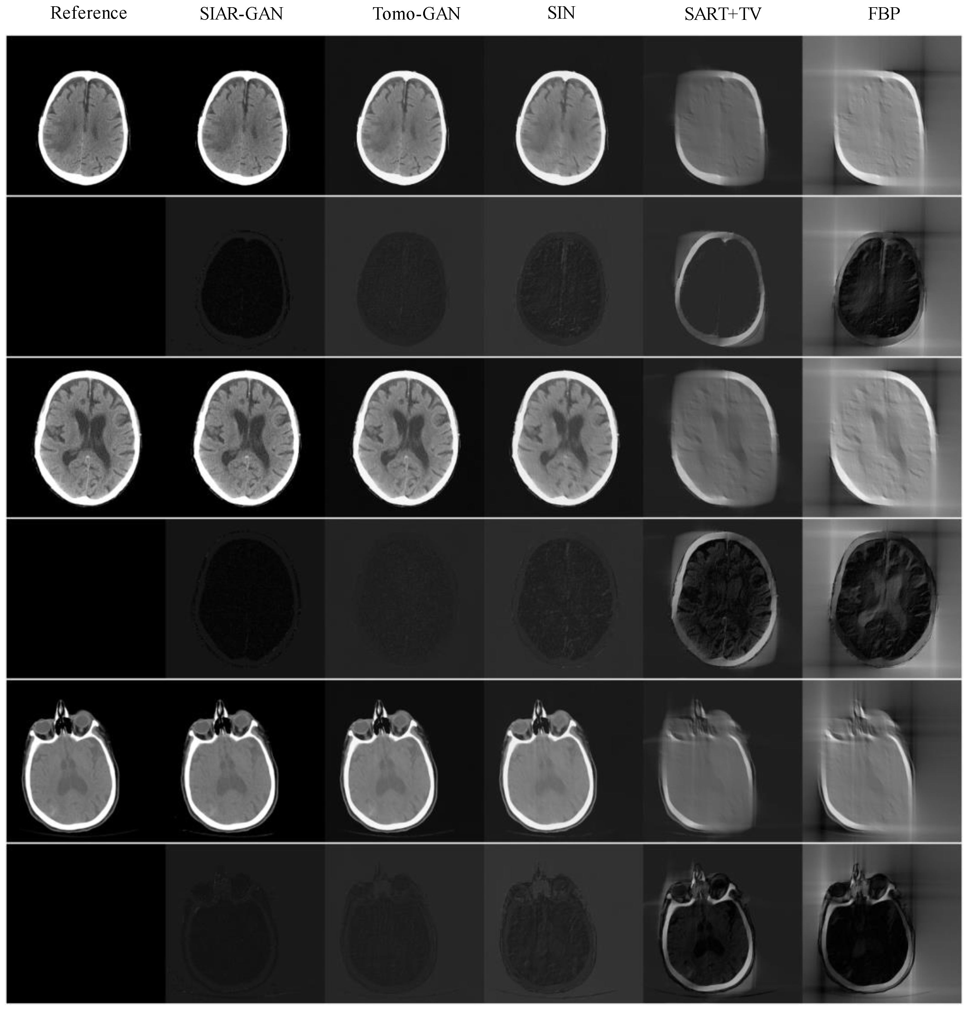
3.4. Qualitative and Quantitative Experimental Results of Head Data

The reconstruction results of head CT data from ${90}^{°}$ projection data are shown in Figure 10. The average PNSR, SSIM, and RMSE results for the reconstruction results of the head CT data from ${90}^{°}$ projection data are shown in

Table 4. Average PNSR, SSIM, and RMSE results for the reconstruction results of the head CT data from the ${90}^{°}$ projection data (mean $\pm$ standard deviation).

Indicator	FBP	SART-TV	SIN	Tomo-GAN	SIAR-GAN
PSNR	10.1629 ± 0.6996	14.7071 ± 0.6204	23.1279 ± 1.6591	25.7152 ± 2.4894	28.7140 ± 1.5467
SSIM	0.2812 ± 0.0339	0.2973 ± 0.0348	0.7249 ± 0.0548	0.7886 ± 0.0597	0.8814 ± 0.0496
RMSE	79.3923 ± 6.2318	47.0200 ± 2.3155	18.1147 ± 3.4723	13.8080 ± 4.5798	9.4966 ± 1.9533

.

Although the reconstruction results of SART-TV are intuitively better than those of FBP, neither of them achieved satisfactory reconstruction results. The main problem of SIN reconstruction results is that there is a certain degree of ambiguity. Both SI-GAN and Tomo-GAN methods obtained reconstruction results similar to the reference, but, from the residual images, the reconstruction results of SI-GAN have less errors. The data in Table 4 demonstrate the above analysis, with the best performing results given in bold.

4. Discussion and Conclusions

It is well known that the amount of training data is a crucial factor that affects the performance of the neural network and the results of limited-angle reconstruction; however, it is often difficult to acquire a large number of sinogram reconstruction data pairs. Moreover, the degree of difficulty in producing reconstruction results of acceptable quality increases with a decreasing amount of angular data in practice. The SIAR-GAN proposed in this paper can be effectively trained without having paired sinogram reconstructed image data. Using an unsupervised method, we generated reconstruction results comparable to full-scan reconstruction with only $[0^{°}, {90}^{°}]$ of limited sinogram projection data on the basis of maintaining a large image size. Compared to other existing unsupervised methods, the proposed method produced images of higher quality according to the evaluation of image quality indicators.

Although the proposed method performed better than other methods in comparison, there are still some limitations. For example, the data distribution of the sinogram dataset has a significant impact on the performance of SI-GAN. Therefore, in practical training and clinical applications, the collected data should come from a certain area of the body that is as small as possible. Moreover, in order to improve the centrality of the data distribution, the sinogram should be guaranteed to have the same scanning starting point. AR-GAN has a huge network structure, which will be limited by computer hardware. To make such a network work well, a GPU with at least 16G memory is required. In addition, the value of the batch size of AR-GAN is 1, which makes training AR-GAN somewhat difficult. For the network to achieve a good performance, it requires a certain amount of experience. An alternative approach, of course, is to increase the batch size, but this would result in an even larger number of GPUs being required. As the experimental results show, the lungs and heads reconstructed by our method have a satisfactory image quality, so our algorithm is expected to work well for a wide scope of clinical applications. However, it is worth noting that the reconstruction results of this method produce some reasonable organizations that do not exist in the reference image; these results are caused by the characteristics of the generative adversarial network. In the future, some structural and profile restrictions should be added to the network to constrain the output of the network to solve such problems. Therefore, manual image quality assessment should be performed prior to clinical deployment to ensure that the SIAR-GAN reconstructed images are of sufficient quality for a given clinical application.

To summarize, our proposed framework model for a limited-angle CT reconstruction network does not rely on the actual sinogram reconstruction image pair. Compared with current unsupervised deep learning hybrid-domain processing methods, our proposed method further reduced the range of the limited angle and generated images of higher quality. In future work, we will impose some structural and profile restrictions on the output of the network to avoid the local feature errors mentioned above. Moreover, we will also conduct network performance tests on projection data that have a lower range than $[0^{°}, {90}^{°}]$ to further explore the limiting effects of the missing data in unsupervised reconstruction.

References

1. Quinto, E.T. Artifacts and Visible Singularities in Limited Data X-ray Tomography. Sens. Imaging 2017, 18, 9.1–9.14. [Google Scholar] [CrossRef] [Green Version]
2. Delaney, A.H.; Bresler, Y. Globally convergent edge-preserving regularized reconstruction: An application to limited-angle tomography. IEEE Trans. Image Process. 1998, 7, 204–221. [Google Scholar] [CrossRef] [PubMed]
3. Nori, J.; Gill, M.K.; Vignoli, C.; Bicchierai, G.; De Benedetto, D.; Di Naro, F.; Vanzi, E.; Boeri, C.; Miele, V. Artefacts in contrast enhanced digital mammography: How can they affect diagnostic image quality and confuse clinical diagnosis? Insights Imaging 2020, 11, 16. [Google Scholar] [CrossRef] [PubMed]
4. Geiser, W.R.; Einstein, S.A.; Yang, W.-T. Artifacts in Digital Breast Tomosynthesis. Am. J. Roentgenol. 2018, 211, 926–932. [Google Scholar] [CrossRef]
5. Mohamed, A.A.H.; Myung Hye, C.; Soo Yeol, L. Half-scan artifact correction using generative adversarial network for dental CT. Comput. Biol. Med. 2021, 132, 104313. [Google Scholar] [CrossRef]
6. Jerri, J.A. The Shannon sampling theorem—Its various extensions and applications: A tutorial review. Proc. IEEE 2005, 65, 1565–1596. [Google Scholar] [CrossRef]
7. Frikel, J.; Quinto, E.T. Characterization and reduction of artifacts in limited angle tomography. Inverse Probl. 2013, 29, 125007. [Google Scholar] [CrossRef] [Green Version]
8. Frikel, J. A New Framework for Sparse Regularization in Limited Angle X-Ray Tomography. In Proceedings of the International Symposium on Biomedical Imaging, Rotterdam, The Netherlands, 14–17 April 2010; pp. 824–827. [Google Scholar] [CrossRef]
9. Lee, S.H.; Yun, S.J.; Jo, H.H.; Song, J.G. Diagnosis of lumbar spinal fractures in emergency department: Low-dose versus standard-dose CT using model-based iterative reconstruction. Clin. Imaging 2018, 50, 216–222. [Google Scholar] [CrossRef]
10. Sun, L.; Zhou, G.; Qin, Z.; Yuan, S.; Lin, Q.; Gui, Z.; Yang, M. A reconstruction method for cone-beam computed laminography based on projection transformation. Meas. Sci. Technol. 2021, 32, 045403. [Google Scholar] [CrossRef]
11. Zhang, W.; Zhang, H.; Wang, L.; Cai, A.; Li, L.; Yan, B. Limited angle CT reconstruction by simultaneous spatial and Radon domain regularization based on TV and data-driven tight frame. Nucl. Instrum. Methods Phys. Res. Sect. A-Accel. Spectrom. Dect. Assoc. Equip. 2018, 880, 107–117. [Google Scholar] [CrossRef]
12. Rao, J.; Ratassepp, M.; Fan, Z. Limited-view ultrasonic guided wave tomography using an adaptive regularization method. J. Appl. Phys. 2016, 120, 113–127. [Google Scholar] [CrossRef]
13. Sidky, E.Y.; Kao, C.M.; Pan, X.C. Accurate image reconstruction from few-views and limited-angle data in divergent-beam CT. J. X-ray Sci. Technol. 2006, 14, 119–139. [Google Scholar] [CrossRef] [Green Version]
14. Sidky, E.Y.; Pan, X. Image reconstruction in circular cone-beam computed tomography by constrained, total-variation minimization. Phys. Med. Biol. 2008, 53, 4777–4807. [Google Scholar] [CrossRef] [PubMed] [Green Version]
15. Cai, A.; Wang, L.; Zhang, H.; Yan, B.; Li, L.; Xi, X.; Li, J. Edge guided image reconstruction in linear scan CT by weighted alternating direction TV minimization. J. X-ray Sci. Technol. 2014, 22, 335–349. [Google Scholar] [CrossRef]
16. Xie, S.; Yang, T. Artifact Removal in Sparse-Angle CT Based on Feature Fusion Residual Network. IEEE Trans. Radiat. Plasma Med. Sci. 2021, 5, 261–271. [Google Scholar] [CrossRef]
17. Higaki, T.; Nakamura, Y.; Zhou, J.; Yu, Z.; Nemoto, T.; Tatsugami, F.; Awai, K. Deep Learning Reconstruction at CT: Phantom Study of the Image Characteristics. Acad. Radiol. 2020, 27, 82–87. [Google Scholar] [CrossRef] [Green Version]
18. Higaki, T.; Nakamura, Y.; Tatsugami, F.; Nakaura, T.; Awai, K. Improvement of image quality at CT and MRI using deep learning. Jpn. J. Radiol. 2019, 37, 73–80. [Google Scholar] [CrossRef]
19. Zhang, H.; Li, L.; Qiao, K.; Wang, L.; Yan, B.; Li, L.; Hu, G. Image Prediction for Limited-angle Tomography via Deep Learning with Convolutional Neural Network. arXiv 2016, arXiv:1607.08707. [Google Scholar]
20. Jin, S.C.; Hsieh, C.J.; Chen, J.C.; Tu, S.H.; Chen, Y.C.; Hsiao, T.C.; Liu, A.; Chou, W.H.; Chu, W.C.; Kuo, C.W. Development of Limited-Angle Iterative Reconstruction Algorithms with Context Encoder-Based Sinogram Completion for Micro-CT Applications. Sensors 2018, 18, 4458. [Google Scholar] [CrossRef] [Green Version]
21. Zhang, Q.; Hu, Z.; Jiang, C.; Zheng, H.; Ge, Y.; Liang, D. Artifact removal using a hybrid-domain convolutional neural network for limited-angle computed tomography imaging. Phys. Med. Biol. 2020, 65, 155010. [Google Scholar] [CrossRef]
22. Li, Z.H.; Cai, A.L.; Wang, L.Y.; Zhang, W.K.; Tang, C.; Li, L.; Liang, N.N.; Yan, B. Promising Generative Adversarial Network Based Sinogram Inpainting Method for Ultra-Limited-Angle Computed Tomography Imaging. Sensors 2019, 19, 3941. [Google Scholar] [CrossRef] [PubMed] [Green Version]
23. Zhao, J.; Chen, Z.; Zhang, L.; Jin, X. Unsupervised Learnable Sinogram Inpainting Network (SIN) for Limited Angle CT reconstruction. arXiv 2018, arXiv:1811.03911. [Google Scholar]
24. Yu, H.; Wang, G. Compressed sensing based interior tomography. Phys. Med. Biol. 2009, 54, 2791–2805. [Google Scholar] [CrossRef] [Green Version]
25. Zhou, B.; Lin, X.Y.; Eck, B. Limited Angle Tomography Reconstruction: Synthetic Reconstruction via Unsupervised Sinogram Adaptation. In Proceedings of the Information Processing in Medical Imaging, IPMI 2019, Hong Kong, China, 2–7 June 2019; pp. 141–152. [Google Scholar] [CrossRef]
26. Yu, J.H.; Lin, Z.; Yang, J.M.; Shen, X.H.; Lu, X.; Huang, T.S. Generative Image Inpainting with Contextual Attention. In Proceedings of the 2018 IEEE/CVF Conference on Computer Vision and Pattern Recognition (CVPR), Salt Lake City, UT, USA, 18–23 June 2018; pp. 5505–5514. [Google Scholar] [CrossRef] [Green Version]
27. Zhu, J.Y.; Park, T.; Isola, P.; Efros, A.A. Unpaired Image-to-Image Translation using Cycle-Consistent Adversarial Networks. In Proceedings of the IEEE International Conference on Computer Vision (ICCV), Venice, Italy, 22–29 October 2017; pp. 2242–2251. [Google Scholar] [CrossRef] [Green Version]
28. Yan, K.; Wang, X.; Lu, L.; Summers, R.M. DeepLesion: Automated mining of large-scale lesion annotations and universal lesion detection with deep learning. J. Med. Imaging 2018, 5, 036501. [Google Scholar] [CrossRef] [PubMed]
29. Moen, T.R.; Chen, B.Y.; Holmes, D.R.; Duan, X.H.; Yu, Z.C.; Yu, L.F.; Leng, S.; Fletcher, J.G.; McCollough, C.H. Low dose CT image and projection dataset. Med. Phys. 2021, 48, 902–911. [Google Scholar] [CrossRef]
Figure 1. The flowchart of SIAR-GAN algorithm.
Applsci 12 06268 g001
Figure 2. A diagram of the SI-GAN network framework. The network consists of 5 modules: (a) encoder module, (b) attention module, (c) decoder module, (d) multi-scale decoding module, and D discriminator module.
Applsci 12 06268 g002
Figure 3. Dataset and AR-GAN framework. The dataset is in the box on the left in the figure and AR-GAN framework is on the right. The two yellow polygons represent the generator, the two red trapezoids represent the discriminator, different colored rectangles represent different loss functions, different colored lines represent different loss paths, and the squares represent the image domain.
Applsci 12 06268 g003
Figure 4. Averaged PSNR, SSIM, and RMSE Indicator values versus the number of epochs for SI-GAN and AR-GAN based on the [ 0 ° , 90 ° ] projection data reconstruction training from lung data.
Applsci 12 06268 g004
Figure 5. SI-GAN inpainting results with 90 ° limited-angle data (one case per row). (a) The ground truth of sinogram; (b) the output of SI-GAN with (c) as input; (c) the original 90 ° limited-angle data; (d) the ground truth of reconstruction image; (e) FBP reconstruction for (b); (f) FBP reconstruction for (c).
Applsci 12 06268 g005
Figure 6. Artifact-removed results of AR-GAN. (a) FBP reconstruction for 90 ° limited-angle data; (b) FBP reconstruction for the output of SI-GAN; (c) Output of AR-GAN with (a) as input; (d) Output of AR-GAN with (b) as input; (e) Ground truth of reconstruction image. The red line is a hand-drawn outer profile of (e). (Best viewed with zoom-in).
Applsci 12 06268 g006
Figure 7. Experimental results on lung CT data. The first, second, and third rows are the results of reconstruction from [ 0 ° ,   150 ° ] , [ 0 ° ,   120 ° ] , and [ 0 ° ,   90 ° ] projection data. The first column is the full-angle reconstructed reference image, and the images in the subsequent columns are SIAR-GAN, Tomo-GAN, SIN, SART-TV and FBP reconstruction results. (Best viewed with zoom-in).
Applsci 12 06268 g007
Figure 8. The absolute difference between the experimental results of each method and the reference results. The pixel range of the images is [0, 255]. (Best viewed with zoom-in).
Applsci 12 06268 g008
Figure 9. A partial enlarged comparison of different methods using partially enlarged image from the red box area in Figure 7. The layout is consistent with Figure 7.
Applsci 12 06268 g009
Figure 10. Reconstruction results of the head CT data from the 90 ° projection data. The first, third, and fifth rows of images are the reconstruction results of each method. The image in the first column in each of these rows is the reference image reconstructed by the standard FBP algorithm using the full scan. The subsequent columns show the images reconstructed by SIAR-GAN (2nd column), Tomo-GAN (3rd column), SIN (4th column), SART-TV (5th column), and FBP (6th column) algorithms. Below each reconstruction result, the residual image obtained by subtracting the corresponding reconstructed image from the reference image is shown. The pixel range of the residual images is [0, 255]. (Best viewed with zoom-in).
Applsci 12 06268 g010