Bolt Loosening Detection of Rocket Connection Structure Based on Variational Modal Decomposition and Support Vector Machines

Abstract

This paper designed a bolt-loosening Support Vector Machines’ conduct detection method with feature vectors comprising eigenvalue decomposition based on Variational Modal Decomposition (VMD) and Singular Value Decomposition (SVD), combined with permutation entropy. Particle Swarm Optimization-Support Vector Machines (PSO-SVMs) are used for small-sample machine learning and can effectively identify and judge the state of bolt preload. The effectiveness of the proposed method is verified in a typical example of a connection structure under random-amplitude impulse loads and Gaussian white noise with different signal-to-noise ratios. The effect of other bolt numbers being arranged is also discussed in the results. This method’s bolt-loosening identification rate is close to 90% under both equal-amplitude and variable-amplitude loads. Following the interference, with a signal-to-noise ratio of 20 dB, the method also has a recognition rate higher than 70% under various working conditions and bolt equipment schemes. The effectiveness of the method was verified by experiments.

1. Introduction

As the pertinent section of the rocket structure (Figure 1 and Figure 2) is mostly connected by bolted flanges, the connection surface cannot maintain the overall continuity of the spacecraft. Therefore, it has specific nonlinear characteristics, which lead to a complex dynamic response under different operating conditions and types of equipment. These nonlinear response characteristics will undoubtedly affect the overall safety and reliability of the structure, so it is necessary to study the mechanical model of bolted flange connection structures to describe such structural responses.

Kim et al. introduced the fine finite-element model of a bolted connection structure into the actual engineering structure for analysis and verified its validity, comparing it with the beam model of the bolted connection structure [3]. Jamia et al. investigated the micro-slip mechanical behavior of the connection surface to develop the framework of an equivalent prediction model and the parameter identification of a bolted connection structure [4]. Beaudoin and Behdinan developed a mechanistic analysis model of the stop flange and illustrated the applicability of bilinear stiffness [5]. Wu and Nassar analyzed the nonlinear behavior of the bolted flange connection structure under tension-bending-torsion conditions through a fine finite-element model [6]. Luan et al. provided a model of the bolted flange connection structure by introducing different stiffnesses to the tension and compression, which explains the mechanism of the transverse and longitudinal coupling vibration of the interstage segment of the spacecraft [7]. Based on this, Lu et al. investigated the bending-torsion-shear coupling of the structure, in which the shear pins are equipped with the spacecraft docking surface, and then analyzed the effect of different parameters on the internal forces of the structure, such as the lateral inclination angle of the shear pin [8]. Tian et al. carried out a simulation analysis and destructive tests, looking at the failure of a bolted flange connection structure of a projectile body under impact loading [9]. Tang et al. developed a simplified model of the bolted joined cylindrical shell structure based on the Sanders shell theory to investigate nonlinear mechanical properties [10,11]. Then, they proposed a micro-slip model to simulate contact friction [12,13]. To simulate the dynamic response of a launch vehicle’s nonlinear bolted flange connection structure, Li et al. suggested a simplified dynamic modeling method based on a static structural analysis [14]. Pan et al. investigated the near-resonant response of a dual-joint structure model driven by harmonic excitation considering the nonlinear stiffness [15].

The present research focuses on the simplified modeling and static/dynamic analysis of the connection structure in the rocket body to study the nonlinear mechanical characteristics of the overall structure. The bolt preload influences the stiffness properties and dynamic characteristics of the connection structure and is a key indicator of structural safety in practical applications. Therefore, research on the detection of bolt preload is very important for the connection structure of the rocket body. However, the research on the characteristics of the bolt preload is not sufficient.

Since it is difficult to practically measure the bolt preload in real time, its failure can-not be detected directly. Therefore, bolt-loosening detection was studied in this work by performing an eigenvalue decomposition based on variational modal decomposition (VMD) and singular value decomposition (SVD). The VMD of the acceleration response data obtained from the finite-element analysis was applied to obtain the intrinsic mode function (IMF). The SVD eigenvalue was decomposed after Hilbert–Huang Transform (HHT), and the feature matrix was comprehensively obtained by combining the permutation entropy. Finally, machine learning based on particle swarm optimization-support vector machines (PSO-SVM) led to the automatic judgment of the bolt preload state on the acceleration data, whose accuracy was verified in a typical example.

2. Automatic Identification of Analysis Methods

To identify the state of bolt preload quickly and accurately, the following process (Figure 3) was constructed in this work. The physical characteristics of the bolted connection structure and the signal characteristics of the acceleration response are comprehensively considered to construct the feature vector, which is imported into the PSO-based SVM to obtain good recognition accuracy. The feature vector consists of two parts: one is the frequency domain feature of the bolted connection structure, which reflects the change in the structural frequency domain feature when the bolt preload force changes through the VMD decomposition and SVD algorithm; the other is the signal feature, which reflects the change in the structural acceleration response signal through the change in the permutation entropy. The method considers both physical and statistical properties, including the mathematical foundation and practicality.

2.1. VMD

In recent years, wavelet transform and empirical mode decomposition have been the most widely used time-frequency analysis methods [16]. However, wavelet transform has some disadvantages: wavelet transforms require an artificial wavelet basis selection and lack self-adaptability. Meanwhile, Heisenberg’s uncertainty principle limits the wavelet transform, reducing the frequency accuracy while increasing the time accuracy. Empirical mode decomposition (EMD) is commonly utilized in signal decomposition, and mechanical defect identification is used after wavelet transform [17]. The EMD technique lacks a strict mathematical foundation for support and suffers from issues such as a low computational efficiency and modal aliasing [18]. Due to its quick calculation ability and excellent signal-to-noise ratio, VMD is a new signal decomposition approach that can successfully suppress modal aliasing.

The VMD algorithm was created by Dragomiretskiy et al. [19] in 2014 as a new signal processing method. This is a non-recursive, adaptive signal decomposition method. To break down each frequency-part of the signal, the optimum solution of the constrained variational problem is obtained during a decomposition by loop iteration to estimate the modal component’s center frequency and bandwidth near the center frequency. The VMD decomposition approach is more durable, has a faster convergence time, is less prone to modal aliasing, and has a stronger mathematical theoretical background than the EMD decomposition method. The VMD algorithm decomposes the signal into a set of bandwidth-limited IMFs with an adaptive quasi-orthogonal variation:

$$u_k\left(t\right)=A_k\left(t\right)\cos \left({\phi }_k\left(t\right)\right)$$

(1)

where A_k(t) is the instantaneous amplitude of u_k(t), u_k(t) is a set of discrete values, and the derivative of φ_k(t) is the instantaneous frequency of u_k(t).

2.2. Permutation Entropy

Permutation entropy (PE) is a useful tool for assessing the illogicality and complexity of time series [20]. PE has the benefit of being computationally simple, and it possesses good anti-interference abilities as well as good nonlinear data resilience. PE has been widely used in signal identification and mechanical fault diagnosis [21,22]. The calculation method is as follows.

Reconstruct the phase space of the time series {x(i), i = 1, 2, …, N}, as follows:

$$\left[\begin{array}{c}X\left(1\right)=\left\{x\left(1\right),x\left(1+\tau \right),\cdots ,x\left(1+\left(m-1\right)\tau \right)\right\}\\ X\left(j\right)=\left\{x\left(j\right),x\left(j+\tau \right),\cdots ,x\left(j+\left(m-1\right)\tau \right)\right\}\\ ⋮\\ X\left(N-\left(m-1\right)\tau \right)=\{x\left(N-\left(m-1\right)\tau \right),\\ x\left(N-\left(m-2\right)\tau \right),\cdots ,x\left(N\right)\}\end{array}\right]$$

(2)

In Equation (2), m is the dimension, and τ is the delay. Arrange the m X(j) vectors in ascending order to obtain J(k) = {j₁, j₂, …, j_m}, where k = 1, 2, …, g, g ≤ m!. There are m different symbols [j₁, j₂, …, j_m] in total m! (m factorial) possible symbol sequences and J(k) is merely one of them. Let the probability of each symbol sequence occurring be P₁, P₂, …, P_g.

Therefore, the permutation entropy with the Shannon entropy form of time series {x(i), i = 1, 2, …, N} is expressed as:

$$H_{E_n}=-{\displaystyle \sum }_{i=1}^n{P}_i\lg P_i$$

(3)

Since PE can estimate the complexity of the signal, PE can be used to estimate the dynamic changes in the signal.

2.3. SVM

Vapnik proposed the Support Vector Machine (SVM) [23], a pattern recognition method with distinct advantages for nonlinear mapping in small sample sets and limiting over-learning, making it particularly well-suited to small-sample data processing. SVM has been widely used to diagnose mechanical defects when there are a few problem samples [24]. The PSO, paired with the SVM approach, is used in this study since the algorithm’s efficiency must be addressed to finish the fault diagnostic procedure. Several training sample points x, and corresponding labels f(x), are provided for the learning process. The training sample can be transferred into a higher-dimensional feature space and separated using a hyperplane, as follows:

$$f\left(x\right)=\omega x+b$$

(4)

where ω is an m-dimensional coefficient vector, and b denotes the constant term. The values of ω and b should be chosen to optimize the hyperplane, the distance between positive and negative samples. As a result, SVM is an optimization problem with the following formula:

$$\underset{\omega ,C,\xi }{\min }\frac{1}{2}{\omega }^T\omega +C{\displaystyle \sum }_{i=1}^N{\xi }_i$$

(5)

where ξ is the relaxation factor and C is the punishment factor. Then the Lagrange coefficient is introduced, translating the problem to a quadratic programming issue with the following equations:

$$\begin{array}{r}\max W(a)={{\displaystyle \sum }}_{i=1}^N{a}_i-{\displaystyle \frac{1}{2}}{\displaystyle \sum }_{i=1}^N{{\displaystyle \sum }}_{j=1}^N{a}_i{a}_{j}f\left(x_i\right)f\left(x_j\right)K\left(x_i,x_j\right)\\ \mathrm{s}.\mathrm{t}.{\displaystyle \sum }_{i=1}^N{a}_{i}f\left(x_i\right)=0,0\le a\le C\end{array}$$

(6)

The main kernel functions in SVM have a linear, polynomial, sigmoid, and radial basis kernel function (RBF), where K(x_i, x_j) is the kernel function that can be used to transform samples into higher-dimensional feature space. The RBF function is the most suitable and widely used function. As a result, RBF is employed as the kernel function in this paper, which is defined as:

$$K\left(x_i,x_j\right)=e^{-g{\left|x_i-x_j\right|}^2},g>0$$

(7)

2.4. Particle Swarm Optimization

SVM theory is founded on the notion of structural risk minimization and has exceptionally distinct benefits in tackling limited samples as well as high-dimensional and nonlinear problems. The particle swarm algorithm (PSO) aims to leverage individual information sharing in group behavior to move the entire group through a continuous adjustment process, resulting in the evolution from disorder to order in the issue-solving space and the optimal solution to the problem [25,26]. The particle swarm approach is used to find the ideal settings for the support vector machine to improve diagnostic accuracy. It has shown excellent results in the field of fault diagnosis and identification. The support vector machine (PSO-SVM) algorithm steps are demonstrated in Figure 4.

When using the support vector machine for classification and judgment, it is necessary to set the penalty factor parameters C and RBF kernel function parameters g in advance. This paper uses the PSO algorithm to find these parameters to obtain a more accurate model.

2.5. Identification Method

Acceleration response data are employed to construct the bolt state identification method in this research. The acceleration response data are decomposed by VMD into each order of IMF (Equation (1)), and subsequently transformed by HHT. The obtained HHT data still contain scattered information, making limited feature recognition calculations problematic for machine learning. Following the HHT transformation (Equation (8)), the multi-value matrix is diagonalized using SVD decomposition to obtain the diagonal matrix (Equation (9)), which aids in SVM learning. Simultaneously, the permutation entropy is computed based on the original acceleration response data. Both types of feature data are combined to form a new feature vector matrix, which is then used to import feature values into SVM learning. The SVM parameters are determined using PSO, and the trained SVM can judge the status of the bolt preload.

$$u_k(t)=H(\omega ,t)=\mathrm{Re}\left\{{\displaystyle \sum }_{j=1}^n{a}_j(t)e^{i\cdot \int {\omega }_j(t)\mathrm{d}t}\right\}$$

(8)

$$H\left(\omega ,t\right)=U\Phi V^T$$

(9)

U_k(t) is the IMF of each order after VMD decomposition. U and V are the decomposition vectors used by the SVD dimensionality reduction decomposition, with U^TU = I, V^TV = I, and Φ = diag [σ₁, …, σ_p/0]. The values of each order of the diagonal part of Φ are used to form the feature vector. To improve the recognition accuracy, the value of PE is also added, and the feature vector is comprehensively formed. Finally, the bolt state identification flow chart is formed, as shown in Figure 3.

3. FEM Case Analysis

The reduced size of the interstage structure of a certain type of rocket body is used to develop a fine finite-element analysis model in this paper (Figure 5). The genuine interstage connection structure is complex, with a typical thin-walled cylindrical shell structure with bolted connections as its major bearing structure. After maintaining the characteristics of the primary load-bearing structure, the structure is adequately simplified, and the influence of the thread is ignored to enable simulation analysis and laboratory tests. Two aviation aluminum alloy shell structures with the same size and material properties were selected, and connected by six bolts at the flange surface, with a length of 340 mm, a wall thickness of 4 mm, a diameter of 295 mm, according to the parameter background of the relevant rocket body’s interstage section. The bolt hole diameter on the flange face is 8.4 mm, and continuous flange thickness is 10 mm. The elastic modulus of the shell structure is 70 GPa, with Poisson’s ratio of 0.3 and a density of 2700 kg/m³. High-strength steel bolts have a 210 GPa elastic modulus, a Poisson’s ratio of 0.3, a density of 7850 kg/m³, a head diameter of 12 mm, and a shaft diameter of 5.7 mm.

ABAQUS software was used to create the finite-element model. The bolt and nut can be merged due to the thread simplicity, and the preload is applied in the form of bolt load. This simplified modeling method, which simplifies the bolt into an I-shaped model in Figure 5, has been applied in previous research [14], and its effectiveness has been proved. However, although the contact relationship is considered in Li’s research [14], the influence of the bolt preload is not considered. This paper further considers the preload in the model. In the ABAQUS Load Manager, the preload is applied as a bolt load, which simulates bolt preload using face pressure. The C3D8R hexahedral mesh, which is separated in the axial direction, is used to assure calculation efficiency and precision. The contact surfaces in the model include the contact between the flange surfaces and the contact between the bolt and the flange surface in Figure 6. All the contact is set to be surface contact with a contact friction coefficient of 0.2 and the friction formula’s penalty function applied. All contact surfaces in the model are set to hard contact in ABAQUS, which means that the augmented Lagrangian method and the penalty approach are used to solve the normal and tangential contact problems according to the research by Dinger [27]. The bottom of the structure is fastened. The following text includes static and dynamic calculations (Load as Figure 7), in which the Static General calculation step in ABAQUS is used for the static calculation, and the Dynamic Implicit calculation step is used for the dynamic calculation. The acceleration response is obtained by applying a continuous impulse load to the top of the structure, performing dynamic computations, and obtaining the acceleration response. The sampling frequency is set to 5000 Hz. The impulse width is 0.2 ms, and the load amplitude is 1000 N. The number of impulses for the same equipment and bolt preload is 20.

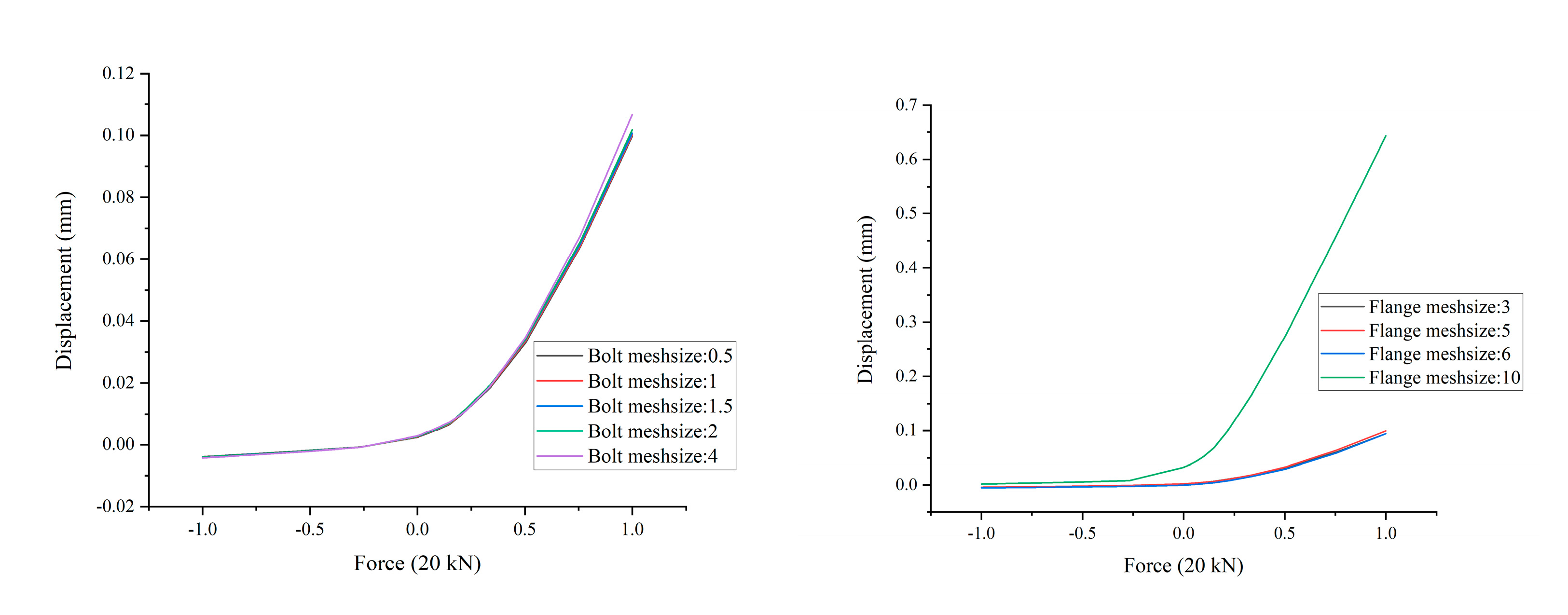
To verify the mesh sensitivity of the finite element model, the meshes of different sizes were applied to the modeling of bolts and flanges. In addition, the calculation was carried out under the same static and dynamic conditions. As shown in Figure 8, the mesh size of the bolt has little effect on the static calculation results, but the mesh size of the flange has a greater effect. When the mesh size of the flange is 10, the calculation result is obviously distorted, and the deviation is very large. When the flange mesh sizes are three, five, and six, the static calculation results are very close, with almost no difference. As shown in Figure 9, in the dynamic calculation results, there is a certain deviation when the bolt mesh size is four, and the results at other sizes are very close. As with the calculation results of the statics, under the dynamic calculation, when the flange mesh size is 10, the maximum acceleration response amplitude deviates greatly, while the results under other mesh sizes have little difference. In summary, considering the computational efficiency and the highest possible accuracy of the results, the mesh size of the bolts used in this paper was 0.5, and the mesh size of the flanges was 5.

The connection structure was assembled with six evenly distributed bolts, and static loads (20 kN top tensile and compressive loads) and continuous impulse loads were applied to the top of the connection to calculate the static and dynamic properties of the structure, respectively. The static load calculation shows that when the bolt is severely loosened, the stiffness at the measuring point significantly decreases under a small load. As the load increases (Figure 10), it tends to be consistent, with no loosening. When the compressive load is applied, whether the bolt is loose or not has little effect on the force-displacement curve of the overall connection structure. The following two equations can be obtained by polynomial fitting of the force-displacement curve data in the tensile load interval:

$$y_{noloosen}=-0.019x^3+0.1x^2+0.015x+0.0025$$

(10)

$$y_{loosen}=-0.042x^3+0.1x^2+0.083x+0.0010$$

(11)

In Equations (10) and (11), y is the displacement and x is the tensile force. The bolts in Equation (10) are not loosened, and the bolts in Equation (11) are severely loosened. It is evident that in the polynomial fitting results, when the tensile force exceeds 18 kN, the slopes of the force-displacement curves of the two are almost the same, and the stiffness at this time is almost the same. However, when the tensile force is small, the stiffness of the two is very different, which indicates that the bolt preload mainly affects the stiffness in the initial stage of loading. Under the top tensile load, the local warpage of the shell is also significantly different due to the difference in the bolt preload (Figure 11). This initial stiffness damage is very detrimental to the structure’s safety and reduces the load-bearing performance of the structure.

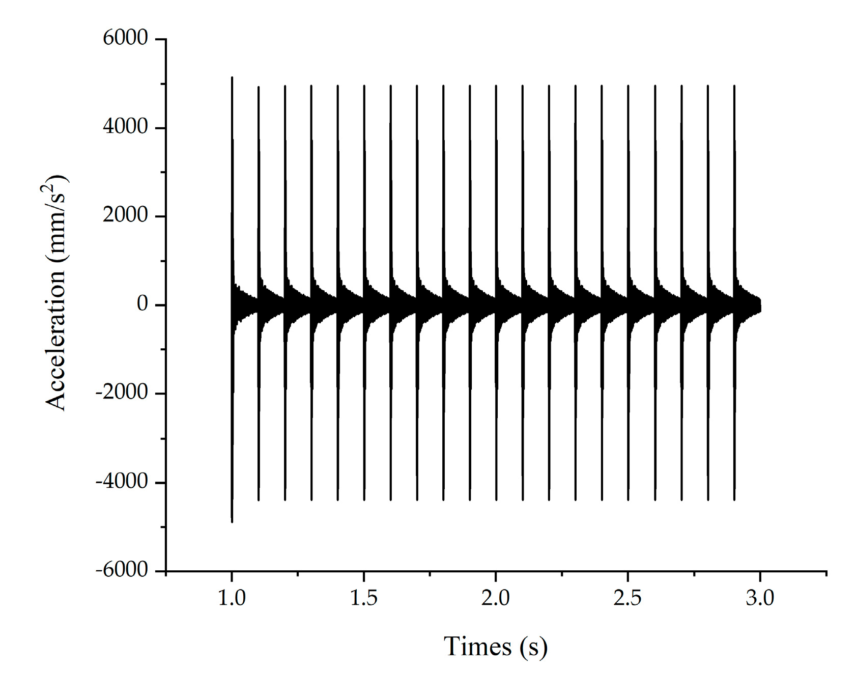
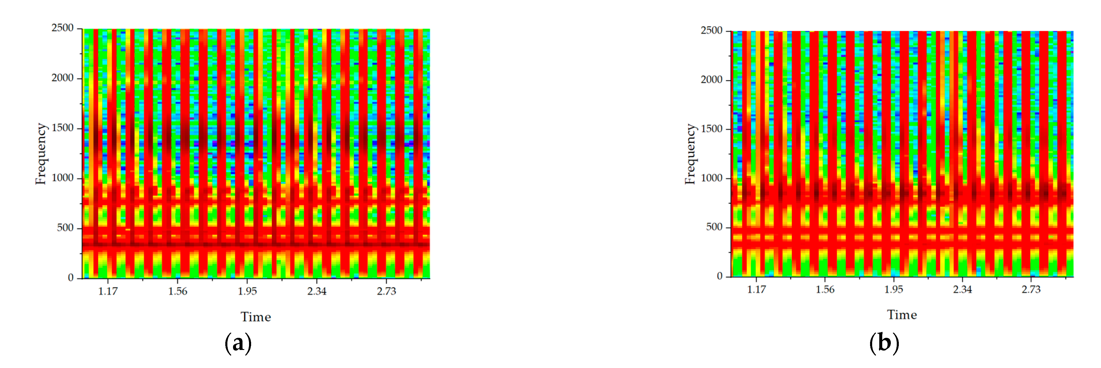
The acceleration response results obtained in the dynamic calculation of the connection structure without loosening are shown in Figure 12. Since reductions in bolt preload in certain locations will cause local stiffness loss, this will inevitably affect the overall continuous impulse response of the connection structure. Therefore, this section adopts the implicit dynamic calculation process to analyze the artificial loosening setting, that is, after the preload is greatly reduced. The response spectrum is obtained after performing a short-time Fourier transform (SFFT) on the acceleration response, as shown in Figure 13, with the color representing the amplitude level. At different times, when a single bolt is loose, the first-order frequency does not significantly change, but it significantly changes with a high frequency. There will be different peaks in the frequency response, which indicate the presence of a loose bolt. This kind of response change in the frequency domain is not intuitive, and although there is an obvious degree of distinction, it is still impossible to directly judge.

Considering that the amplitude of the impulse load often produces a certain amount of change in the actual working conditions, the continuous impulse load with variable amplitude is also calculated (Response results in Figure 14). The amplitude variation in the constant impulse load varies in the form of a random function:

$$F_{amp}=1000\times \left(1-rand\left(0,0.1\right)\right)$$

(12)

The calculation results of implicit dynamics show that the amplitude change has a certain degree of influence on the spectral energy distribution (Figure 15). Therefore, these two situations need to be discussed separately when using SVM for classification prediction. Whether this is the dynamic calculation of constant amplitude or variable amplitude, when the bolt is loosened, the acceleration response spectrum of the structure has some irregular changes. Although this frequency domain change is not intuitive, it is useful for subsequent identification.

When the segment of the acceleration response signal of continuous tapping is extracted for VMD decomposition (Figure 16 and Figure 17), it is evident that when the bolt is severely loosened, the characteristics of the VMD decomposition change to a certain extent, which is beneficial to the designed SVM. From the above spectrogram, it is evident that the first-order frequency of the structure is in the interval between 250 and 500 Hz. Therefore, it is evident that when the VMD is decomposed to the 5th-order IMF, the 1st-order response frequency can be covered. According to this point, the 5th-order IMF data are used in the following paper when using VMD decomposition to design the learning feature matrix.

4. SVM Analysis

In this section, the bolt preload state prediction method proposed above is verified. First, the acceleration data are obtained based on the finite-element model in the previous section, and 500 sampling points are intercepted as one sample. In this research, LIBSVM is employed as a multi-classification SVM algorithm [28,29].

The state of bolt preload is classified under codes (

Table 1. Bolt state label.

Bolt State	Bolt Preload
No loosening	5000 N
Slight loosening	3000 N
Serious loosening	300 N

): classification code 1 is complete bolt pre-tightening (5000 N), classification code 2 is with a slightly loose bolt (3000 N), classification code 3 has a serious loosening of the bolt, almost a failure (300 N), simulating the actual working conditions. During continuous impulse, the acceleration response signal sequence of every 0.1 s is intercepted as a sample. At the same time, to study the universality of the design method in this paper, a variety of equipment and working conditions were analyzed. Training and testing were carried out for the three situations: a 6-bolt arrangement, 8-bolt arrangement, and a 12-bolt arrangement, respectively. The total number of samples for each situation is 60. Machine learning and testing were performed separately for different sample size ratio settings. To be more in line with the project’s actual situation, this paper conducts learning and testing under the original percussion conditions, and then artificially added Gaussian white noise conditions to test the anti-interference performance.

4.1. Continuous Impulse Load of Equal Amplitude

First, the IMF was obtained based only on VMD, and then the feature matrix of SVM learning was acquired through HHT transformation and SVD eigenvalue decomposition. The training set accuracy rate was 100%, and the test set accuracy rate was 83.3% (

Table 2. Prediction accuracy under the condition of equal-amplitude pulse load.

Prediction Accuracy	Feature Vector by VMD	Feature Vector by VMD and PE	Feature Vector by CEEMD	Feature Vector by CEEMD and PE
No loosening (5000 N)	100%	100%	66.67%	83.33%
Slight loosening (3000 N)	83.33%	83.33%	66.67%	66.67%
Serious loosening (300 N)	66.67%	100%	83.33%	100%
Total	83.33%	94.44%	72.22%	83.33%

).

According to the proposed method, the permutation entropy is added to the feature vector to form a comprehensive feature matrix. This new feature matrix is used as the feature value for SVM learning and prediction, and the prediction accuracy is checked. As shown in Table 2, using this method, the prediction accuracy is improved to 94.44%. This shows that the comprehensive feature matrix is a more effective learning feature, verifies the learning accuracy of the method proposed in this paper under small samples, and solves the problem of poor learning accuracy for small samples which has occurred in the past.

VMD is a new modal decomposition technology, so the same effect can be achieved using the old modal decomposition technology as an IMF-acquisition method. The IMF-acquisition algorithm of the method proposed in this paper is replaced with a comparative example made by CEEMD. As an improved algorithm of the original EMD algorithm, CEEMD also has a stronger modal decomposition performance than EMD. As shown in Table 2, the CEEMD-based modal decomposition algorithm is still inferior to our new method (94.4%) in terms of its prediction efficiency (83.3%), even if the permutation entropy is combined as the feature matrix. Therefore, the advanced nature of our newly designed algorithm is proved. Concerning the problem of bolt preload prediction, the VMD algorithm has a better performance than CEEMD.

The data in Table 2 are based on noise-free acceleration response samples, and the method designed in this paper achieved relatively good prediction accuracy. To simulate the needs of actual working conditions, based on the original signal, Gaussian white noise was added to increase the complexity of the signal and test the accuracy of the method. The added white Gaussian noise is described in three labels: one is SNR0, which means no noise; the other is SNR20, which is 20 dB of signal-to-noise ratio; and the third is SNR30, which is 30 dB of signal-to-noise ratio. To quantify a white Gaussian noise signal, the signal-to-noise ratio is defined as [30]:

$$\mathrm{SNR}=10{\log }_{10}\left(\frac{\parallel u\left(t\right)-n\left(t\right){\parallel }^2}{\parallel n\left(t\right){\parallel }^2}\right)$$

(13)

where u(t) is the signal sequence with noise; n(t) is the noise signal sequence.

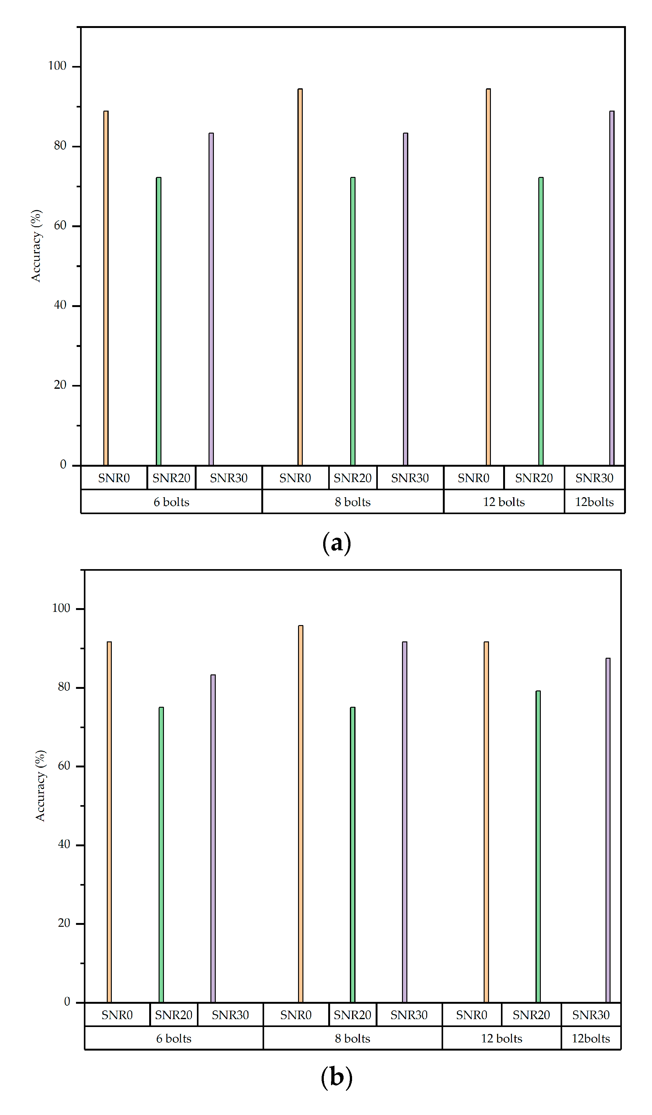
As shown in Figure 18, when 70% and 60% of the total sample points are used as training samples, the method’s accuracy is very close, which shows the effectiveness of the method for learning with smaller samples. It is evident that when the signal-to-noise ratio is 30 dB, the prediction performance decreases slightly. When the signal-to-noise ratio is 20 dB, the prediction performance declines, but the accuracy is still higher than 70%. Under noise interference of this magnitude, the method is still effective, and is effective for different numbers of bolt arrangements, which proves its universality.

4.2. Variable Amplitude Continuous Impulse Load

The previous section predicted the acceleration responses obtained by continuous impulses of equal amplitude using machine learning and SVM, and good prediction results were obtained. However, the load often has a variable amplitude in practical engineering applications. Therefore, a certain number of sample points were obtained based on the finite element model of variable amplitude load calculation and our designed method was used to verify the accuracy of the prediction.

As shown in

Table 3. Prediction accuracy under the conditions of variable-amplitude pulse load.

Prediction Accuracy	Feature Vector by VMD and PE	Feature Vector by CEEMD and PE
No loosening (5000 N)	83.33%	83.33%
Slight loosening (3000 N)	83.33%	50%
Serious loosening (300 N)	100%	100%
Total	88.89%	77.78%

, the prediction accuracy of the SVM, based on the acceleration sample data of the random variable amplitude (10% random amplitude fluctuation, as in Equation (12)), for the bolt preload state is 88.9%, which is lower than the prediction accuracy of the model with equal amplitude shown above, but is still high. This proves the method’s effectiveness, especially for the stochastic load variable amplitude model, which still has a prediction accuracy of nearly 90% under the small-sample learning amount.

As shown in Table 3, when the CEEMD decomposition algorithm is used to construct the feature vectors, the prediction accuracy of the bolt preload state under variable amplitude load drops to 77.78%. In comparison, the method using the VMD algorithm in this paper can still maintain close to 90% accuracy.

We continued to add Gaussian white noise with different signal-to-noise ratios to the acceleration response signal generated by 10% random amplitude fluctuation excitations (Equation (12)), which is consistent with the above signal-to-noise ratio, to simulate the signal fluctuations in actual engineering and increase the interference of the signal.

It is evident from Figure 19 that this method can maintain a high prediction accuracy under the conditions of 10% excitation random amplitude fluctuation. Even under the interference of white Gaussian noise with a signal-to-noise ratio of 20 dB, the accuracy rate remains above 70%.

To further test the performance of this method, we continued to increase the fluctuation range of the excitation amplitude. The range of the random variation in the amplitude was expanded to 30%. This was divided into three levels for comparison: a 10% random fluctuation in amplitude, a 20% random fluctuation, and a 30% random fluctuation. This expands (0,0.1) in Equation (12) to (0,0.2) and (0,0.3). The labels for these three were rand1, rand2, and rand3.

It is evident from Figure 20 that the increase in the random amplitude fluctuation range does not affect the effectiveness of the method proposed in this paper. The change in the accuracy rate caused by the number of samples is that the base of the small sample is small, and the slight modifications to the numerator caused the numerical fluctuation.

This section comprehensively analyzes the effectiveness and universality of the method proposed in this paper through various working conditions, various equipment forms, different random amplitude changes, and artificially added Gaussian white noise, with varying signal-to-noise ratios, and proves the method. It can identify and predict the bolt state in the connection structure of the rocket body based on the acceleration response signal, which has a certain prediction accuracy and plays a guiding role in practical engineering.

5. Experiment Verification

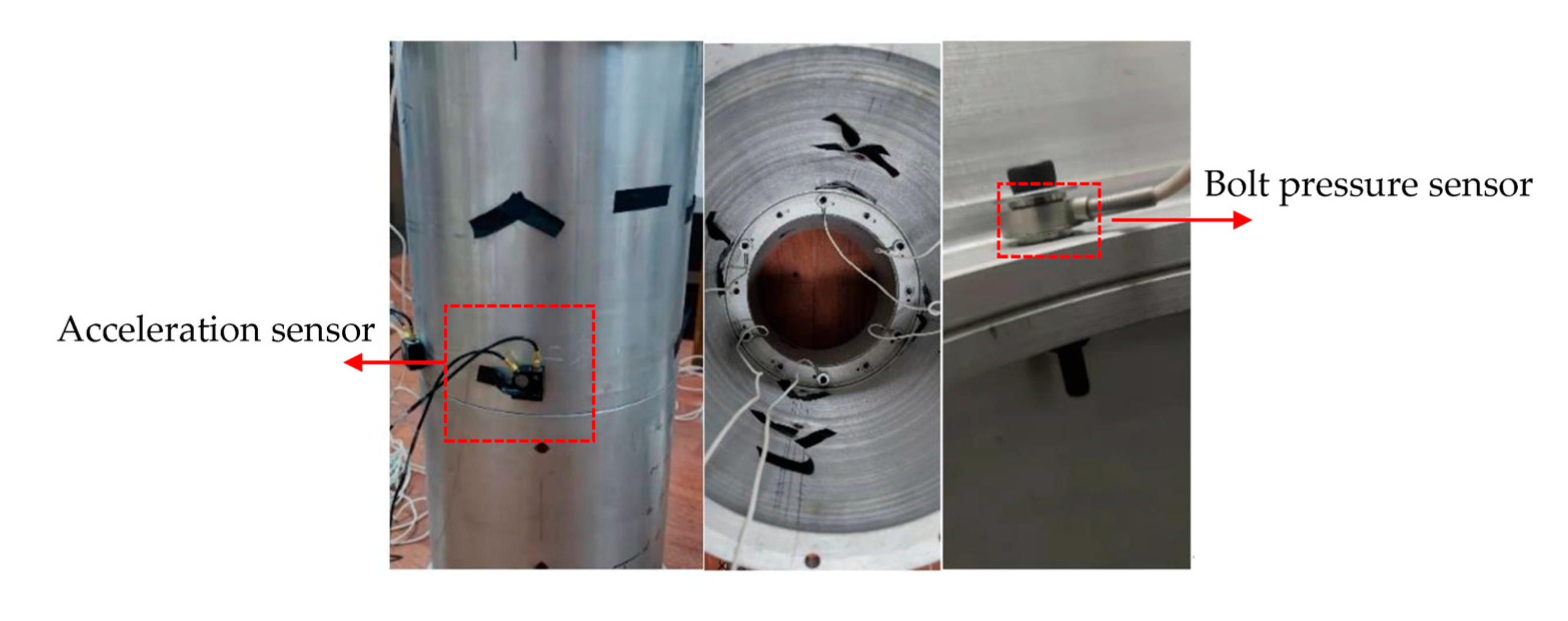
To validate the effectiveness of the proposed loosening detection method, impact experiments were conducted utilizing a bolted flange connection structure (Figure 21), as shown in Section 3. The DH5922D vibration signal acquisition system was used to acquire the acceleration response data. The preload was measured with bolt pressure sensors to ensure the same tension, and the impact load was applied with a force hammer. The bolt grade in the experiment was 12.9. In the experiment, due to the limitations of the experimental conditions, the bolt arrangement was only six bolts, which were evenly arranged. Hammering experiments in loose and unloose conditions were performed to validate the suggested approach, and the acceleration signals of the vibration were obtained. In the experiment, consistent with the finite-element method, 20 strikes were performed under each bolt preload state to simulate the continuous pulse load condition. The magnitude of the force was between 700 and 1000 N. A total of 60 strikes were performed; 70% of the data formed the training group, and 30% of the data formed the verification group.

The experimental data are shown in

Table 4. Prediction accuracy under the experiments.

Prediction Accuracy	Feature Vector by VMD and PE	Feature Vector by CEEMD and PE
No loosening (5000 N)	50%	50%
Slight loosening (3000 N)	83.3%	50%
Serious loosening (300 N)	100%	83.3%
Total	77.78%	61.11%

. The proportion of prediction accuracy is defined as the number of correct predictions over the total number of each case. The method proposed in this paper, based on the VMD decomposition and PE construction of feature vectors to predict the bolt preload state, had an overall accuracy of 77.78% in the experiment. The accuracy in the experiment was lower than that in the finite-element, but the magnitude was limited. There are many reasons for the error in the impact experiment, such as the unavoidable difference between the actual sampling rate and the implicit dynamics calculation, which means that the impact pulse width cannot be completely consistent, and that there was interference in the acceleration signal acquisition. The contact surfaces were all flat in the finite element model, and only the linear friction relationship on the ideal contact surfaces was addressed. However, real experimental settings involve complicated friction interactions as well as intricate local warpage and wear conditions at the connecting contact surfaces. Even under the influence of these error factors, the method proposed in this paper still maintains a certain accuracy, verifying its effectiveness. As shown in Table 4, the experiment also demonstrates that the prediction accuracy when using VMD for feature vector construction, as in this method, is higher than that of CEEMD.

6. Conclusions

In this paper, VMD was used in a modal decomposition to obtain IMF, SVD was used to obtain eigenvalues after HHT transformation, and the permutation entropy of the original signal was calculated. These vectors were combined to obtain a comprehensive feature matrix, and an SVM was established based on PSO. The method combines the physical properties of the structure and the statistical properties of the acceleration signal, taking the mathematical foundation and practicality into account. An example illustrates that this method can accurately identify bolt preload state with a small number of samples. At the same time, the modal decomposition of VMD is also more effective than CEEMD, with better modal decomposition effects. In the past, the modal decomposition algorithm was often used for the fault identification of rotating machines. This paper innovatively applied this to the bolt preload state identification of the rocket body connection structure. Furthermore, the method performs well in terms of various random amplitude excitations and noise interferences. This shows that the modal decomposition algorithm and machine learning method have a wide range of application spaces and use-values in the bolt preload identification of rocket body connection structures. This method has certain engineering value and is helpful in the use and maintenance of the rocket connection structure.