Article

Numerical Simulation of the Kelvin Wake Patterns

1
Navigation College, Dalian Maritime University, No.1 Linghai Road, Dalian 116026, China
2
Shenzhen Pilot Station, Shenzhen 518000, China
3
Marine Engineering College, Dalian Maritime University, No.1 Linghai Road, Dalian 116026, China
*
Author to whom correspondence should be addressed.
Appl. Sci. 2022, 12(12), 6265; https://doi.org/10.3390/app12126265
Submission received: 25 May 2022 / Revised: 16 June 2022 / Accepted: 16 June 2022 / Published: 20 June 2022
(This article belongs to the Section Marine Science and Engineering)

Abstract

:
The ship wave is of great interest for wave drag and coastal erosion. This paper proposes a mechanism of ship wave transformation to explore the effects of ship speed and ship size on the waveform. Firstly, based on the theory of potential flow, the boundary integral equations for the Kelvin ship waves are obtained by deploying the different Kelvin sources or Rankine sources. Then, these integral equations are numerically discretized to a set of nonlinear equations. Finally, the Jacobian−free Newton–Krylov method with a preconditioner is adopted to solve the nonlinear equations. Though imitating plenty of different Kelvin wave patterns, the mechanism of ship wave transformation is proposed to conveniently generate the polymorphic Kelvin wake patterns. The above numerical simulation scheme is verified by comparing simulation results with real ship waves. After that, the wake angle is discussed with the effects of Froude number, source strength and source type by following the mechanism of ship wave transformation. The results show that the wake angle tends to decrease with ship speed but increase with ship size. In addition, for high ship speeds, the effect on the wake angle can be more dramatic.

1. Introduction

When a vessel or a body steadily translates into calm water, free surface waves are generated and these profiles are referred to as “Kelvin ship waves” [1]. The larger the Kelvin wake generated by a ship, the larger the drag force will be on the ship [2]. Meanwhile, the ship waves contain energy, which impacts the coastline and riverbank [3]. Calculating how much the wave drag and knowing how the energy distribution of a ship wave changes with respect to certain properties (e.g., ship speed, ship size and ship shape) can help design the ship hull and inform environmentally friendly shipping policies. Inferring characteristics of wake waveform can help identify ships that have been detected by monitoring instruments [4,5,6].
Initially, Kelvin [7] was fascinated by the V−shaped wake created by a ship advancing through water; one of his most remarkable results concerned the well−known constant wake angle 19.47°, which is known in the community as the Kelvin angle. Lighthill [8] suggested a simplified stationary phase analysis of the dispersion relation, showing that the open dispersion curve is divided by an inflexion into two branches corresponding to transverse waves and divergent waves, respectively. Rabaud [9] noted that for sufficiently fast−moving ships, contrary to commonly held views, the wake angle that is observed behind a steadily moving ship is less than the well−known Kelvin angle, according to simulation results. This finding aroused the interest of many academics. Verberck [10] utilized a steadily moving pressure disturbance to analyze the variation in wake angle for large Froude numbers. Darmon [11] provided an explanation for this phenomenon, namely that the apparent wake angle is naturally provided by lining up the points of maximum wave amplitude along the divergent waves. Furthermore, this is similar for non−axisymmetric simplified ship models and interference effects [12,13,14,15,16], the presence of shear current, submergence depth and finite depth [17,18,19,20], effects of surface tension and the bottom topography [21,22], as well as the effects of viscosity [23]. Pethiyagoda [24] analyzed the wake angles on the low Froude number regime, which arose when the disturbance was traveling sufficiently slowly.
Previously, analytical algorithms were usually utilized to explore ship waves. Havelock [25] firstly presented the linear solution for flow due to a moving point source. Wehausen and Laitone [26] solved the solutions for infinitely deep fluid, as well as fluid of arbitrary finite depth. With the development of numerical methods and computer technology, numerical simulation methods became popular. Meanwhile, the study of ship waves had been extended from two−dimensional linear problems to three−dimensional nonlinear problems. Barbosa [27] used the finite−difference method to solve the three−dimensional free surface hydrodynamical problem. Bettess [28] utilized the finite−element method to explore the flow over a submerged weir. Forbes [29] overcame the difficulty about the singularities and stagnation points of the boundary integral equation, using the boundary integral method in the plane of the physical variables. Wang and Zhu et al. [30] used the high−order boundary element method to solve the steady wave problem of high−speed ships. There are three methods for the discretization of the entire fluid domain: finite−difference method, finite−element method and boundary integral method [31,32,33]. Generally, significant simplifications can be made if the problem is transformed into one involving a boundary integral. By reducing a three−dimensional problem to a two−dimensional problem, the boundary integral method is appealing to solve the three−dimensional nonlinear free surface hydrodynamical problems [34]. Numerical solutions to nonlinear free surface hydrodynamical problems in three dimensions are considerably rare, because of the obvious computational difficulty. Forbes [35] obtained a moderate efficiency by using an inexact Newton’s method. Recently, Pethiyagoda [36] applied the Jacobian−free Newton–Krylov method to solve the fully three−dimensional nonlinear ship wave problem with high efficiency. By combining the boundary integral method with the Jacobian−free Newton–Krylov method, Kelvin wake problems can be investigated efficiently.
Actually, both ship speed and ship size have effects on the wake waveform. However, most previous academics used the different Froude numbers to explore the effect of ship speed on the wake angle, paying little attention to the effect of ship size. Therefore, in order to complement the previous research, this paper proposes a numerical scheme with the mechanism of ship wave transformation to explore the effect of ship size.
In this paper, based on the theory of potential flow, the boundary integral method is used to address the nonlinear free surface hydrodynamical problem. The radiation condition formulation of decay type is used to select a particular solution which does not contain the small spurious waves. Then, the Jacobian−free Newton–Krylov method with a preconditioner is adopted to solve the system of nonlinear equations. After comparing the simulation results with real ship waves, the wake angle is discussed with different Froude numbers, source strengths and disturbances.
This paper aims to indicate the effects of ship speed and ship size on the waveform by imitating different Kelvin wake patterns. The rest of this paper is organized as follows: Section 2 gives the details of the problem formulation; Section 3 describes the numerical method to address the full nonlinear problem; Section 4 compares the simulation results with real ship waves; Section 5 discusses the Kelvin wake angle for the effects of ship speed and ship size; Section 6 presents conclusions and future works.

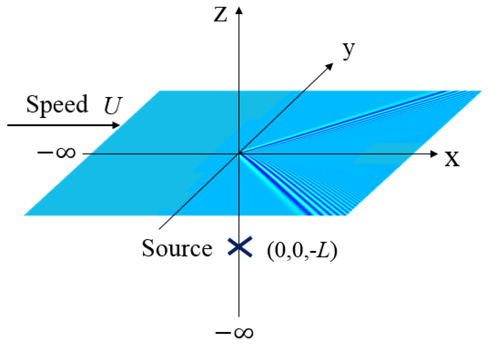
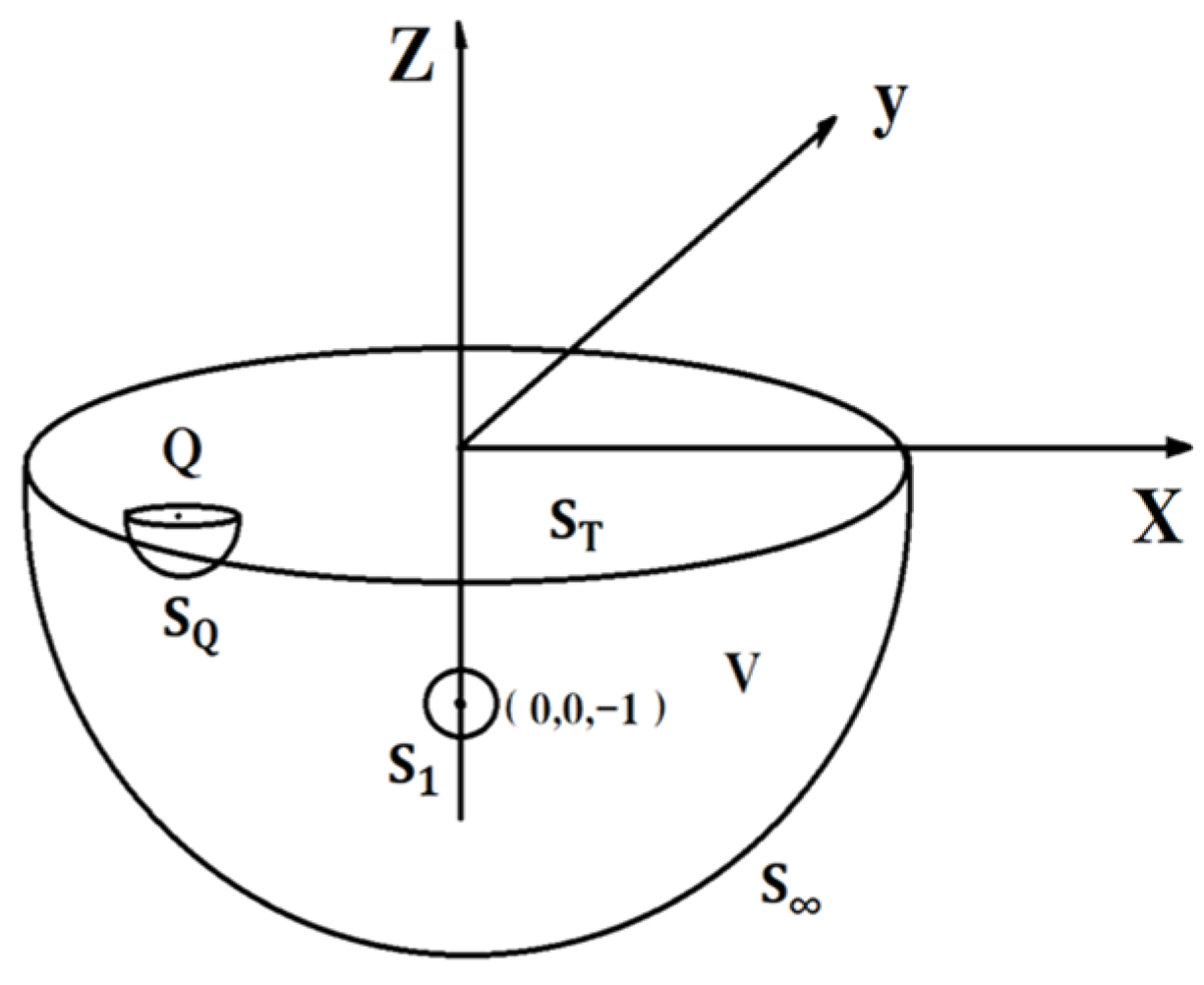
2. Problem Formulation

Based on potential flow theory, this paper considers the irrotational flow of an inviscid, incompressible fluid of infinite depth and ignores the effects of surface tension. The fluid possesses an upper free boundary and is subject to the downward acceleration g of gravity. A Cartesian coordinate is defined such that the x − and y −axes in the plane of the free surface and z axis point vertically with the origin at (0,0,0). The flow is directed along the positive x axis with uniform speed U . Meanwhile, a source singularity whose strength is m or a Rankine source whose strength is κ is introduced at a distance L below the surface, as illustrated in Figure 1. The source strength represents ship size, a higher source strength means a larger ship size. The transient waves will be generated on the free surface, on account of the disturbance caused by a source. This is the steady−state problem, considering the wave pattern does not change over time. The free surface location is described by the equation z =   ζ ( x , y ) , with labelling the velocity potential Φ ( x , y , z ) ; here, the apostrophe means the dimensionless variable. Meanwhile, dimensionless variables can be defined by scaling all lengths with respect to L and all speeds with respect to U .
Assuming the fluid is inviscid and incompressible, Laplace’s equation can be satisfied, as follows:
2   Φ = 2   Φ x 2 + 2   Φ y 2 + 2   Φ z 2 = 0         for   z < ζ ( x , y ) .
By deploying a source point, the velocity potential can be described, as follows:
Φ ~ x ϵ 4 π x 2 + y 2 + ( z + 1 ) 2         as   ( x , y , z ) ( 0 , 0 , 1 ) .
As for the neighbourhood of the Rankine source point, the appropriate limiting behaviour can be described, as follows:
Φ ~ x + μ x 4 π ( x 2 + y 2 + ( z + 1 ) ) 3 2         as   ( x , y , z ) ( 0 , 0 , 1 ) ,  
where ϵ and μ are the Kelvin source strength and Rankine source strength in the form:
ϵ = m U L 2 ,  
μ = κ U L 3 .
Since the kinematic and dynamic boundary conditions must be satisfied on the free surface, the nonlinear conditions are adopted, as follows:
Φ x ζ x + Φ y ζ y =   Φ z                                       on   z = ζ ( x , y ) ,  
  1 2 ( Φ x 2 + Φ y 2 + Φ z 2 ) + ζ F 2 = 1 2             on   z = ζ ( x , y ) ,
where F is the Froude number in the form:
F = U g L .
Finally, the flow will approach the free stream both far upstream and infinitely far below the free surface, the final two conditions are provided, as follows:
( Φ x , Φ y , Φ z ) ( 1 , 0 , 0 ) ,         ζ 0         a s   x ,
(   Φ x ,   Φ y ,   Φ z ) ( 1 , 0 , 0 ) ,                             a s   z .
The problem defined by Equations (1)–(10) can be solved by the boundary−integral method. The field region can be regarded as a half−sphere V whose boundaries are S and S T , except for a small sphere with surface S 1 about the source point (0, 0, −1) and a small hemisphere with surface S Q about typical point Q ( x , y , z ) on the free surface, as shown in Figure 2. Thus, the boundary of the volume V can be written, as follows:
S V = S T + S Q + S 1 + S .  
Given random point P ( ρ , σ , τ ) within volume V , the distance between P and Q is R P Q , which can be described as
R P Q = [ ( ρ x ) 2 + ( σ y ) 2 + ( τ z ) 2 ] 1 2 .  
According to Equation (9), the function Φ x . is harmonic within volume V . As P ( ρ , σ , τ ) . is any point within volume V , it can be proved that the function 1 R P Q is harmonic. Therefore, The Green’s second formula can be satisfied, as follows:
S V [ ( Φ x ) n ( 1 R P Q ) 1 R P Q n ( Φ x ) ] d S = 0 ,
where n denotes the unit normal to the surface.
As shown in Equation (11), the surface integral equation can be divided into four segments. Firstly, when surface S expands to infinity, the result of this partial integration can be described as
lim S S [ (   Φ x ) P n P ( 1 R P Q ) 1 R P Q n P (   Φ x ) P ] d S P = 0 .    
Secondly, the hemispherical surface S Q . shrinks to the surface point Q ( x , y , z ) , which means R P Q tends to zero. Utilizing the mean value theorem of integrals, the result can be described as
lim R P Q 0 S Q [ (   Φ x ) P n P ( 1 R P Q ) 1 R P Q n P (   Φ x ) P ] d S P = 2 π ( ϕ ( Q ) x ) .  
Thirdly, as the spherical surface S 1 collapses to the source point (0, 0, −1), the result of this partial integration can be described as
lim S 1 0 S 1 [ (   Φ x ) P n P ( 1 R P Q ) 1 R P Q n P (   Φ x ) P ] d S P = ϵ [ x 2 + y 2 + ( ζ ( Q ) + 1 ) 2 ] 1 2 .  
Finally, Equation (13) yields
2 π ( ϕ ( Q ) x ) = ϵ [ x 2 + y 2 + ( ζ ( Q ) + 1 ) 2 ] 1 2 + S T [ (   Φ x ) P n P ( 1 R P Q ) 1 R P Q n P (   Φ x ) P ] d S P ,  
where point P now lies on the punctures surface S T .
The integral in Equation (17) can be rendered less singular by subtraction of the following term, which is equal to zero by utilizing Gauss flux theorem,
(   Φ x ) Q S T [ n P ( 1 R P Q ) ] d S P .
Thus, Equation (17) can be re−written, as follows:
2 π ( Φ ( Q ) x ) = ϵ [ x 2 + y 2 + ( ζ ( Q ) + 1 ) 2 ] 1 2 + S T [ (   Φ x ) P (   Φ x ) Q ] n P ( 1 R P Q ) d S P S T [ 1 R P Q n P (   Φ x ) P ] d S P ,
where the symbol n denotes the downward pointing unit normal vector to the free surface and can be written, as follows:
n = ζ x i + ζ y j k ( 1 + ζ x 2 + ζ y 2 ) 1 2 ,
Then the surface integrals become the double integrals by projection onto the x y plane using the following formula:
d s = d x d y | k · n | .  
On the free surface, the velocity potential can be regarded as a function simply of the two independent variables x and y and will be denoted by the symbol ϕ ( x , y ) =   Φ ( x , y , ζ ( x , y ) ) ; the final boundary integral equation can be described, as follows:
2 π ( ϕ ( Q ) x ) = ϵ [ x 2 + y 2 + ( ζ ( Q ) + 1 ) 2 ] 1 2 + 0 [ ϕ ( P ) ϕ ( Q ) ρ + x ] K ( 1 ) ( ρ , σ , x , y ) d σ d ρ + 0 ζ ρ ( P ) K ( 2 ) ( ρ , σ , x , y ) d σ d ρ ,
where the kernel functions K ( 1 ) ( ρ , σ , x , y ) and K ( 2 ) ( ρ , σ , x , y ) are described, as follows:
K ( 1 ) ( ρ , σ , x , y ) = ζ ( P ) ζ ( Q ) ( ρ x ) ζ ρ ( P ) ( σ + y ) ζ σ ( P ) [ ( ρ x ) 2 + ( σ + y ) 2 + ( ζ ( P ) ζ ( Q ) ) 2 ] 3 2 + ζ ( P ) ζ ( Q ) ( ρ x ) ζ ρ ( P ) ( σ y ) ζ σ ( P ) [ ( ρ x ) 2 + ( σ y ) 2 + ( ζ ( P ) ζ ( Q ) ) 2 ] 3 2 ,
K ( 2 ) ( ρ , σ , x , y ) = 1 [ ( ρ x ) 2 + ( σ + y ) 2 + ( ζ ( P ) ζ ( Q ) ) 2 ] 1 2 + 1 [ ( ρ x ) 2 + ( σ y ) 2 + ( ζ ( P ) ζ ( Q ) ) 2 ] 1 2 .  
Moreover, the free surface conditions can be simplified by the symbol ϕ ( x , y ) . Then, the kinematic and dynamic boundary conditions of the free surface are combined to be
( 1 + ζ x 2 ) ϕ y 2 + ( 1 + ζ y 2 ) ϕ x 2 2 ζ x ζ y ϕ x ϕ y 2 ( 1 + ζ x 2 + ζ y 2 ) + ζ F 2 = 1 2 .  
In conclusion, the boundary integral method is used to obtain the boundary integral Equation (22), which identically satisfies Laplace’s equation, the limiting condition (2) and the far−field conditions (9) and (10). Meanwhile, the boundary integral equation should satisfy the combined free surface condition (23); thus, we are left to solve Equations (22) and (23), and the functions ζ and ϕ constitute the solution of the present problem.

3. Numerical Methods

3.1. Numerical Discretization

To solve the nonlinear problem numerically, the x coordinates and y −coordinates of nodes in the N × M mesh are x 1 ,   x 2 ,   ,   x N and y 1 ,   y 2 ,   ,   y N with intervals Δ x and Δ y in the x and y directions, respectively. The free surface elevation ζ ( x , y ) and the velocity potential ϕ ( x , y ) are represented by discrete point values ζ k , l and ϕ k , l at the nodes ( x k , y l ) , k = 1 ,   ,   N ,   l = 1 ,   ,   M . Further, this paper chooses the x derivatives of the functions ϕ and ζ as the basis for the solutions, together with the values of ϕ and ζ at the upstream boundary of the truncated domain, resulting in the vector of 2 ( N + 1 ) M unknowns u to be
u = [ ϕ 1 , 1 , ( ϕ x ) 1 , 1 ,   ,   ( ϕ x ) N , 1 ,   ,   ϕ 1 , M ,   ( ϕ x ) 1 , M ,   ,   ( ϕ x ) N , M , ζ ,   ( ζ x ) 1 , 1 ,   ,   ( ζ x ) N , 1 ,   ,   ζ 1 , M ,   ( ζ x ) 1 , M ,   ,   ( ζ x ) N , M ] T .
Figure 3 shows the distribution of u at an N × M mesh, where ϕ is located at the left side of the mesh, represented by these black dots; ϕ x is located at each node, represented by these congruent triangles. The distribution of ζ and ζ x . works in the same way.
To solve this problem, the vector u is firstly initialized. Then, the remaining ζ can be obtained by trapezoidal−rule integration using ζ x :
ζ k + 1 , l = ζ k , l + 1 2 Δ x ( ( ζ x ) k , l + ( ζ x ) k + 1 , l ) ,   l = 1 ,   ,   M , k = 1 ,   ,   N 1 .
Once ζ is determined, it is facile to compute ζ y by fitting a cubic spline through the nodes ζ k , 1 ,   ,   ζ k , M for k = 1 ,   ,   N . With the same method, ϕ and ϕ y at each node can be calculated by using ϕ x
ϕ k + 1 , l = ϕ k , l + 1 2 Δ x ( ( ϕ x ) k , l + ( ϕ x ) k + 1 , l ) , l = 1 ,   ,   M , k = 1 ,   ,   N 1 .
The boundary integral equation should be reformulated again, because there is a singularity in the second integral of Equation (14). It can be rewritten, as follows:
y 1 y M x 0 x N [ ζ ρ ( P ) K ( 2 ) ( ρ , σ , x , y ) ζ x ( Q )   S ( 2 ) ( ρ , σ , x , y ) ] d σ d ρ + ζ x ( Q ) I ( Q ) ,
and
I ( Q ) = y 1 y M x 0 x N   S ( 2 ) ( ρ , σ , x , y ) d σ d ρ .
where the kernel function S ( 2 ) ( ρ , σ , x , y ) can be described, as follows:
S ( 2 ) ( ρ , σ , x , y ) = 1 A ( ρ x ) 2 + B ( ρ x ) ( σ y ) + C ( σ y ) 2 + 1 A ( ρ x ) 2 B ( ρ x ) ( σ + y ) + C ( σ + y ) 2 ,
A = 1 + ζ x 2 ( Q ) ,
  B = 2 ζ x 2 ( Q ) ζ y 2 ( Q ) ,
C = 1 + ζ y 2 ( Q ) .
Now, the integral I ( Q ) contains the singularity and is computed exactly in terms of logarithms:
  d s d t [ A s 2 + B s t + C t 2 ] = t A 1 2 ln ( 2 A s + B t + 2 [ A ( A s 2 + B s t + C t 2 ) ] 1 2 ) + S C 1 2 ln ( 2 C t + B s + 2 [ C ( A s 2 + B s t + C t 2 ) ] 1 2 ) + h 1 ( s ) + h 1 ( t ) .  
Equation (9) is called the radiation condition; it can select the particular solution that does not contain the small spurious waves. By using the different radiation condition formulations, the results of different accuracies can be obtained [37]. Generally, plausible candidates for the radiation condition include requiring that far upstream:
  • The free surface elevation is zero;
  • The vertical component of velocity is zero;
  • The free surface elevation decays exponentially;
  • The vertical component of velocity decays exponentially.
By investigating these radiation condition formulations, the radiation conditions of class 4 are more successful in selecting the particular solution, which does not contain the small spurious waves. The radiation condition can be enforced near the upstream end of the computational domain. However, in the present problem, only horizontal components need to be solved. The vertical component of velocity is the function that consists of the horizontal components of velocity and elevation, as shown in Equation (6). Thus, the radiation condition formulations of the vertical component of velocity decaying exponentially should be reasonably altered. This paper enforces an equation in the form x f x + n f = 0 along the boundary x = x 1 for the horizontal components of velocity and free surface elevation decaying exponentially. There are 4 M equations by applying the radiation condition for l = 1 ,   ,   M , as follows:
x 1 ( ( ϕ x ) 1 , l 1 ) + n ( ϕ 1 , l x 1 ) = 0 ,
x 1 ( ϕ x x ) 1 , l + n ( ( ϕ x ) 1 , l 1 ) = 0 ,  
x 1 ( ζ x ) 1 , l + n ζ 1 , l = 0 ,  
x 1 ( ζ x x ) 1 , l + n ( ζ x ) 1 , l = 0 ,  
where n is the decay coefficient.
In conclusion, there are totally 2 ( N + 1 ) M equations to be solved for the 2 ( N + 1 ) M unknowns in the nonlinear ship wave problem. The boundary integral equation has been discretized to the ( N 1 ) M nonlinear equations, and additional ( N 1 ) M nonlinear equations are given by evaluating the free surface condition at the half mesh points, and 4 M equations are provided through applying the radiation condition, total 2 ( N + 1 ) M equations.

3.2. Jacobian−Free Newton–Krylov Method

After numerical discretization, a nonlinear system of equations could be obtained, as follows:
F ( u ) = 0 ,  
where u is the vector of unknowns of the length 2 ( N + 1 ) M . This nonlinear system can be solved by Newton’s method [35]. The iterative process is as follows: set an initial guess u 0 , for t = 0 ,   1 ,   2 ,   , until convergence:
J ( u t ) δ u t = F ( u t ) ,  
u t + 1 = u t + δ u t ,  
where J ( u t ) = F ( u t ) is the system Jacobian [38].
However, Newton’s method cannot solve large nonlinear systems efficiently. Therefore, based on Newton’s method, this paper adopts the Jacobian−free Newton–Krylov method with a preconditioner, which is carefully constructed with entries taken from the Jacobian of the linearized problem. There is one more inner iteration, since Equation (36) is solved by using the iterative Generalized Minimum Residual algorithm [39]. The GMRES method is one of the Krylov subspace methods that are attractive as linear solvers in the context of nonlinear Newton iteration. Since each iteration does not require the exact value of δ u t in solving nonlinear equations, the GMRES method can increase computation speed. Firstly, the approximate solution of δ u t is found by projecting obliquely onto the Krylov subspace
K m ( J t P 1 , F t ) =   span { F t , J t P 1 F t ,   ,   ( J t P 1 ) m 1 F t }  
where   m is the value of the subspace dimension and the accuracy of the solution increases with the subspace dimension, J t = J ( u t ) , F t = F ( u t ) . The matrix   P J t is the preconditioner matrix, whose purpose is to construct an approximation to the Jacobian J t , which is cheap to form and to factorize. The calculation speed of the GMRES method can be significantly improved with a preconditioner matrix, because the spectrum of the preconditioned Jacobian J t P 1 exhibits a clustering of eigenvalues [40]. An initial linear residual r 0 is defined, given an initial guess δ u 0 , for the Newton correction,
r 0 = F ( u 0 ) J 0 P 1 δ u 0 .  
Subsequently, the GMRES iteration minimizes r t 2 to a suitable value. These Jacobian−vector products can be approximated by applying first−order difference quotients:
J t P 1 v F ( u t + h P 1 v ) F ( u t ) h  
where v represents an arbitrary vector used in building the Krylov subspace [41], and the h is a small perturbation [40]
h = ( 1 + u t ) h m a c h v   .  
In order to calculate Equation (36) conveniently, the preconditioner can be divided up into four equal submatrices and factorized using the block decomposition,
P = [ A B C D ] = [ I 0 C A 1 I ]   [ A 0 0 D C A 1 B ]   [ I A 1 B 0 I ] ,  
where I is the unit matrix, A ,   B ,   C   and   D are the four submatrices, which are constructed in the base of Jacobian J t . It is possible to solve the system P r = v by performing the following operations,
[ o 1 o 2 ] = [ v 1 v 2 C A 1 v 1 ] ,  
[ s 1 s 2 ] = [ A 1 o 1 ( D C A 1 B ) 1 o 2 ] ,  
[ r 1 r 2 ] = [ s 1 A 1 B s 2 s 2 ] .  
According to the progressive order from Equations (43)–(45), the calculation of P 1 v in Equation (40) can be facilitated. The reasons are as follows: the submatrix A is tridiagonal, allowing for easy storage and fast factorization; the submatrices B   and   C are only used in matrix vector multiplication operations and, thus, can be implemented as functions that perform these operations rather than stored as matrices.
Finally, as for the nonlinear ship wave problem, the initial guess u 0 corresponds to:
ϕ 1 , l = x 0 ,   ( ϕ x ) k , l = 1 , ζ 1 , l = 0 , ( ζ x ) k , l = 0 ,  
for k = 1 ,   ,   N   and   l = 1 ,   ,   M .

4. Simulation Results

According to the solution of the system of nonlinear equations, a perspective view of the nonlinear Kelvin wake pattern is given in Figure 4, for the flow past the Ranking source with F = 0.7   and   μ = 0.3 , computed on a 151 × 51 mesh with Δ x = 0.3 , Δ y = 0.3 . As shown in this free surface pattern, there are two different types of waves. One type of wave is the transverse wave, whose direction of propagation is consistent with the ship heading and the crests are slightly lower, being the main part of the whole pattern. The other waves are divergent waves, distributed symmetrically along the ship heading, whose crests appear to form ridges pointing diagonally away from the source, with the large steepness. The amplitude of the ship waves decays in proportion to the square root of distance along the x axis, forming the well−known V−shaped Kelvin ship wave.
In the numerical scheme proposed in this paper, there are three parameters to regulate the simulation results, with the polymorphic ship wave patterns appearing. The parameters include Froude number, source strength and source type. By adjusting these parameters, the wake angle, wave amplitude, prominent waves and wavelength can be changed. After plenty of experiments on the wake waveform, this paper proposed the following mechanism of ship wave transformation. The wake angle tends to decrease with Froude number but increase with the strength of the disturbance; the divergent waves will be prominent with the sufficiently large Froude number or the Rankine source; the wavelength dramatically increases with Froude number. It is suitable to choose the large Froude number, low source strength and Rankine source to simulate the ship wave with prominent divergent waves, small wake angle and long wavelength. In the opposite case, the ship wave with prominent transverse waves, large wake angle and short wavelength will be simulated. Here, three kinds of real ship wave patterns are used as examples, shown in Figure 5.
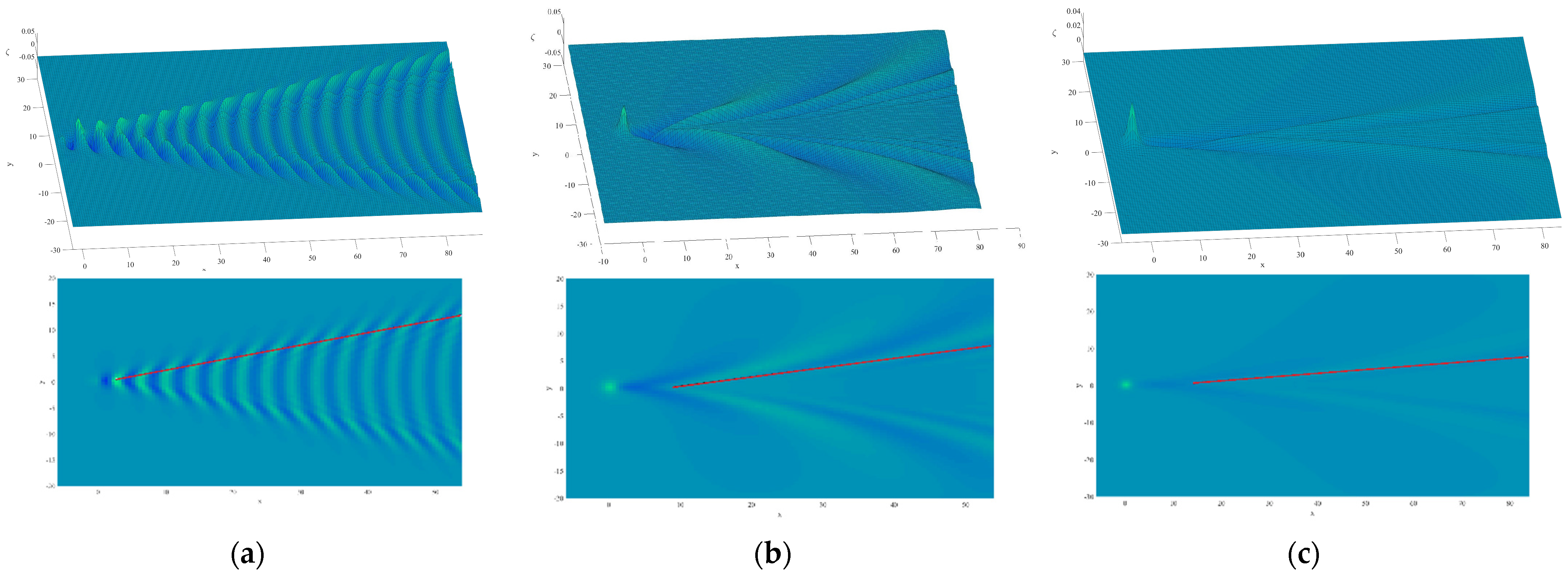
  • The ship waves have small wake angle, prominent divergent waves and long wavelength. In this case, the vessel’s overall length is short but its speed is high. In Figure 5a, there is a wake wave from the speedboat. Therefore, the Rankine source is utilized to make divergent waves conspicuous, then continuously increasing the Froude number until the wake angle is suitable. The simulation result is consistent with the real ship wave pattern.
  • The wake angles are the same as Kelvin angle, with prominent transverse waves and either the value of overall length or speed is not large, like the pilot boat in Figure 5c (note that: due to the far perspective, the entire wake pattern looks slightly smaller. However, the primary waveform is also consistent with Figure 5d). It is better to choose the Kelvin source, low source strength and the moderately small value of the Froude number. The perspective view of the pattern for   F = 0.7   and   ϵ = 0.5 is presented in Figure 5d.
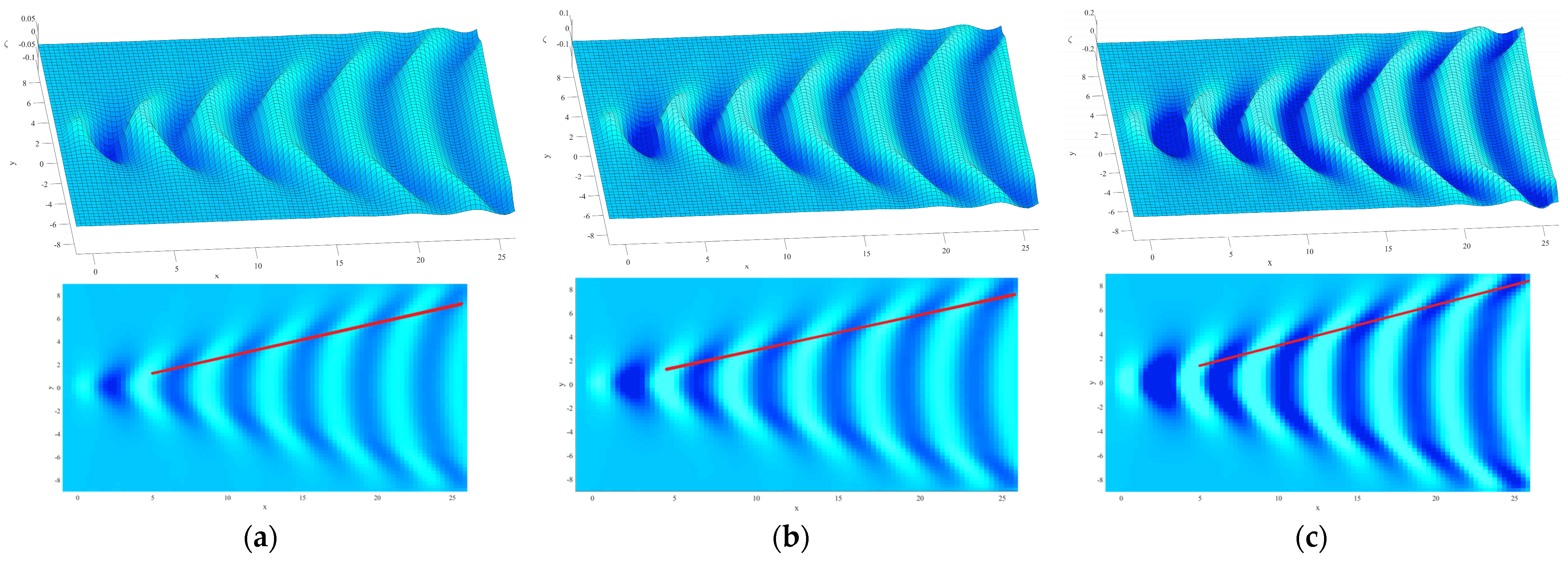
  • The ship waves have large wage angle, prominent divergent waves and short wavelength. Generally, only the large vessels can profile these wakes (Figure 5e). It is right to enhance the source strength to increase the wake angle, and then utilize the Rankine source to make the divergent waves prominent. The perspective view of the pattern for F = 0.7   and   μ = 0.5 is presented in Figure 5f.
In conclusion, the simulation method adopted in this paper can simulate the polymorphic ship waves, and the simulation results are consistent with real ship waves. Therefore, it is feasible to discuss the wake angle on that basis.

5. Discussions of Kelvin Wake Angle

In Section 4, this paper proposes the approximate variation tendency of the waveform by adjusting the parameters. Then, in this section, the wake angle is discussed for Froude number, source strength and source type in more detail.

5.1. The Effect of Froude Number on Wake Angle

To demonstrate the effect of Froude number on apparent wake angle, Figure 6 shows three free surface patterns for flow past the Rankine source, computed for F = 0.7 ,   2.5 ,   5.0 and μ = 0.4 on a 181 × 61 mesh with Δ x = 0.3 , Δ y = 0.3 . The wake angle decreases as Froude number increases. The reason is that the highest peaks do not locate in the outermost divergent under enough large Froude numbers, and then the wake angle gets smaller apparently. In Figure 6a, the Froude number is a moderately small value and the wake angle is almost the same as Kelvin angle. However, in Figure 6b,c, the wake angle is much smaller than the Kelvin angle, ending up with the wake angle and Froude approximately inversely proportional.
Therefore, we should use specific data to obtain an accurate conclusion. The wake angle θ is measured in the contour plot, whose highest peaks are easily found. As shown in Figure 7, the angle between the line connecting these peaks and the ship heading is the wake angle θ . To clearly illustrate the effect of Froude number F , this paper keeps the source strength and source type invariant, obtains a series of data of wake angles with changing Froude number and sets two groups of data for comparing. The Cartesian coordinates of F and θ . are established, as shown in Figure 8. The Froude number F ranges from 0.8 to 5.0, the trend of the wake angle θ obviously tends to decrease with Froude number. However, gradients are obviously different between the range of Froude number from 0.8 to 2.0 and the range of Froude number from 3.0 to 5.0. In the first interval, the wake angle decreases slowly with Froude number and the value of the wake angle fluctuates up and down; in the second interval, wake angle decreases dramatically with Froude number. In sum, the downtrend of the wake angle with Froude number has two stages; it is only when the Froude number reaches a threshold that the wake angle is inversely proportional to the Froude number; the threshold is independent of the source strength, around 2.0 when the Rankine source is used as a disturbance. This finding can be reflected in real situations; only when the ship speed is high enough will the transformation of wake angle be noticeable.

5.2. The Effect of Source Strength on Wake Angle

In this paper, different source strengths ϵ = 1.0 ,   1.5 ,   2.5 are utilized to generate different wave patterns for the flow past Kelvin source with F = 0.8 , as shown in Figure 9. It is well known that the Kelvin angle is 19.47°. Comparing the wake angles with the Kelvin angle, the wake angle is slightly smaller than the Kelvin angle in Figure 9a. However, the Kelvin angle in Figure 9c is larger than the Kelvin angle. Although the wake angle change is not significant, the wake angle is tending to slowly increase with the source strength. In other words, the wake angle is tending to slowly increase with the ship size.
Meanwhile, Cartesian coordinates of θ and ϵ are established by keeping Froude number and source type invariant and adjusting source strength, obtaining two sets of data with F = 0.8 . and F = 1.2 , shown in Figure 10. The source strength ϵ . ranges from 1.0 to 3.0 and the wake angle increases with the source strength. However, the two sets of data show slightly different trends. With F = 0.8 , the wake angle increases at an almost steady rate with source strength; with F = 1.2 , the wake angle barely changes as source strength increases at first, then increases at a steady rate after source strength reaching 1.8. In a word, compared with Froude number, although the source strength cannot greatly affect the wake angle, it is clear that the wake angle increases with source strength.

5.3. The Effect of Source Type on Wake Angle

The two free surface patterns for flow past the Kelvin source and Rankine source, respectively, are computed for the Froude number F = 0.8 . The amplitudes of ship waves, generated by two source types, should be adjusted to equalize. A wave profile computed for Kelvin source with ϵ = 0.9 is present in Figure 11a and the wave profile computed for the Rankine source with μ = 0.5 is given in Figure 11b. After measurement, the wake angles in the two free surface patterns are approximately equal, which means that source type does not affect the variation in wake angle. Furthermore, the wake angle has the same trend, no matter whether there is a Kelvin source or Rankine source as a disturbance. In Figure 12, there are trends of wake angle with the effect of Froude number for Kelvin source and Rankine source; both downtrends have two stages, but the first interval has a longer range in Figure 12a. The wake angle sharply decreases at Froude number 2.8 when the flow passes the Kelvin source. However, the wake angle sharply decreases at Froude number 2.0 when the flow passes the Rankine source. Therefore, the source type has an effect on the threshold about Froude number.
On the other hand, the Rankine source possesses a better capacity to avoid introducing very small spurious waves throughout the domain. Focusing on the upstream domain in Figure 11a, the spurious waves can be found, so that the whole free surface elevation is touched by spurious waves. Nevertheless, if we want to simulate the ship wave accompanied with sea clutters, introducing small spurious waves is a reasonable method.

6. Conclusions

In order to elucidate the effect of ship size on the Kelvin ship waves, this paper implements the numerical scheme, which combines the boundary integral method with the Jacobian-free Newton–Krylov method, for the simulation of nonlinear ship waves on an infinite fluid. Though imitating plenty of different Kelvin wave patterns, the mechanism of ship wave transformation is proposed, and then it is verified by comparing simulation results with real ship waves. Finally, the wake angle is discussed with the effects of Froude number, source strength and source type and the following conclusions can be drawn.
  • The wake angle tends to decrease with Froude number and the downtrend has two stages. The wake angle is inversely proportional to Froude number and decreases dramatically after Froude number reaches a threshold, which is around 2.0 for Rankine source and is around 2.8 for Kelvin source.
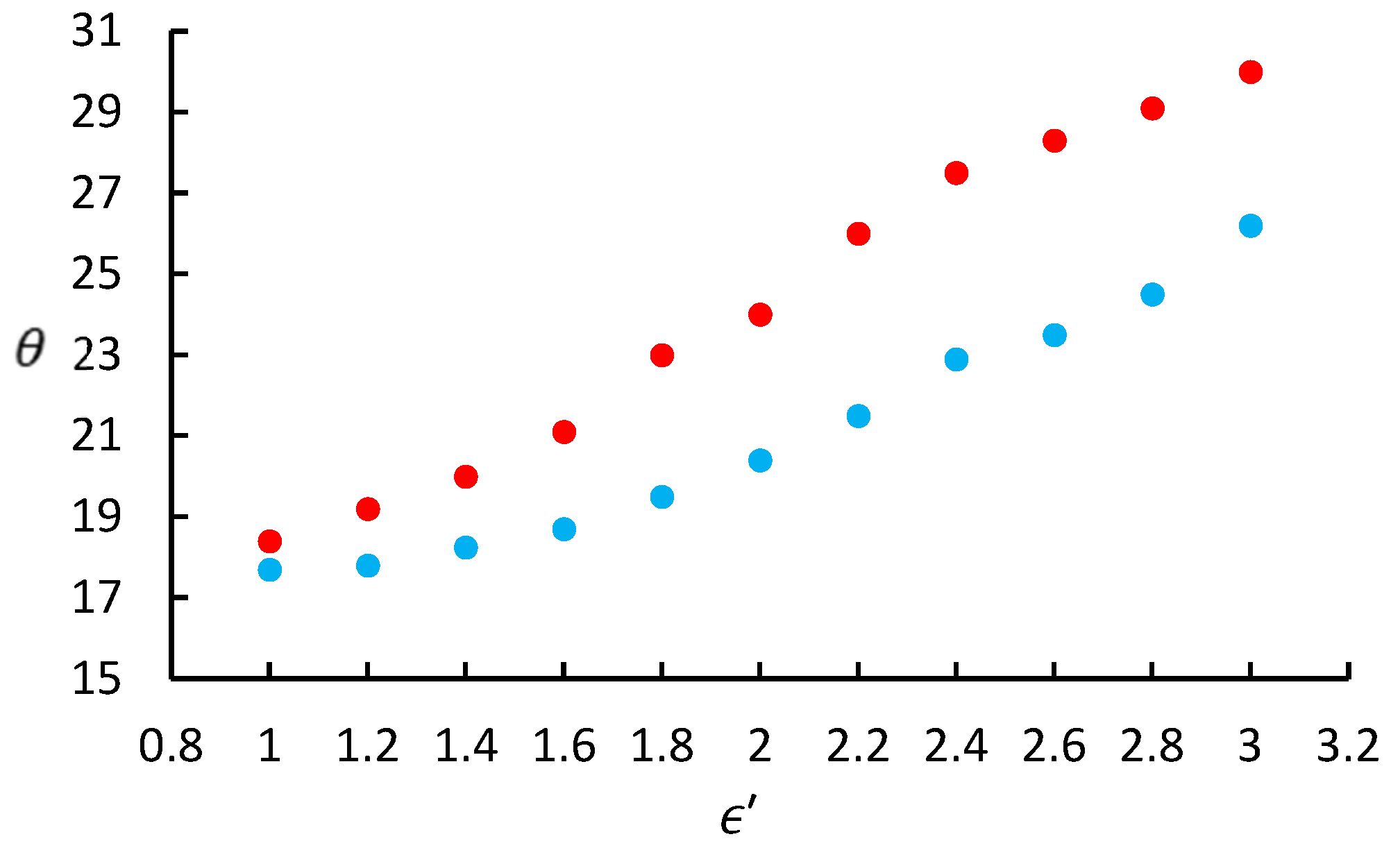
  • The wake angle tends to increase with source strength, meaning that ship size can affect the ship waves; the larger the ship size, the larger the wake angle generated will be.
  • Because the gradient of source strength is lower than the gradient of Froude number, the wake angle change caused by ship size is not as visually obvious as the ship speed. Meanwhile, it is hard for source strength to increase the wake angle when the Froude number is large.
  • With either the Kelvin source or Rankine source as a disturbance, the variation trends of wake angle are approximately identical with the effects of Froude number and source strength. However, a more accurate solution for nonlinear ship waves can be solved when the free surface flow passes Rankine source.
This paper suggests that there will be a sudden change in the downtrend of wake angle when the ship speed reaches a threshold. The next stage in research will pay attention to exploring the cause of the sudden change and investigating the influencing factors of threshold, e.g., water depth, ship shape, etc. The theoretical conclusion about threshold value will be verified by model test. This study will provide reference for informing environmentally friendly shipping policies, e.g., speed limits, etc.

Author Contributions

Conceptualization, X.S. and M.C.; methodology, X.S. and M.C.; software, M.C. and J.W.; validation, X.S. and C.L.; formal analysis, X.S., J.W. and C.L.; writing—original draft preparation, X.S. and M.C.; writing—review and editing, X.S., M.C., J.W. and C.L.; supervision, X.S. All authors have read and agreed to the published version of the manuscript.

Funding

The work was supported by the National Key Research and Development Program of China (No. 2019YFE0111600), National Natural Science Foundation of China (No. 52071049, 61971083 and 51939001), Liao Ning Revitalization Talents Program (No. XLYC2002078) and Dalian Science and Technology Innovation Fund (No. 2019J11CY015). The authors would like to express sincere thanks for their support.

Institutional Review Board Statement

Not applicable.

Informed Consent Statement

Not applicable.

Data Availability Statement

Not applicable.

Conflicts of Interest

The authors declare no conflict of interest.

Nomenclature

U Fward speed of shipnDecay coefficient of radiation condition
LThe vertical distance from source point to free surface x 1 boundary value
m, ĸKelvin source strength and Rankine source strengthF(u)The nonlinear system of equations
ϵ , μ Dimensionless Kelvin source strength and Rankine source strengthuThe vector of unknowns in the nonlinear system
F Dimensionless Froude numberJ(ut) Jacobian matrix.
Φ ( x , y , z ) ,   ϕ ( x , y ) Dimensionless velocity potential K m Krylov subspace
ζ ( x , y ) Dimensionless free surface elevationPPreconditioner matrix
P ( ρ , σ , τ ) , Q ( x , y , z ) Field pointsr0Initial linear residual
nThe downward pointing unit normal vector to the free surfaceu0Initial value of unknowns
N,MThe number of columns and rows in the meshhSmall perturbation
Δ x , Δ y The intervals in x- and y-directionsABCDSubmatrices of preconditioner matrix
ϕ x , ϕ y x-derivatives and y-derivatives of velocity potentialIUnit matrix
ζ x , ζ y x-derivatives and y-derivatives of free surface elevationosrColumn matrix in the process of solving preconditioner matrix

References

  1. Dias, F. Ship Waves and Kelvin. J. Fluid Mech. 2014, 746, 1–4. [Google Scholar] [CrossRef] [Green Version]
  2. Michell, J.H. The Wave-Resistance of a Ship. Lond. Edinb. Dublin Philos. Mag. J. Sci. 1898, 45, 106–123. [Google Scholar] [CrossRef]
  3. Sheremet, A.; Gravois, U.; Tian, M. Boat-Wake Statistics at Jensen Beach, Florida. J. Waterw. Port Coast. Ocean Eng. 2013, 139, 286–294. [Google Scholar] [CrossRef]
  4. Wang, L.; Liu, J.; Min, G.; Xie, Y. Simulation for the Ship Kelvin Wake with Narrow Components in SAR Image. In Proceedings of the 2021 Cross Strait Radio Science and Wireless Technology Conference (CSRSWTC 2021), Shenzhen, China, 13 October 2021; pp. 186–188. [Google Scholar]
  5. Pethiyagoda, R.; Moroney, T.J.; Macfarlane, G.J.; McCue, S.W. Spectrogram Analysis of Surface Elevation Signals Due to Accelerating Ships. Phys. Rev. Fluids 2021, 6, 104803. [Google Scholar] [CrossRef]
  6. Luo, Y.; Zhang, C.; Liu, J.; Xing, H.; Zhou, F.; Wang, D.; Long, X.; Wang, S.; Wang, W.; Shi, F. Identifying Ship-Wakes in a Shallow Estuary Using Machine Learning. Ocean Eng. 2022, 246, 110456. [Google Scholar] [CrossRef]
  7. Kelvin, L. On Ship Waves. Proc. Inst. Mech. Eng. 1887, 38, 409–434. [Google Scholar] [CrossRef]
  8. Lighthill, M.J. Waves in Fluids. J. Fluid Mech. 1978, 90, 605–607. [Google Scholar] [CrossRef]
  9. Rabaud, M.; Moisy, F. Ship Wakes: Kelvin or Mach Angle? Phys. Rev. Lett. 2013, 110, 214503.1–214503.5. [Google Scholar] [CrossRef]
  10. Verberck, B. Hydrodynamics: Wake Up. Nat. Phys. 2013, 9, 390. [Google Scholar] [CrossRef]
  11. Darmon, A.; Benzaquen, M.; Raphaël, E. Kelvin Wake Pattern at Large Froude Numbers. J. Fluid Mech. 2014, 738, R3. [Google Scholar] [CrossRef] [Green Version]
  12. Benzaquen, M.; Darmon, A.; Raphael, E. Wake Pattern and Wave Resistance for Anisotropic Moving Disturbances. Phys. Fluids 2014, 26, 092106. [Google Scholar] [CrossRef] [Green Version]
  13. Miao, S.; Liu, Y. Wave Pattern in the Wake of an Arbitrary Moving Surface Pressure Disturbance. Phys. Fluids 2015, 27, 122102. [Google Scholar] [CrossRef]
  14. Ma, C.; Zhu, Y.; Wu, H.; He, J.; Zhang, C.; Li, W.; Noblesse, F. Wavelengths of the Highest Waves Created by Fast Monohull Ships or Catamarans. Ocean Eng. 2016, 113, 208–214. [Google Scholar] [CrossRef]
  15. Zhu, Y.; Wu, H.; Ma, C.; He, J.; Li, W.; Wan, D.; Noblesse, F. Michell and Hogner Models of Far-Field Ship Waves. Appl. Ocean Res. 2017, 68, 194–203. [Google Scholar] [CrossRef]
  16. Wu, H.; Wu, J.; He, J.; Zhu, R.; Yang, C.J.; Noblesse, F. Wave Profile Along a Ship Hull, Short Far-Field Waves, and Broad Inner Kelvin Wake Sans Divergent Waves. Phys. Fluids 2019, 31, 47102. [Google Scholar] [CrossRef]
  17. Ellingsen, S.A. Ship Waves in the Presence of Uniform Vorticity. J. Fluid Mech. 2014, 742, R2. [Google Scholar] [CrossRef] [Green Version]
  18. Li, Y.; Ellingsen, S.A. Ship Waves on Uniform Shear Current at Finite Depth: Wave Resistance and Critical Velocity. J. Fluid Mech. 2016, 791, 539–567. [Google Scholar] [CrossRef] [Green Version]
  19. Li, Y. Wave-Interference Effects on Far-Field Ship Waves in the Presence of a Shear Current. J. Ship Res. 2018, 62, 37–47. [Google Scholar] [CrossRef]
  20. Wu, H.; He, J.; Liang, H.; Noblesse, F. Influence of Froude Number and Submergence Depth on Wave Patterns. Eur. J. Mech. B Fluids 2019, 75, 258–270. [Google Scholar] [CrossRef]
  21. Liang, H.; Chen, X. Asymptotic Analysis of Capillary–Gravity Waves Generated by a Moving Disturbance. Eur. J. Mech. 2018, 72, 624–630. [Google Scholar] [CrossRef]
  22. Grue, J. Ship Generated Mini-Tsunamis. J. Fluid Mech. 2017, 816, 142–166. [Google Scholar] [CrossRef] [Green Version]
  23. Liang, H.; Chen, X. Viscous Effects on the Fundamental Solution to Ship Waves. J. Fluid Mech. 2019, 879, 744–774. [Google Scholar] [CrossRef]
  24. Pethiyagoda, R.; Moroney, T.J.; Lustri, C.J.; McCue, S.W. Kelvin Wake Pattern at Small Froude Numbers. J. Fluid Mech. 2021, 915. [Google Scholar] [CrossRef]
  25. Havelock, T.H. Ship Waves: The Calculation of Wave Profiles. Proc. R. Soc. Lond. Ser. A Contain. Pap. A Math. Phys. Character 1932, 135, 1–13. [Google Scholar] [CrossRef] [Green Version]
  26. Wehausen, J.V.; Laitone, E.V. Surface Waves; Springer: Berlin, Germany, 1960; pp. 446–778. ISBN 978-3-642-45944-3. [Google Scholar]
  27. Barbosa, E.; Daube, O. A Finite Difference Method for 3D Incompressible Flows in Cylindrical Coordinates. Comput. Fluids 2005, 34, 950–971. [Google Scholar] [CrossRef] [Green Version]
  28. Bettess, P.; Bettess, J.A. Analysis of Free Surface Flows Using Isoparametric Finite Elements. Int. J. Numer. Methods Eng. 1983, 19, 1675–1689. [Google Scholar] [CrossRef]
  29. Forbes, L.K. On the Effects of Non-Linearity in Free-Surface Flow about a Submerged Point Vortex. J. Eng. Math. 1985, 19, 139–155. [Google Scholar] [CrossRef]
  30. Wang, H.; Zhu, R.; Gu, M.; Gu, X. Numerical Investigation on Steady Wave of High-Speed Ship with Transom Stern by Potential Flow and CFD Methods. Ocean Eng. 2022, 246, 110456. [Google Scholar] [CrossRef]
  31. Kan, Z.; Song, N.; Peng, H.; Chen, B. Extension of Complex Step Finite Difference Method to Jacobian-Free Newton–Krylov Method. J. Comput. Appl. Math. 2022, 399, 113732. [Google Scholar] [CrossRef]
  32. Ma, C.; Scheichl, R.; Dodwell, T. Novel Design and Analysis of Generalized Finite Element Methods Based on Locally Optimal Spectral Approximations. SIAM J. Numer. Anal. 2022, 60, 244–273. [Google Scholar] [CrossRef]
  33. Bystricky, L.; Pålsson, S.; Tornberg, A.K. An Accurate Integral Equation Method for Stokes Flow with Piecewise Smooth Boundaries. BIT Numer. Math. 2021, 61, 309–335. [Google Scholar] [CrossRef]
  34. Gu, M.; Zhu, R.; Yang, X.; Wang, H.; Shi, K. Numerical Investigation on Evaluating Nonlinear Waves Due to an Air Cushion Vehicle in Steady Motion by a Higher Order Desingularized Boundary Integral Equation Method. Ocean Eng. 2022, 246, 110598. [Google Scholar] [CrossRef]
  35. Forbes, L.K. An Algorithm for 3-Dimensional Free-Surface Problems in Hydrodynamics. J. Comput. Phys. 1989, 82, 330–347. [Google Scholar] [CrossRef]
  36. Pethiyagoda, R. Mathematical and Computational Analysis of Kelvin Ship Wave Patterns. Ph.D. Thesis, Queensland University of Technology, Brisbane, Australia, 2016. [Google Scholar]
  37. Scullen, D.C. Accurate Computation of Steady Nonlinear Free-Surface Flows. Ph.D. Thesis, The University of Adelaide, Adelaide, Australia, 1998. [Google Scholar]
  38. Brown, P.N.; Saad, Y. Hybrid Krylov Methods for Nonlinear Systems of Equations. SIAM J. Sci. Stat. Comput. 1990, 11, 450–481. [Google Scholar] [CrossRef]
  39. Saad, Y.; Schultz, M.H. GMRES: A Generalized Minimal Residual Algorithm for Solving Nonsymmetric Linear Systems. SIAM J. Sci. Stat. Comput. 1986, 7, 856–869. [Google Scholar] [CrossRef] [Green Version]
  40. Knoll, D.A.; Keyes, D.E. Jacobian-Free Newton-Krylov Methods: A Survey of Approaches and Applications. J. Comput. Phys. 2004, 193, 357–397. [Google Scholar] [CrossRef] [Green Version]
  41. Dembo, R.S.; Eisenstat, S.C.; Steihaug, T. Inexact Newton Methods. SIAM J. Numer. Anal. 1982, 19, 400–408. [Google Scholar] [CrossRef]
Figure 1. Illustration of the disposition about the fluid.
Applsci 12 06265 g001
Figure 2. Schematic diagram of the fluid volume and its bounding surface.
Applsci 12 06265 g002
Figure 3. Illustration of the discrete unknowns at an N × M mesh, the left black dots are the locations of ϕ and ζ , the congruent triangles are the locations of the ϕ x and ζ x .
Applsci 12 06265 g003
Figure 4. Perspective view of the free surface using Ranking source, for the case F = 0.7   and   μ = 0.3 , computed on a 151 × 51 mesh with Δ x   =   0.3 ,   Δ y   =   0.3 .
Applsci 12 06265 g004
Figure 5. Comparisons between the three types of real ship waves and the corresponding simulation results. The pictures of real ship wave patterns come from internet: (a) speedboat wake, from https://commons.wikimedia.org/wiki/File:Fjordn_surface_wave_boat.jpg accessed on 5 January 2022; (c) pilot boat wake, from https://www.shutterstock.com/zh/image-photo/small-ferry-boat-route-mainland-during-1706813791 accessed on 1 May 2022; (e) large vessel wake, from https://www.istockphoto.com/photo/aerial-top-view-oil-ship-tanker-full-speed-transportation-oil-from-refinery-on-the-gm1159334567-316959177 accessed on 5 January 2022.
Applsci 12 06265 g005
Figure 6. Perspectives and plans view of the free surfaces past Ranking source, computed on a 181 × 61 mesh with Δ x = 0.3 , Δ y = 0.3 , for the cases μ = 0.4 : (a) F = 0.7 , (b) F = 2.5 , (c) F = 5.0 . The top three free surface patterns are the perspectives and the bottom three free surface patterns are the plans. The red line marks the edge of the wake angle in each plan view.
Applsci 12 06265 g006
Figure 7. A contour plot of the nonlinear free surface profile for flow past the Rankine source with the Froude number F = 1.0 and the source strength μ = 1.0 , computed on a 181 × 61 mesh with Δ x = 0.3 , Δ y = 0.3 .
Applsci 12 06265 g007
Figure 8. A plot of apparent wake angle θ against Froude number F . for a flow past the Rankine source, with the source strength μ = 1.0 (the red circles) and μ = 0.5 (the blue circles). The black solid lines are the trendlines of the wake angles with Froude numbers.
Applsci 12 06265 g008
Figure 9. Perspectives and plans view of the free surfaces past Kelvin source, computed for the cases F = 0.8 : (a) ϵ = 1.0 , (b) ϵ = 1.5 , (c) ϵ = 2.5 . The top three free surface patterns are the perspectives and the bottom three free surface patterns are the plans. The red line marks the edge of the wake angle in each plan view.
Applsci 12 06265 g009
Figure 10. A plot of apparent wake angle θ against Froude number ϵ for a flow past the Kelvin source, with the source strength   F = 0.8 (the red circles) and F = 1.2 (the blue circles).
Applsci 12 06265 g010
Figure 11. Perspectives and plans view of the free surface computed for F = 0.8: (a) Kelvin source with ϵ = 0.9 ; (b) Rankine source with μ = 0.5 . The top two free surface patterns are the perspectives and the bottom two free surface patterns are the plans. The red line marks the edge of the wake angle in each plan view.
Applsci 12 06265 g011
Figure 12. Measured apparent wake angles θ in degrees plotted against the Froude number for the flow past a Kelvin source with ϵ = 1 (a) and a Rankine source with μ′ = 0.5 (b).
Applsci 12 06265 g012
Publisher’s Note: MDPI stays neutral with regard to jurisdictional claims in published maps and institutional affiliations.

