An fMRI Sequence Representation Learning Framework for Attention Deficit Hyperactivity Disorder Classification

Abstract

For attention deficit hyperactivity disorder (ADHD), a common neurological disease, accurate identification is the basis for treatment. In this paper, a novel end-to-end representation learning framework for ADHD classification of functional magnetic resonance imaging (fMRI) sequences is proposed. With such a framework, the complexity of the sequence representation learning neural network decreases, the overfitting problem of deep learning for small samples cases is solved effectively, and superior classification performance is achieved. Specifically, a data conversion module was designed to convert a two-dimensional sequence into a three-dimensional image, which expands the modeling area and greatly reduces the computational complexity. The transfer learning method was utilized to freeze or fine-tune the parameters of the pre-trained neural network to reduce the risk of overfitting in the cases with small samples. Hierarchical feature extraction can be performed automatically by combining the sequence representation learning modules with a weighted cross-entropy loss. Experiments were conducted both with individual imaging sites and combining them, and the results showed that the classification average accuracies with the proposed framework were 73.73% and 72.02%, respectively, which are much higher than those of the existing methods.

1. Introduction

Attention deficit hyperactivity disorder (ADHD) is a common childhood disease with neurodevelopmental and mental disorders [1], and it is characterized by a lack of sustained attention, high impulse, and hyperactivity. ADHD disease involves the influence of environmental, neurological, and genetic factors as well. The neural mechanism of ADHD disease is incompletely known, and the traditional diagnosis still depends on the analysis of clinical interviews and patients’ behaviors. There is a significant challenge to this diagnosis method, which is that the diagnosis is based on subjective behavioral criteria and this process is time-consuming. In addition, it requires in-depth domain knowledge. As human brains are similar with a large complex network that controls and monitors the whole body’s system, researchers are attempting to explore the mechanism of brain nerve diseases and diagnose them objectively by studying brain activities. In brain function research, brain functional imaging technology is commonly used to provide insight into the neural mechanism of cognition and emotion. In recent years, many different imaging methods have been applied to research on brain functional activities, such as electroencephalogram, magnetoencephalogram, and functional magnetic resonance imaging (fMRI). fMRI is a new neuroimaging method based on the blood-oxygen-level-dependent (BOLD) imaging principle, and it is also a non-invasive imaging technology that has the characteristic of the accurate positioning of brain functional activation areas. Therefore, fMRI is considered to be the most suitable brain function imaging for determining the functional activities of brain regions.

The accurate identification of ADHD will contribute to the early treatment and targeted treatment of the disease. In recent years, many achievements have been made in the classification of brain neurological diseases based on fMRI imaging and machine learning. The representation of data is one of the key parts of machine learning, data mining, and other fields, as its performance affects the achievable efficiency significantly. The structure of the human brain is complex, and the neurons in various functional brain areas interact with each other. At present, the classification of ADHD is generally based on the functional connectivity between brain regions for feature extraction and support vector machine (SVM) [2] for classification. Traditional neuroimaging data classification usually requires several preprocessing steps, such as subject selection, feature extraction, and feature selection. These steps require a large amount of domain knowledge and many skilled selection methods and will bring about the problem of experimental reproducibility [3,4].

Currently, representation learning, known as feature learning, based on deep neural networks (DNNs), has become a hot spot. The representation learning method does not need explicit data transformation, and the internal representation of data can be learned implicitly as well. Deep learning (DL) implements layer-by-layer representation transformation on massive amounts of training data by constructing a DNN with multiple hidden layers. On the other hand, automatically learned data representation has a strong description ability. Hence, with the support of extraordinary computing power, massive data, and complex models, the DL method has been successfully applied to image processing, speech recognition, intelligent search, and other fields with large amounts of training data.

However, for practical applications constrained by time, environment, and other limitations, it is usually difficult to obtain large-scale data. Generally, the sample sizes of most fMRI data sets are relatively small. In the case of a few training samples, DL has the risk of easy overfitting, and the effectiveness of the algorithm will be significantly reduced. As a result, existing DL algorithms that have excellent performance in cases where there is a large number of samples are not suitable for image analysis and processing with only a small number of samples.

To tackle the issue that large samples are needed in a DL algorithm while the number of ADHD samples is usually small, a novel end-to-end fMRI sequence representation learning framework for ADHD classification is proposed. In the proposed framework, three main innovations of this method are involved: (1) through the data conversion module, the two-dimensional sequence is converted into a three-dimensional image, which not only expands the modeling area of the adjacent regions of interest (ROIs) for the subsequent convolution operation but also greatly reduces the computational complexity of this algorithm; (2) aimed at the problem of a few ADHD samples, the transfer learning method is used to freeze or fine-tune the parameters of the pre-trained neural network for reducing the risk of overfitting; and (3) our representation learning framework can automatically perform hierarchical feature extraction, where combining the sequence representation learning modules with a weighted cross-entropy loss at the low level and high level can capture the activity characteristics of regions and the relations among them. Furthermore, this framework does not use traditional data augmentation for deep learning and complex representation selection technology. Hence, it is simple, effective, and easily applied for the diagnosis of other brain nerve diseases as well.

2. Related Work

Being one of the key parts of ADHD classification, much work has been conducted on the representation extraction of fMRI data, which can be divided into two categories, namely hand-crafted feature methods and automatic representation learning methods by deep learning.

2.1. Hand-Crafted Feature Methods

Traditional classification methods of neuroimaging data are usually based on hand-crafted features. Functional connectivity between brain regions is a representation of fMRI signals. Researchers have proposed different calculation methods for functional connectivity, among which the correlation of different brain regions is the most common one. In [5], the research team at Yale University proposed the functional connectome method to calculate the correlation coefficient for the BOLD signal sequence of the ROIs in the whole brain, and then a connection matrix was constructed as the representation of interregional connectivity, which can be effectively applied to behavior prediction, such as memory and emotion tasks. In [6], Riaz et al. proposed a novel scheme to learn the functional connectivity of two brain regions through a similarity measurement network. In addition to structural MRI data and fMRI data, the fusion of phenotypic information, such as gender, age, and IQ, can improve classification accuracy [7]. Khan et al. proposed a knowledge distillation and representation selection method for ADHD classification in [8].

In general, a hand-crafted feature method for fMRI data usually includes feature extraction, feature selection, etc., which require exquisite design skills and in-depth domain knowledge of brain neuroscience.

2.2. Representation Learning Methods

Recent DL has a very good performance in many kinds of application fields. DL can implement layer-by-layer representation transformation on massive training data by constructing a DNN with multiple hidden layers, and its algorithm is good at dealing with highly complex data that may interact in a highly nonlinear way at multiple levels. On the other hand, the automatically learned-based data representation has a strong description ability. DL can automatically learn relevant high-level representations from raw data, which makes DL successfully be applied in the biomedical field [9]. When it is applied to some medical fields with a large amount of data, DL has great potential. Therefore, there is a growing trend to apply representation learning in biology [10]. DNNs have successfully been applied to the automatic detection of skin cancer and breast cancer [11,12]. The DeepMind company proposed an AlphaFold system based on a DNN for protein structure prediction [13]. In [14], Ji et al. proposed convolutional kernels with an element-wise weighting mechanism to extract deep features of the functional connectome. In [15], Riaz et al. proposed an end-to-end DeepFMRI framework for ADHD classification that consists of a feature extraction network, a function connection network, and a classification network. In [16], Zhang et al. proposed a method of combining a convolutional neural network with attention to identify ADHD.

3. Materials and Methods

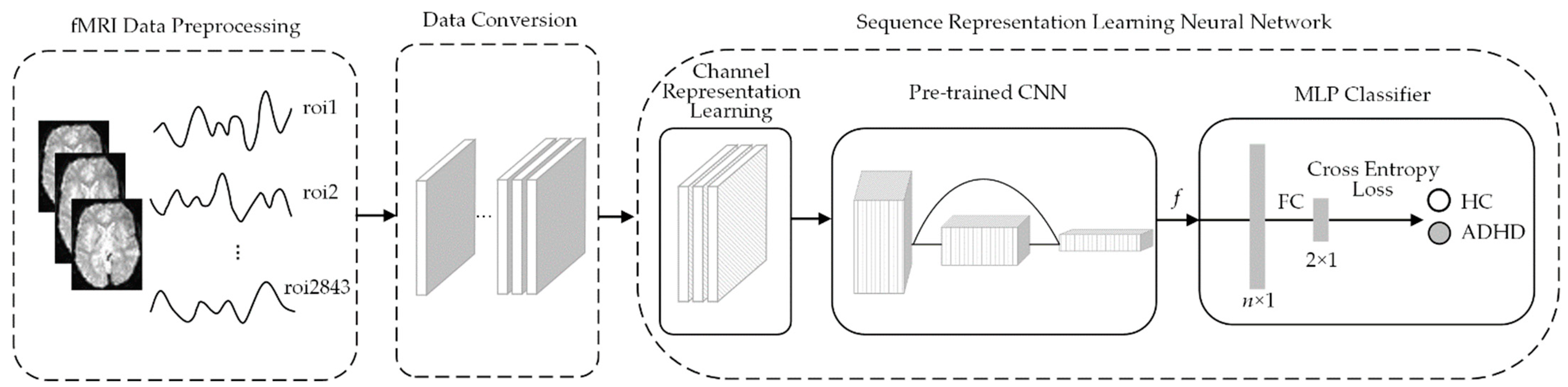
In this paper, an end-to-end fMRI sequence representation learning framework is proposed for ADHD classification. This framework is illustrated in Figure 1, and three main parts are involved: an fMRI data preprocessing module, a data conversion module, and a sequence representation learning neural network. The operation of the sequence representation learning neural network involves three steps. Firstly, the channel representation learning module uses a 1 × 1 × s convolution operation to extract the low-level features of the sequence. Then, the pre-trained neural network based on the transfer learning method is used to extract the high-level features of the sequence. Finally, the classification of healthy control (HC) and ADHD is realized by multi-layer perceptron (MLP).

3.1. Data Sets

In this paper, the experimental data came from the published Neuro Bureau ADHD-200 data set (ADHD-200 sample) [17], where the data were collected from eight independent imaging sites, including 947 individuals, and the collected information includes structural MRI data, resting fMRI data, age, gender, IQ, hand habits, and other phenotypic information. According to the American Psychiatric Association 1994 standard, ADHD in these data sets is divided into three subtypes: inattention subtype, hyperactive impulse subtype, and complex subtype. In this paper, the three subtypes are uniformly called ADHD, and binary classification experiments for HC and ADHD were carried out. Meanwhile, ADHD-200 also provides benchmark test data of six imaging sites for competition.

To facilitate comparison with current mainstream methods, this study only used five data sites: Kennedy Krieger Institute (KKI), NeuroImage Sample (NI), New York University Child Study Center (NYU), Oregon Health and Science University (OHSU), and Peking University (Peking). In these five imaging sites, both training data sets and benchmark test data sets are included. The statistical data of each imaging site used in our experiments are shown in

Table 1. Overview of the data sets used in this study.

Imaging Site	Training Set						Benchmark Test Set
	Age	Female	Male	HC	ADHD	Subtotal	Age	Female	Male	HC	ADHD	Subtotal
KKI	8–13	37	45	60	22	82	8–12	1	10	8	3	11
NI	11–22	17	31	23	25	48	13–26	13	12	14	11	25
NYU	7–18	75	140	98	118	216	7–17	13	28	12	29	41
OHSU	7–12	36	43	42	37	79	7–12	17	17	28	6	34
Peking	8–17	50	144	116	78	194	8–16	18	32	27	23	50
Total	-	215	403	339	280	619	-	62	99	89	72	161

. The training data set provided by the Peking imaging site included three subsets, Peking_1, Peking_2, and Peking_3, and the sample numbers for these three subsets were 85, 67, and 42, respectively. In addition, some imaging sites collect multiple operation data for one participant, while some imaging sites only collect one operation datum for a single participant; therefore, only data named run1 were used in our experiment. In the training set of the NYU imaging site, one participant was not marked by gender. Therefore, the sum of the female and male training samples from the NYU site is 215, which is 1 less than the total samples 216. It can be seen from Table 1 that the number of samples in the ADHD-200 dataset is small and the samples are imbalanced.

The number of subjects, scanning parameters, and equipment used varied across these different imaging sites. Detailed information about fMRI data acquisition parameters and instructions is available in Table 3 in [18]. For example, when the fMRI instrument was scanning, the participants in the NI and NYU sites were asked to keep their eyes closed, the participants in the KKI and OHSU sites were asked to keep their eyes open and fixate on an image, and the participants in Peking site were asked to keep their eyes closed or fixate. The variations in these imaging sites, as described above, lead to the heterogeneity of fMRI data, which increases the difficulty of ADHD classification.

3.2. fMRI Data Preprocessing

It is very complex to preprocess the original fMRI data. In order to encourage researchers in statistics, computer science, and other fields to use the data set, three forms of preprocessed data are provided on the NITRC platform for direct download [18,19]. These three preprocessing methods are Athena, Burner, and NIAK. The NIAK preprocessing pipeline [20] was used in this paper. NIAK preprocessing includes slice time correction, motion correction, spatial normalization of anatomical structure image, coregistration, extraction of mean/std/mask for functional images, correction of slow time drifts, correction of physiological noise, resampling of functional data, and spatial smoothing.

The original fMRI data were four-dimensional data including three dimensions in space (i.e., x, y, and z) and one dimension in time. The brain was divided into small three-dimensional voxels or regions, and the activity records for each region formed a time series. The NIAK preprocessing used the region-growing algorithm to generate functional brain parcellations, and the original four-dimensional fMRI data were converted into two-dimensional time series, which represented the signal value of each ROI at a certain time point. Then, the preprocessed fMRI data become a sequence of multiple ROIs, $X_{TS}=[x_1,x_2,\dots ,x_m]$, where m is the number of ROIs, $x_i={[a_{1i},a_2{}_i,\dots ,a_{si}]}^T$ is the sequence of the ith ROI, s is the length of the sequence, and X_TS can be expressed as a two-dimensional matrix:

$$X_{TS}=\left[\begin{array}{l}{a}_{11}{a}_{12}\dots a_{1m}\\ a_{21}{a}_{22}\dots a_{2m}\\ \dots \\ a_{s1}{a}_{s2}\dots a_{sm}\end{array}\right]$$

(1)

The NIAK pipeline provides ROI sequences with two different resolutions, namely ROI1000 and ROI3000. The ROI3000 data set was used in our experiment, where 2843 (near to 3000) ROIs were generated by setting the brain region segmentation threshold to 330 mm³.

3.3. Data Conversion

In traditional fMRI classification methods, a two-dimensional correlation coefficient matrix is often established by calculating the Pearson correlation coefficient of the time series between two ROIs, and then the correlation coefficient matrix or its upper/lower triangular matrix is generated for further classification processing. As we know, convolutional neural networks (CNNs) have been successfully applied to image classification, image segmentation, and other fields, and it can also be used to model local neighborhood relations. However, if the convolution operation is directly performed on the preprocessed fMRI two-dimensional sequence X_TS, the convolution kernel 3 × 3 can only establish the relationships among three time-step sequences and three adjacent ROIs. Therefore, the modeling area is too small.

The data conversion module was introduced to convert the two-dimensional sequence matrix, X_TS, into a three-dimensional image X_IMG. As shown in Equation (1), the one-dimensional vector [a_j1, a_j2, …, a_jm], noted as v_j, represents the signal values of m ROIs at the jth time point. Hence, according to the row-first method, the vector, v_j, can be transformed into a two-dimensional matrix, b_j, with a size of r × r by a reshaping function, where r = $\lceil \sqrt{m}\rceil$ and the insufficient bits are filled with 0. Therefore, the preprocessed fMRI two-dimensional sequence, X_TS, composed of vectors v_j (j = 1, 2, …, s) at s time points, can be converted into a three-dimensional image X_IMG of r × r × s, which is stacked by s two-dimensional matrices b_j (j = 1, 2, …, s) according to the time axis. 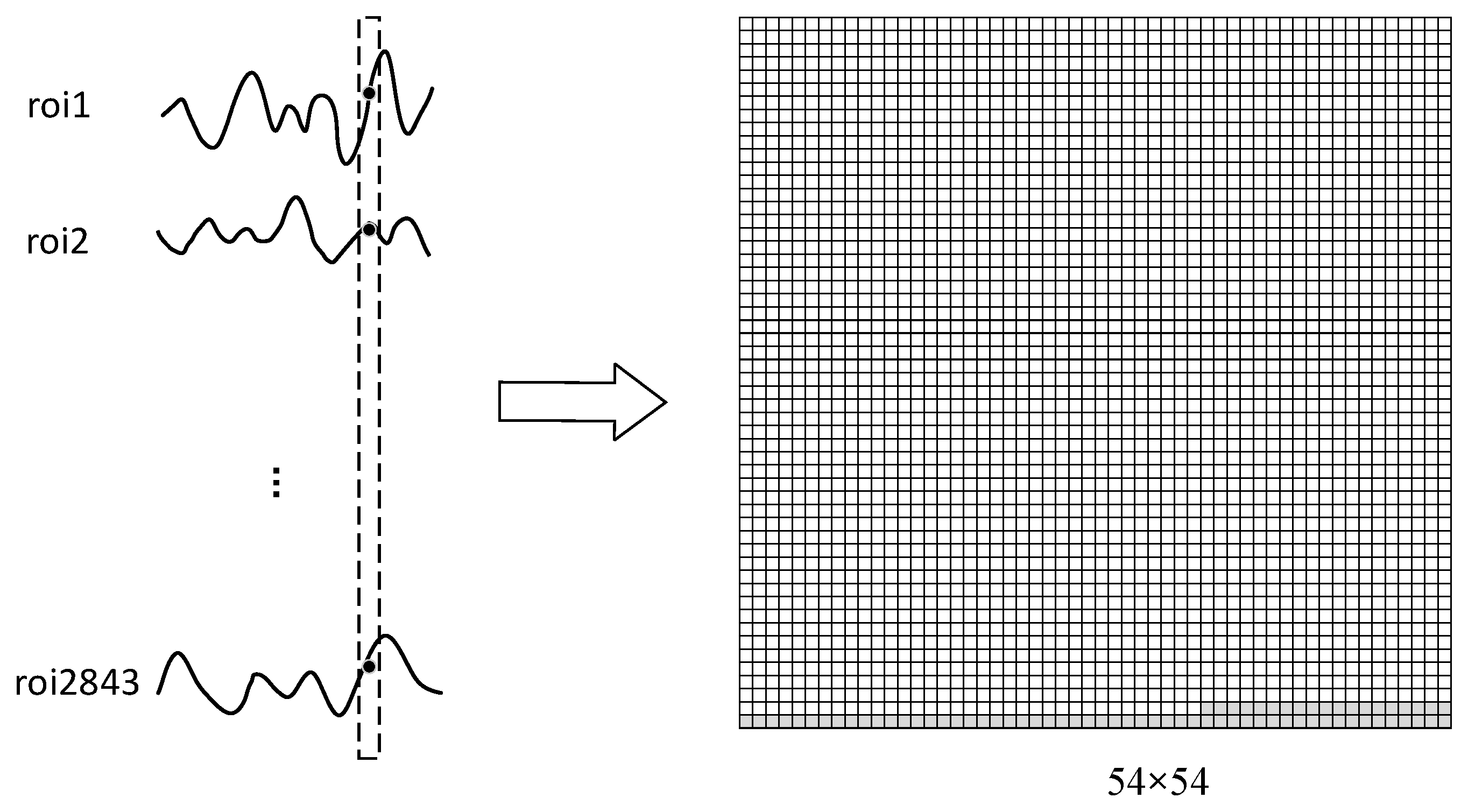Obviously, the third dimension of the three-dimensional image X_IMG is the same as the second dimension of the two-dimensional sequence X_TS, which refers to the time dimension. A diagram of the data conversion is presented in Figure 2. The specific conversion method was as follows: the BOLD values of all 2843 ROIs at a time point in the dotted box on the left were converted into a two-dimensional image of 54 × 54 on the right.

3.4. Sequence Representation Learning Neural Network

The proposed sequence representation learning neural network includes a channel sequence representation learning module, a pre-trained convolutional neural network, and an MLP classifier. They are detailly deduced in following.

3.4.1. Channel Sequence Representation Learning Module

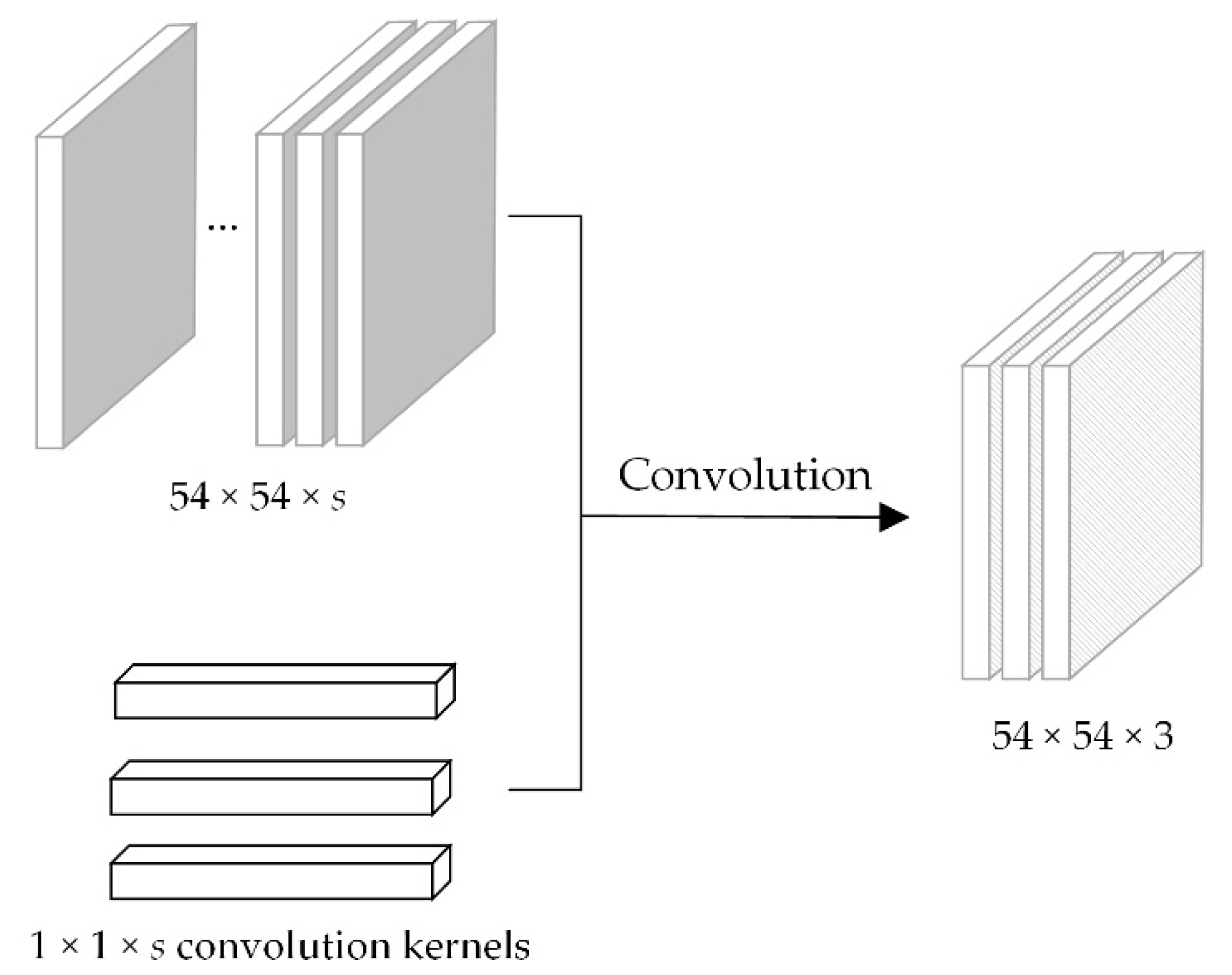
The channel sequence representation learning module extracts the channel sequence representations of the fMRI data by operating convolution with a 1 × 1 × s kernel on the three-dimensional image, X_IMG. This module can effectively capture the discriminative low-level representations from different ROIs. The number of channels of three-dimensional image X_IMG is s. Among the five imaging sites involved in this experiment, the value of s was between 73 and 257. Because the output of the channel sequence representation learning module was used as the input of the pre-trained neural network in the next module and also considering the fact that the number of input channels of the commonly pre-trained neural network is generally 3, it was necessary to compress the number of channels, s, into 3, where the three-dimensional image of h × w × s was converted into the three-dimensional image of h × w × 3. The diagram of the channel sequence representation learning module is shown in Figure 3.

3.4.2. Pre-trained Convolutional Neural Network

Our method uses a pre-trained CNN for automatic representation extraction. Brain neurons in various functional regions interact with each other, which results in a complex internal correlation of the original fMRI data. CNN is one of the most popular neural networks. It has the characteristics of local connection and weight sharing [21]. Based on its local connection characteristics, CNN can capture the brain neuron interaction patterns between various ROIs. The parameter weight-sharing mechanism greatly reduces the number of parameters of neural network. The sample size of fMRI data is usually small. Hence, when the CNN network is operated on fMRI data, overfitting will occur if a network is trained from scratch. Therefore, the pre-trained CNN model was used in our model based on transfer learning, which can transfer knowledge to a new environment.

Generally, the layers of the neural network are deeper, and the representation ability of the model is higher, but the gradient of the deep network may disappear. To overcome this drawback, the Residual Network (ResNet) [22] with identity mapping was proposed by He et al. Based on a plain network, the ResNet is built by inserting a shortcut connection between two convolution layers. ResNet has many structures with varying depths, such as 18, 34, 101, and 152. ResNet34 network mainly contains 33 convolutional layers and a fully connected layer. When ResNet34 was used as a pre-trained neural network for the representation learning of this framework, its last fully connected layer should be removed. The length of the extracted high-level representation vector is 512.

ResNet performs well in many computer vision tasks. Therefore, it has become a classic backbone applied to the construction of various types of neural networks. The pre-trained ResNet model trained on the large-scale ImageNet dataset has been successfully applied for many scenarios. There are a number of ResNet models that can be chosen, which include ResNet18, ResNet34 and ResNet101. Considering complexity and performance, in the experiments we conducted in this study, we chose the ResNet34 model, which showed satisfactory performance with moderate complexity.

3.4.3. MLP Classifier

For binary classification problems, neural networks often use a fully connected (FC) layer and a SoftMax activation function to build a trainable MLP classifier. As shown in Figure 1, after the image representation f is extracted at the last layer of the pre-trained neural network, it is sent to the MLP classifier to classify HC and ADHD. Let the length of image representation f be n, and the FC in the MLP classifier maps an n-dimensional representation vector f to a two-dimensional vector y, where each dimension of y corresponds to one category. This model uses cross-entropy as the loss function of representation learning neural network. The cross-entropy can be calculated as:

$$L=-\frac{1}{k}{\displaystyle \sum _{i=1}^k\left[y_i\log ({\widehat{y}}_i)+(1-y_i)\log (1-{\widehat{y}}_i)\right]}$$

(2)

where k is the number of samples, y_i is the expected output category of samples, and ${\widehat{y}}_i$ is the actual output category of samples. Cross-entropy is used to describe the distance between the actual output and the expected output. When the probability distribution of the actual output and the expected output is closer, the value of cross-entropy is smaller, and vice versa. The cross-entropy loss function evaluates the prediction of individual samples and then averages the results of all samples.

If the samples are imbalanced, the value of cross-entropy is dominated by the category with a large number of samples, which is disadvantageous to classification. Using the weighted cross-entropy loss function can solve the problems caused by sample imbalance to a certain degree. The weighted cross-entropy loss function, L_α, is defined as:

$$L_{\alpha }=-\frac{1}{k}{\displaystyle \sum _{i=1}^k\left[\alpha y_i\log ({\widehat{y}}_i)+(1-y_i)\log (1-{\widehat{y}}_i)\right]}$$

(3)

where α is the weight. In ADHD classification, the number of ADHD samples is less than the number of HC samples and, generally, α is set to be greater than 1, indicating that increasing the weight of ADHD samples can reduce missed diagnoses.

3.5. Evaluation Metrics

For the binary classification problem, the samples can be divided into true positive (TP) cases, false positive (FP) cases, true negative (TN) cases, and false negative (FN) cases according to the combination of their real categories and prediction categories, where TP represents the number of samples in which positive cases are correctly predicted to be positive, TN represents the number of samples in which negative cases are correctly predicted to be negative, FP represents the number of samples in which negative cases are incorrectly predicted to be positive, and FN represents the number of samples in which positive cases are incorrectly predicted to be negative. There are many evaluation metrics to evaluate the ADHD classification performance.

Accuracy (ACC) is the most common classification evaluation metric, which is the number of correctly classified samples divided by the number of all samples. It is measured as in Equation (4). Generally speaking, the higher the accuracy, the better the classifier.

$$ACC=\frac{TP+TN}{TP+TN+FP+FN}$$

(4)

Sensitivity (SEN) refers to the proportion of correctly identified positive cases in all positive cases, which is shown in Equation (5). High sensitivity means a low missed diagnosis rate.

$$SEN=\frac{TP}{TP+FN}$$

(5)

Specificity (SPC) refers to the proportion of correctly identified negative cases in all negative cases, which is shown as Equation (6). High specificity means a low misdiagnosis rate.

$$SPC=\frac{TN}{TN+FP}$$

(6)

4. Results

Five ADHD classification experiments were performed on data from five imaging sites. Our experiments adopted the PyTorch framework, and the graphics card was GeForce GTX1050.

4.1. Experimental Setup

In our experiments, imaging sites’ data are taken from KKI, NI, NYU, OHSU, and Peking of ADHD-200. The time sequence length of the data for each imaging site was different, among which the time sequence length of OHSU was the shortest, and its value was 73. The deep learning network requires a fixed length of an input signal. Therefore, all experiments only took the front part sequence of each imaging site’s data, and the time sequence length s was set to 73.

An end-to-end fMRI sequence representation learning framework was constructed to classify ADHD, which is shown in Figure 1. Specifically, the preprocessed fMRI data, a sequence of multiple ROIs, X_TS, was firstly passed to the data conversion module, where X_TS was converted into X_IMG by a reshaping function. Then, the three-dimensional image, X_IMG, was fed into the channel sequence representation learning module, which was a convolutional layer with three 1 × 1 × s kernels. Next, it was connected by the pre-trained CNN, which produced the image feature f as output and was followed by a rectified linear unit (ReLU). Finally, the feature f was sent to the MLP classifier to classify HC and ADHD. The MLP classifier was composed of a fully connected layer and an activation layer. The training of the representation learning neural network needs to set up a loss function, an optimizer, and so on. ResNet34 is used as the pre-trained CNN in our model. The nn.crossentropyloss() function of the torch library was used as a loss function, where this cross-entropy is a negative log-likelihood loss function based on the log transformation of the SoftMax() activation function, and weight α equals 2 or 3. During the neural network training, the batch size of the samples was set to 32, the learning rate lr was 3 × 10⁻⁵, the number of epochs was 14, and the Adam optimization method was adopted. In the experiments, the following two schemes commonly used in ADHD classification were taken: (1) training and test on individual imaging site data and (2) training on combining site data and test on individual benchmark test data.

4.2. Classification Experiment of Training and Test on Individual Imaging Site Data

Each of the five imaging sites (i.e., KKI, NI, NYU, OHSU, and Peking) had a training set and benchmark test set. The ADHD classification experiment of the training and test on individual imaging site data, individual site experiment for short, refers to the training data using the training set of a single imaging site and the test data using the benchmark test set of this same imaging site. During the training of the representation learning neural network, all of the parameters of the pre-trained neural network in the individual site experiment were frozen, which was mainly based on two considerations. On the one hand, it can alleviate the overfitting problem of the deep neural network with a small number of training samples; on the other hand, by freezing all of the parameters of the pre-trained neural network, verifying the applicability of the proposed method can be focused on. In the individual site ADHD classification experiments, the weight α in the cross-loss function was set to 3.

Table 2. Classification accuracies (%) comparison of different methods in the individual site experiments.

Method	KKI	NI	NYU	OHSU	Peking	Average
Dey et al. (2014) [1]	54.55	48	-	82.35	58.82	60.93
Fusion of fMRI and non-imaging data (2018) [7]	81.8	-	60.9	-	64.7	69.1
DeepFMRI (2020) [15]	-	67.9	73.1	-	62.7	67.9
Knowledge distillation-based (2021) [8]	60	70	73.3	71	73,3	69.52
Our proposed method	81.82	64	80.49	82.35	60	73.73

shows the comparison of the ADHD classification results of different methods in the individual site experiments, where the last column is the average classification accuracies. It can be seen from Table 2 that our method achieved the best results with KKI, NYU, and OHSU, reaching a state-of-the-art performance with an average accuracy of 73.73%.

To evaluate the proposed method more comprehensively, other performance metrics, such as specificity and sensitivity, had also been exploited on all five imaging sites. To compare with the existing methods, all the results with our proposed method in the individual site experiments are presented in

Table 3. The specificity (%), sensitivity (%), and accuracy (%) comparison of different methods in the individual site experiments.

Evaluation Metrics	Methods	KKI	NI	NYU	OHSU	Peking
Specificity	Dey et al. (2014) [1]	62.5	64.29	-	89.29	92.59
	Fusion of fMRI and non-imaging data (2018) [7]	75.0	42.8	41.6	-	92.6
	DeepFMRI (2020) [15]	-	71.4	91.6	-	79.1
	Our proposed method	87.5	71.43	75	92.86	59.26
Sensitivity	Dey et al. (2014) [1]	33.33	27.27	-	50.00	20.83
	Fusion of fMRI and non-imaging data (2018) [7]	100	45.4	68.9	-	33.3
	DeepFMRI (2020) [15]	-	63.6	65.5	-	48.1
	Our proposed method	66.67	54.55	82.76	33.33	60.87
Accuracy	Dey et al. (2014) [1]	54.55	48	-	82.35	58.82
	Fusion of fMRI and non-imaging data (2018) [7]	81.8	44	60.9	-	64.7
	DeepFMRI (2020) [15]	-	67.9	73.1	-	62.7
	Our proposed method	81.82	64	80.49	82.35	60

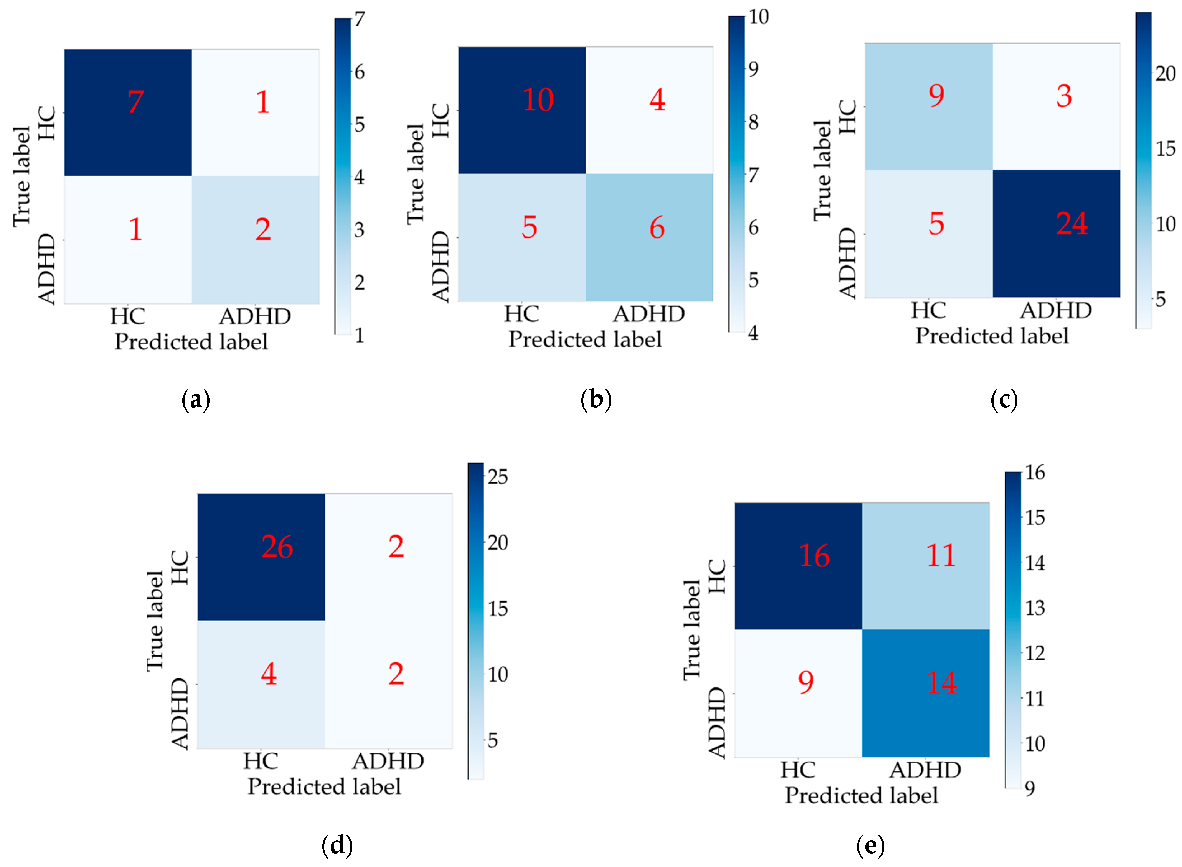
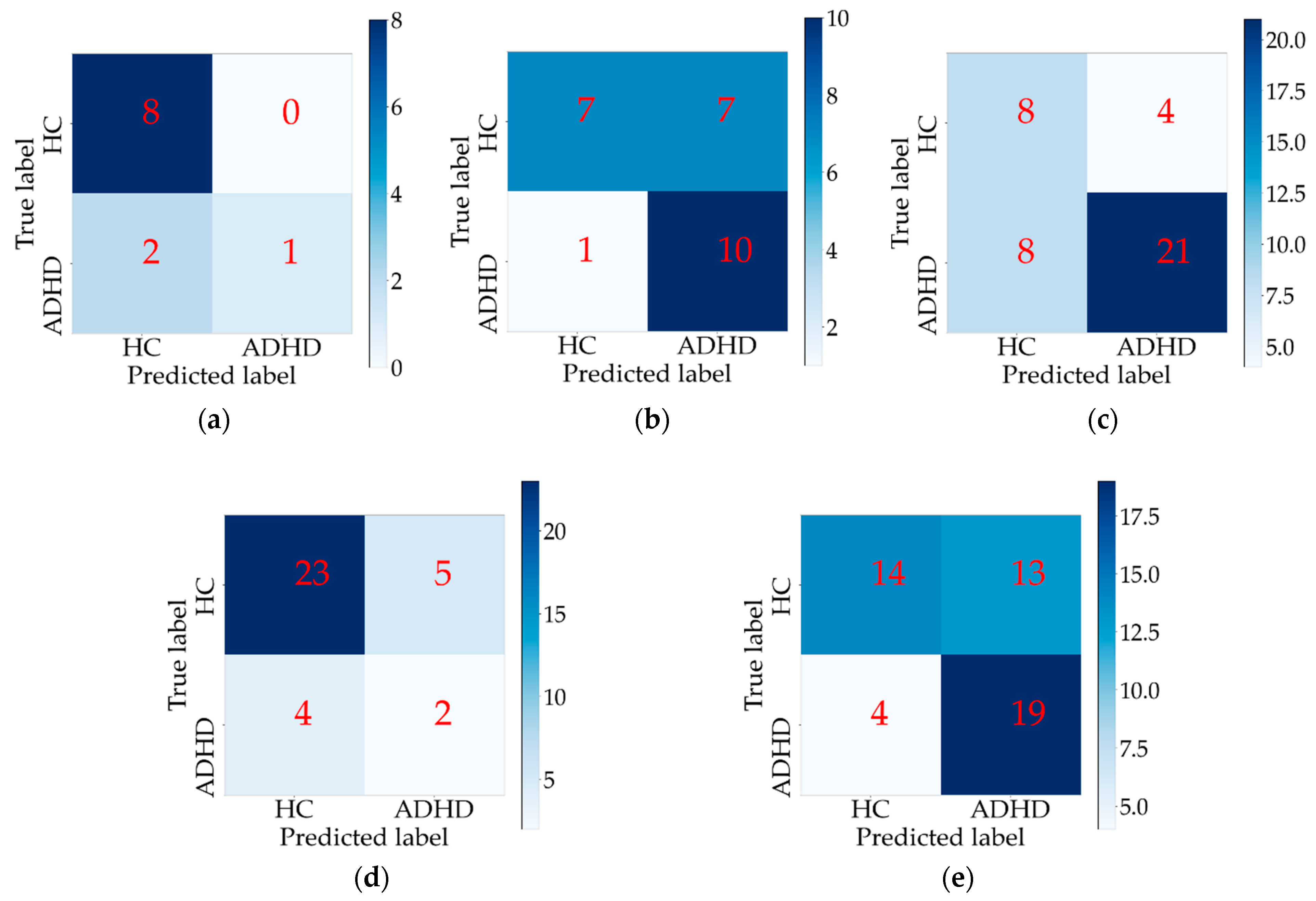
. The fMRI data had the dual characteristics of imbalance and high dimension. In the high-dimensional feature space, the data distribution was sparser and contained more redundant and irrelevant features. It was usually difficult to obtain effective information from the preprocessed fMRI data, which made it more difficult to identify ADHD. Therefore, the sensitivity of all the methods in Table 3 was generally not high. Compared with the other three methods, our proposed method achieved better performances on all five test sets, which means that our method has better generalization ability when applied to different data sets. Especially, the classification accuracy and sensitivity on NYU were significantly better in our method than in the other methods. The confusion matrices of the classification results in the individual site experiments are shown in Figure 4. It can be observed from Figure 4c that most samples of HC and ADHD in the NYU data set could be classified correctly, the reason for which was perhaps because the samples of ADHD in NYU were more than that of HC.

4.3. Classification Experiment of Training on Combining Site Data and Test on Benchmark Test Data

The ADHD classification experiment of training on combining site data and test on benchmark test data, combining site experiment for short, refers to combining the training data of all five imaging sites in Table 1 as the training set to train the model and then taking the benchmark test data set of each imaging site used in the competition of ADHD-200 as the test set for the classification experiment. For example, in the NYU classification of the combining site experiment, there were 619 training samples, which were obtained by combining the training data of these five imaging sites (i.e., KKI, NI, NYU, OHSU, and Peking) shown in Table 1, and there were 41 test samples, which were the benchmark test set of the NYU imaging site. In the combining site experiment, the weight of the cross-loss function α was set to 2. The ADHD classification results on the combining site experiment of different methods are displayed in

Table 4. Classification accuracies (%) comparison of the different methods in the combining site experiment.

Method	KKI	NI	NYU	OHSU	Peking	Average
ADHD-200 (2012) [23]	61.9	56.95	35.19	65.37	51.05	54.09
Fusion of fMRI and non-imaging data (2018) [7]	81.8	-	56.1	-	60.7	66.2
DeepFMRI (2020) [15]	-	60	65.8	-	43.1	56.3
SC-CNN-Attention (2020) [16]	77.7	75.3	60.4	64.4	65.2	68.6
Our proposed method	81.82	68	70.73	73.53	66	72.02

, which shows that the proposed method performed well in general compared to the most advanced methods, especially in the case of the OHSU data set, where the recognition accuracy was much higher than the other methods and also achieved an average accuracy of 72.02%, a state-of-the-art performance.

The specificity, sensitivity, and accuracy of the proposed method in the combining site experiment are shown in

Table 5. The specificity (%), sensitivity (%), and accuracy (%) of our proposed method in the combining site experiment.

Evaluation Metrics	KKI	NI	NYU	OHSU	Peking
Specificity	100	50	66.67	82.14	51.85
Sensitivity	33.33	90.91	72.41	33.33	82.61
Accuracy	81.82	68	70.73	73.53	66

. Increasing the training samples, the sensitivities of NI and Peking were significantly improved compared to the individual site experiments. At the same time, it can also be observed that the imbalance of the test sets in KKI and OHSU was severe, and the number of ADHD samples in these test sets was small, which resulted in the low sensitivity of KKI and OHSU in the combining site experiment. The confusion matrices of the classification results in the combining site experiment are shown in Figure 5.

4.4. Comparative Experiment of Pre-trained Network Freezing and Pre-trained Network Fine-tuning

As the pre-trained network was trained on a large data set, it was usually used to keep the network structure unchanged but with fine-tuned weight by transferring the knowledge to another scene effectively. Considering the small number of samples in the individual site experiment, the mode by freezing all the pre-trained neural network parameters was adopted to reduce the number of updatable parameters in this paper. Freezing is an effective way to avoid the probable overfitting when only a few training samples are available in the deep neural network. Relatively speaking, there are a few more samples in the combining site experiment, so the method of fine-tuning the pre-trained neural network parameters was adopted in the combining site experiment.

The statistics of the trainable and untrainable parameters in the representation learning neural network are shown in

Table 6. Parameter number statistics of the representation learning neural network in the freezing mode and fine-tuning mode.

Statistical Item	Representation Learning Neural Network	Freezing	Fine-Tuning
Sub module	Channel sequence representation learning module	220	220
	Pre-trained neural network (ResNet34)	21,284,672	21,284,672
	MLP classifier	1025	1025
Trainable/untrained	Trainable parameters	1245	21,285,917
	Untrainable parameters	21,284,672	0
Total number of parameters		21,285,917	21,285,917

, where the pre-trained network was ResNet34 and the time-series length s was set to 73. Obviously, the number of parameters for each submodule in the freezing mode and that in the fine-tuning mode were equal. It can be seen from Table 6 that the number of untrainable parameters in the pre-trained neural network in the fine-tuning mode was zero, which means all parameters would be updated in the network training process. For the freezing mode, the number of trainable parameters was 1245, where its value was the sum of 220 parameters of the channel sequence representation learning module and 1025 parameters of the MLP classifier. Because the channel sequence representation learning module was realized by a 1 × 1 × s convolution operation, and the number of convolution kernels was 3, when s = 73, the number of the convolution layer parameter was 73 × 3 plus a bias; that is, the number of parameters of the channel sequence representation learning module was 220. Through a full connection layer, the 512-dimensional representation vector f extracted by the pre-trained network ResNet34 was mapped to a vector y with a length of 2, so the number of parameters for the MLP classifier was 1025.

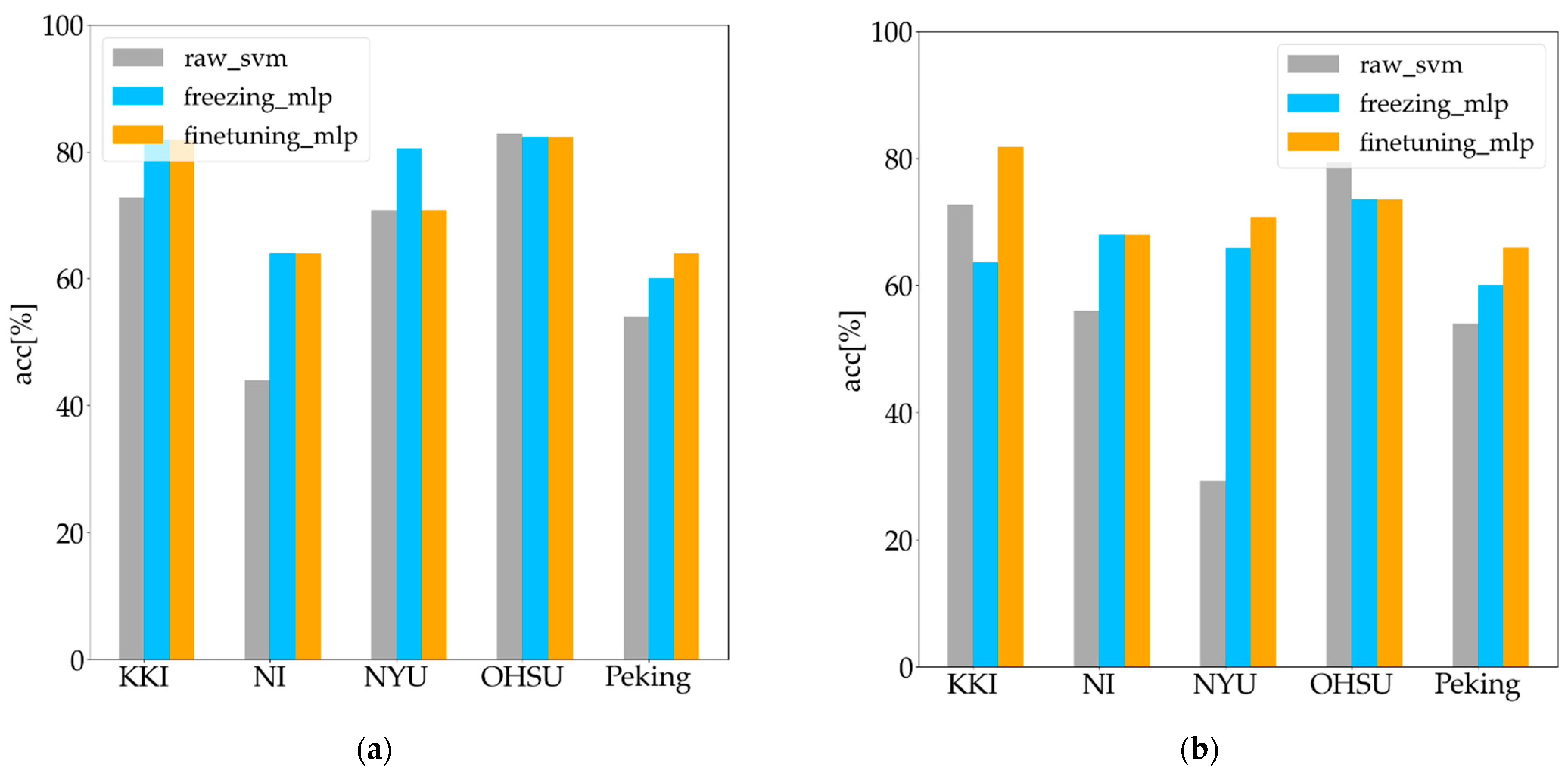
To verify the effectiveness of the sequence representation learning network proposed in this paper, the ADHD classification experiments of the pre-trained network freezing and pre-trained network fine-tuning are carried out in this section. The pre-trained network ResNet34 and the MLP classifier were used. These two methods were recorded as freezing_mlp and finetuning_mlp, respectively. At the same time, the SVM classification experiment directly using the preprocessed fMRI sequence data X_TS as input was performed, and the method was recorded as raw_svm. The comparison of the ADHD classification experimental results of the above three methods is shown in Figure 6.

As can be seen from Figure 6, in the individual site experiment, little difference exists between the freezing mode and fine-tuning mode in the classification accuracy for the five sites. The average classification accuracies of freezing_mlp, finetuning_mlp, and raw_svm were 73.73%, 72.58%, and 64.76%, respectively. In the combining site experiment, the classification accuracy of the fine-tuning mode was generally higher than that of the freezing mode for all sites, where the average classification accuracies of freeze_mlp, fine-tune_mlp, and raw_svm were 66.2%, 72.02%, and 58.28%, respectively.

4.5. Comparative Experiment of Weight Setting in Cross-Entropy Loss Function

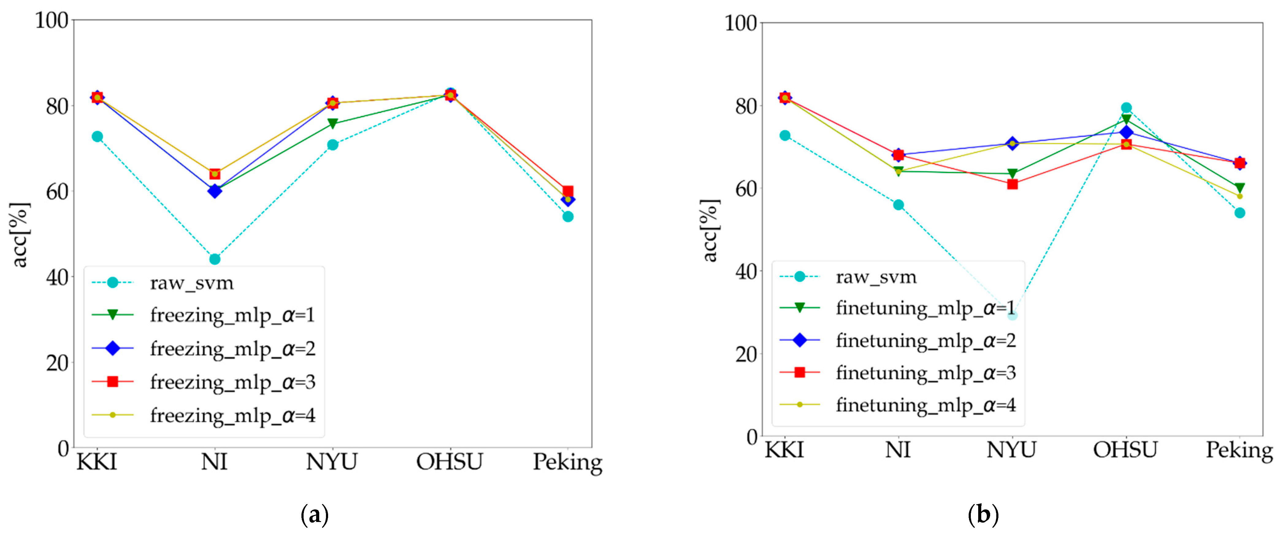
As explained in Section 3.4.3, to alleviate the problem of sample imbalance, this method uses weighted cross-entropy as a loss function. In both the individual site experiments and the combining site experiment, the classification results with different weights are shown in Figure 7. As described in Section 4.4 above, because the freezing mode in the individual site experiment was slightly better than the fine-tuning mode, only the classification results of the freezing mode were listed in the individual site experiments, and the classification accuracies with different α values are shown in Figure 7a. Similarly, the fine-tuning mode in the combining site experiment was slightly better than the freezing mode, so only the classification results of the fine-tuning mode were listed in the combining site experiment, and the classification accuracies with different α values are shown in Figure 7b. Figure 7a,b show that the overall classification accuracy improved with the increasing weight α of the ADHD samples in the cross-entropy loss function on the condition that α > 1. Although the data imbalance at the different imaging sites was different, the overall performance of the classification in the individual site experiments was optimal for each test data when α was equal to three. On the other hand, compared to α = 1, α = 4, and raw_svm, the classification accuracy in the combining site experiment remained the highest in most sites (three of five) with the same setting, α = 3. However, setting α = 2 seemed to be optimal for the overall performance of classification in the combining site experiment.

4.6. Computational Complexity

The computational power needs to be considered when running the deep learning algorithm. The computational complexity of the deep learning algorithm is generally measured by the number of floating-point operations (FLOPs).

In our proposed method, firstly, the two-dimensional time sequence matrix, X_TS, was transformed into a three-dimensional image, X_IMG, by the data conversion module, and then the sequence feature learning neural network was conducted for representation learning and classification. Because the data conversion module performed the conversion from X_TS to X_IMG by a reshaping function quickly and this module did not involve parameter learning, the cost time of the data conversion module was ignored. Therefore, the FLOPs of the proposed method refer to the FLOPs of the sequence representation learning neural network. In this paper, the ptflops [24], a FLOPs counter for convolutional networks in the PyTorch framework, was used to calculate the computational complexity of the neural networks.

Table 7. The FLOPs of our proposed method.

Submodule	Output Shape	Computational Complexity of the Submodule	Total Computational Complexity
Data conversion	(54, 54, 73)	0	267.697 MFLOPs
Channel sequence representation learning module	(54, 54, 3)	0.639 MFLOPs
Pre-trained neural network (ResNet34)	(512)	267.057 MFLOPs
MLP classifier	(2)	0.001 MFLOPs

shows the FLOPs of our proposed method.

5. Discussion

In this paper, we proposed an fMRI sequence representation learning framework and demonstrated its application to ADHD classification. The sequence representation learning framework was mainly composed of an fMRI data preprocessing module, a data conversion module, and a sequence representation learning neural network. The data conversion module transformed the two-dimensional sequence, X_TS, into the three-dimensional image, X_IMG, the rationale for which can be described from three aspects. First, if a 3 × 3 convolution kernel is used for the convolution operation on the three-dimensional image, X_IMG, the relationships among the nine adjacent regions of interest can be modeled, and the modeling area becomes larger than that of the convolution operation on the two-dimensional sequence, X_TS. Second, the channel sequence representation learning module can easily and effectively capture the discriminative low-level channel-wise features of the fMRI data by the operating convolution with a 1 × 1 × s kernel on the X_IMG. Three, after the operation of the data conversion and the channel sequence representation learning, the image size was much smaller than X_TS. Therefore, the computational complexity of the convolution operation on the pre-trained neural network was greatly reduced.

Aimed at the problem of a few ADHD samples, the transfer learning method was used to freeze or fine-tune the pre-trained neural network parameters to reduce the risk of overfitting. We have leveraged a transfer learning strategy where a deep network model such as ResNet is pre-trained using a large-scale natural image dataset, such as the ImageNet dataset [25], given the fact that different types of images share common features. This strategy has been successful in many applications, including those for medical data, for example, the detection of erythema migrans [26]. Further, there are two main reasons why our proposed framework with the pre-trained ResNet model trained on the ImageNet dataset can achieve satisfactory classification performances. One of the reasons may be that the ImageNet dataset is massive. The model trained from large-scale data sets has better representation ability. Generally, the layers of the neural network are deeper, and the representation ability of the model is higher. Another reason may be that the ResNet with deep layers can capture discriminative features for ADHD classification. To explore the effectiveness of the sequence representation learning network based on transfer learning, we carried out experiments using the pre-trained network freezing method and pre-trained network fine-tuning method and compared them with the raw_svm method. As can be seen from Figure 6, in general, both in the individual site experiment and the combining site experiment, the classification accuracies of the freezing_mlp and finetuning_mlp proposed in this paper were higher than that of the raw_svm method.

To alleviate the problem of sample imbalance, the proposed method used weighted cross-entropy as a loss function. To explore the influence of weight α in the cross-entropy loss function on the classification performance, the individual site experiment and the combining site experiment with different α values were conducted. The results are presented in Figure 7a,b, which show that with the increase in weight α of the ADHD samples in the cross-entropy loss function, for instance, when setting α > 1, the overall classification accuracy can be improved. Generally speaking, the classification accuracy increases with the increase in the number of training samples. However, due to the heterogeneity of the fMRI data induced by the differences in the image acquisitions across the different sites, such as MRI scanners and pulse sequences, compared with the individual site experiment, the classification accuracy of the combining site experiment did not always improve with the increase in the number of training samples, and the classification accuracies appeared to fluctuate with different α values. Despite these challenges induced by the imbalance of samples and data heterogeneity, our method can achieve a robust classification performance in the individual site experiments and the combining site experiment.

The experimental results showed that in the case of a few training samples and sample imbalance, the proposed method is efficient and feasible, which can effectively extract the discriminative representations of a brain region time series. It is worth noticing that the proposed method did not use the traditional data augmentation for deep learning and complex representation selection technology to improve the effect.

Due to the lack of interpretability of the deep neural network, it was still unable to reveal the corresponding pathological neurobiological mechanism from the hidden representation in a deep neural network, which will also be an important research direction of deep learning applied to medical image processing in the future.

6. Conclusions

To tackle the issues that DL needs large samples, and the medical samples of ADHD are small and imbalanced, an fMRI sequence representation learning framework was proposed and applied to ADHD classification. The ADHD-200 classification average accuracies of the proposed method for individual imaging site experiments and the combining imaging site experiment were 73.73% and 72.02%, representing state-of-the-art performance. The experimental results showed that our proposed method could effectively extract the discriminative representations for ADHD classification. The proposed method is simple and effective, which can be easily extended to the diagnosis of other brain nerve diseases.