
Exploring the Utility of Anonymized EHR Datasets in Machine Learning Experiments in the Context of the MODELHealth Project

 ,
,  , , and
Abstract
:1. Introduction
2. Materials and Methods
2.1. Data
2.2. Anonymization and Information Loss Estimation
2.2.1. K-Anonymity
2.2.2. L-Diversity, T-Closeness
2.2.3. Mondrian Algorithm
2.2.4. Information Loss
2.3. Machine Learning
2.3.1. Logistic Regression
2.3.2. Decision Trees
2.3.3. K Nearest Neighbors
2.3.4. Support Vector Machines
2.3.5. Gaussian Naive Bayes
3. Results
4. Discussion
5. Conclusions
Author Contributions
Funding
Informed Consent Statement
Data Availability Statement
Conflicts of Interest
Appendix A

| Machine Learning Model | Parameters |
|---|---|
| Logistic Regression | C = 1.0, class_weight = None, dual = False, fit_intercept = True, intercept_scaling = 1, l1_ratio = None, max_iter = 100, multi_class = ‘auto’, n_jobs = None, penalty = ‘l2′, random_state = None, solver = ‘liblinear’, tol = 0.0001, verbose = 0, warm_start = False |
| Decision Tree Classifier | ccp_alpha = 0.0, class_weight = None, criterion = ‘gini’, max_depth = None, max_features = None, max_leaf_nodes = None, min_impurity_decrease = 0.0, min_impurity_split = None, min_samples_leaf = 1, min_samples_split = 2, min_weight_fraction_leaf = 0.0, presort = ‘deprecated’, random_state = None, splitter = ‘best’ |
| KNeighborsClassifier | algorithm = ‘auto’, leaf_size = 30, metric = ‘minkowski’, metric_params = None, n_jobs = None, n_neighbors = 5, p = 2, weights = ‘uniform’ |
| GaussianNB | priors = None, var_smoothing = 1 × 10⁻⁹ |
| SVC | C = 1.0, break_ties = False, cache_size = 200, class_weight = None, coef0 = 0.0, decision_function_shape = ‘ovr’, degree = 3, gamma = ‘auto’, kernel = ‘rbf’, max_iter = −1, probability = False, random_state = None, shrinking = True, tol = 0.001, verbose = False |
| Classifier | QI | k | GIL | DM | CAVG | Train AUC | Validation AUC | Test AUC | Test MCC |
|---|---|---|---|---|---|---|---|---|---|
| Logistic Regression | 0 | 1 | 0 | 0 | 0 | 0.723 | 0.723 | 0.723 | 0.456 |
| 2 | 2 | 0.394 | 346,873,092 | 492.353 | 0.736 | 0.729 | 0.735 | 0.477 | |
| 3 | 0.394 | 346,873,108 | 331.017 | 0.717 | 0.709 | 0.716 | 0.438 | ||
| 5 | 0.394 | 346,873,168 | 202.034 | 0.725 | 0.716 | 0.724 | 0.454 | ||
| 10 | 0.394 | 346,873,396 | 102.789 | 0.726 | 0.719 | 0.725 | 0.457 | ||
| 15 | 0.394 | 346,875,014 | 70.378 | 0.73 | 0.723 | 0.729 | 0.465 | ||
| 20 | 0.394 | 346,878,574 | 54.25 | 0.724 | 0.719 | 0.723 | 0.454 | ||
| 30 | 0.394 | 346,884,568 | 37.558 | 0.719 | 0.717 | 0.719 | 0.445 | ||
| 3a | 2 | 0.352 | 254,366,790 | 209.25 | 0.685 | 0.661 | 0.682 | 0.365 | |
| 3 | 0.352 | 254,366,928 | 144.133 | 0.701 | 0.685 | 0.7 | 0.401 | ||
| 5 | 0.352 | 254,367,482 | 91.547 | 0.692 | 0.674 | 0.69 | 0.38 | ||
| 10 | 0.353 | 254,371,334 | 50.509 | 0.689 | 0.668 | 0.687 | 0.374 | ||
| 15 | 0.353 | 254,378,570 | 36 | 0.679 | 0.649 | 0.676 | 0.352 | ||
| 20 | 0.354 | 254,353,268 | 28.721 | 0.69 | 0.672 | 0.688 | 0.377 | ||
| 30 | 0.355 | 254,372,510 | 20.134 | 0.686 | 0.667 | 0.684 | 0.369 | ||
| 3b | 2 | 0.214 | 75,443,862 | 21.275 | 0.747 | 0.732 | 0.746 | 0.493 | |
| 3 | 0.215 | 75,448,478 | 16.502 | 0.748 | 0.719 | 0.745 | 0.493 | ||
| 5 | 0.216 | 75,461,502 | 11,83 | 0.753 | 0.729 | 0.75 | 0.502 | ||
| 10 | 0.219 | 75,530,606 | 7.73 | 0.75 | 0.727 | 0.748 | 0.497 | ||
| 15 | 0.22 | 75,632,804 | 6.005 | 0.752 | 0.721 | 0.749 | 0.499 | ||
| 20 | 0.222 | 75,820,294 | 5.208 | 0.736 | 0.708 | 0.733 | 0.467 | ||
| 30 | 0.225 | 76,159,906 | 4.099 | 0.745 | 0.718 | 0.742 | 0.487 | ||
| 4 | 2 | 0.085 | 7,964,110 | 3.789 | 0.778 | 0.733 | 0.773 | 0.548 | |
| 3 | 0.093 | 8,016,196 | 3.434 | 0.779 | 0.726 | 0.774 | 0.549 | ||
| 5 | 0.104 | 8,145,452 | 3.012 | 0.782 | 0.731 | 0.777 | 0.554 | ||
| 10 | 0.116 | 8,563,030 | 2.525 | 0.778 | 0.725 | 0.773 | 0.546 | ||
| 15 | 0.123 | 9,082,286 | 2.304 | 0.776 | 0.717 | 0.77 | 0.541 | ||
| 20 | 0.126 | 9,621,138 | 2.138 | 0.767 | 0.713 | 0.762 | 0.525 | ||
| 30 | 0.131 | 10,880,770 | 1.953 | 0.766 | 0.721 | 0.761 | 0.522 | ||
| Decision Tree Classifier | 0 | 1 | 0 | 0 | 0 | 0.959 | 0.658 | 0.929 | 0.861 |
| 2 | 2 | 0.394 | 346,873,092 | 492.353 | 0.941 | 0.67 | 0.914 | 0.83 | |
| 3 | 0.394 | 346,873,108 | 331.017 | 0.934 | 0.655 | 0.906 | 0.814 | ||
| 5 | 0.394 | 346,873,168 | 202.034 | 0.938 | 0.657 | 0.91 | 0.821 | ||
| 10 | 0.394 | 346,873,396 | 102.789 | 0.936 | 0.663 | 0.908 | 0.818 | ||
| 15 | 0.394 | 346,875,014 | 70.378 | 0.94 | 0.657 | 0.911 | 0.824 | ||
| 20 | 0.394 | 346,878,574 | 54.25 | 0.941 | 0.669 | 0.914 | 0.83 | ||
| 30 | 0.394 | 346,884,568 | 37.558 | 0.94 | 0.66 | 0.912 | 0.825 | ||
| 3a | 2 | 0.352 | 254,366,790 | 209.25 | 0.916 | 0.65 | 0.889 | 0.781 | |
| 3 | 0.352 | 254,366,928 | 144.133 | 0.921 | 0.654 | 0.894 | 0.792 | ||
| 5 | 0.352 | 254,367,482 | 91.547 | 0.917 | 0.654 | 0.891 | 0.784 | ||
| 10 | 0.353 | 254,371,334 | 50509 | 0.918 | 0.649 | 0.892 | 0.785 | ||
| 15 | 0.353 | 254,378,570 | 36 | 0.91 | 0.636 | 0.882 | 0.766 | ||
| 20 | 0.354 | 254,353,268 | 28.721 | 0.911 | 0.64 | 0.884 | 0.774 | ||
| 30 | 0.355 | 254,372,510 | 20.134 | 0.92 | 0.657 | 0.894 | 0.791 | ||
| 3b | 2 | 0.214 | 75,443,862 | 21.275 | 0.933 | 0.662 | 0.906 | 0.813 | |
| 3 | 0.215 | 75,448,478 | 16.502 | 0.936 | 0.666 | 0.909 | 0.821 | ||
| 5 | 0.216 | 75,461,502 | 11.83 | 0.937 | 0.667 | 0.91 | 0.821 | ||
| 10 | 0.219 | 75,530,606 | 7.73 | 0.939 | 0.687 | 0.914 | 0.829 | ||
| 15 | 0.22 | 75,632,804 | 6.005 | 0.939 | 0.674 | 0.912 | 0.826 | ||
| 20 | 0.222 | 75,820,294 | 5.208 | 0.93 | 0.646 | 0.902 | 0.806 | ||
| 30 | 0.225 | 76,159,906 | 4.099 | 0.933 | 0.675 | 0.907 | 0.817 | ||
| 4 | 2 | 0.085 | 7,964,110 | 3.789 | 0.946 | 0.664 | 0.918 | 0.837 | |
| 3 | 0.093 | 8,016,196 | 3.434 | 0.941 | 0.679 | 0.915 | 0.835 | ||
| 5 | 0.104 | 8,145,452 | 3.012 | 0.943 | 0.686 | 0.918 | 0.837 | ||
| 10 | 0.116 | 8,563,030 | 2.525 | 0.94 | 0.671 | 0.913 | 0.827 | ||
| 15 | 0.123 | 9,082,286 | 2.304 | 0.941 | 0.671 | 0.914 | 0.83 | ||
| 20 | 0.126 | 9,621,138 | 2.138 | 0.933 | 0.67 | 0.907 | 0.819 | ||
| 30 | 0.131 | 10,880,770 | 1.953 | 0.932 | 0.676 | 0.906 | 0.814 | ||
| KNN | 0 | 1 | 0 | 0 | 0 | 0.793 | 0.712 | 0.785 | 0.57 |
| 2 | 2 | 0.394 | 346,873,092 | 492.353 | 0.784 | 0.702 | 0.776 | 0.553 | |
| 3 | 0.394 | 346,873,108 | 331.017 | 0.772 | 0.686 | 0.763 | 0.527 | ||
| 5 | 0.394 | 346,873,168 | 202.034 | 0.782 | 0.691 | 0.773 | 0.546 | ||
| 10 | 0.394 | 346,873,396 | 102.789 | 0.778 | 0.702 | 0.771 | 0.542 | ||
| 15 | 0.394 | 346,875,014 | 70.378 | 0.778 | 0.702 | 0.771 | 0.542 | ||
| 30 | 0.394 | 346,884,568 | 37.558 | 0.779 | 0.694 | 0.771 | 0.542 | ||
| 20 | 0.394 | 346,878,574 | 54.25 | 0.772 | 0.683 | 0.763 | 0.527 | ||
| 3a | 2 | 0.352 | 254,366,790 | 209.25 | 0.764 | 0.671 | 0.755 | 0.51 | |
| 3 | 0.352 | 254,366,928 | 144.133 | 0.775 | 0.691 | 0.767 | 0.534 | ||
| 5 | 0.352 | 254,367,482 | 91.547 | 0.763 | 0.673 | 0.754 | 0.508 | ||
| 10 | 0.353 | 254,371,334 | 50.509 | 0.764 | 0.671 | 0.755 | 0.51 | ||
| 15 | 0.353 | 254,378,570 | 36 | 0.758 | 0.664 | 0.749 | 0.497 | ||
| 20 | 0.354 | 254,353,268 | 28.721 | 0.756 | 0.661 | 0.746 | 0.493 | ||
| 30 | 0.355 | 254,372,510 | 20.134 | 0.761 | 0.668 | 0.752 | 0.505 | ||
| 3b | 2 | 0.214 | 75,443,862 | 21.275 | 0.783 | 0.704 | 0.775 | 0.551 | |
| 3 | 0.215 | 75,448,478 | 16.502 | 0.788 | 0.712 | 0.78 | 0.563 | ||
| 5 | 0.216 | 75,461,502 | 11.83 | 0.771 | 0.691 | 0.763 | 0.526 | ||
| 10 | 0.219 | 75,530,606 | 7.73 | 0.789 | 0.708 | 0.781 | 0.562 | ||
| 15 | 0.22 | 75,632,804 | 6.005 | 0.778 | 0.693 | 0.77 | 0.541 | ||
| 20 | 0.222 | 75,820,294 | 5.208 | 0.771 | 0.68 | 0.762 | 0.525 | ||
| 30 | 0.225 | 76,159,906 | 4.099 | 0.781 | 0.695 | 0.772 | 0.545 | ||
| 4 | 2 | 0.085 | 7,964,110 | 3.789 | 0.782 | 0.693 | 0.773 | 0.547 | |
| 3 | 0.093 | 8,016,196 | 3.434 | 0.785 | 0.694 | 0.776 | 0.552 | ||
| 5 | 0.104 | 8,145,452 | 3.012 | 0.788 | 0.71 | 0.78 | 0.561 | ||
| 10 | 0.116 | 8,563,030 | 2.525 | 0.78 | 0.702 | 0.773 | 0.545 | ||
| 15 | 0.123 | 9,082,286 | 2.304 | 0.792 | 0.7 | 0.783 | 0.566 | ||
| 20 | 0.126 | 9,621,138 | 2.138 | 0.785 | 0.702 | 0.777 | 0.553 | ||
| 30 | 0.131 | 10,880,770 | 1.953 | 0.776 | 0.696 | 0.768 | 0.537 | ||
| Gaussian NB | 0 | 1 | 0 | 0 | 0 | 0.708 | 0.708 | 0.708 | 0.431 |
| 2 | 2 | 0.394 | 346,873,092 | 492.353 | 0.561 | 0.55 | 0.56 | 0.184 | |
| 3 | 0.394 | 346,873,108 | 331.017 | 0.558 | 0.548 | 0.557 | 0.196 | ||
| 5 | 0.394 | 346,873,168 | 202.034 | 0.554 | 0.547 | 0.553 | 0.192 | ||
| 10 | 0.394 | 346,873,396 | 102.789 | 0.539 | 0.529 | 0.538 | 0.154 | ||
| 15 | 0.394 | 346,875,014 | 70.378 | 0.56 | 0.543 | 0.559 | 0.179 | ||
| 20 | 0.394 | 346,878,574 | 54.25 | 0.57 | 0.55 | 0.568 | 0.191 | ||
| 30 | 0.394 | 346,884,568 | 37.558 | 0.56 | 0.549 | 0.559 | 0.193 | ||
| 3a | 2 | 0.352 | 254,366,790 | 209.25 | 0.559 | 0.548 | 0.558 | 0.212 | |
| 3 | 0.352 | 254,366,928 | 144.133 | 0.554 | 0.543 | 0.553 | 0.192 | ||
| 5 | 0.352 | 254,367,482 | 91.547 | 0.563 | 0.551 | 0.561 | 0.209 | ||
| 10 | 0.353 | 254,371,334 | 50.509 | 0.554 | 0.538 | 0.553 | 0.182 | ||
| 15 | 0.353 | 254,378,570 | 36 | 0.563 | 0.549 | 0.561 | 0.209 | ||
| 20 | 0.354 | 254,353,268 | 28.721 | 0.561 | 0.551 | 0.56 | 0.205 | ||
| 30 | 0.355 | 254,372,510 | 20.134 | 0.553 | 0.539 | 0.551 | 0.186 | ||
| 3b | 2 | 0.214 | 75,443,862 | 21.275 | 0.568 | 0.544 | 0.566 | 0.218 | |
| 3 | 0.215 | 75,448,478 | 16.502 | 0.577 | 0.554 | 0.575 | 0.24 | ||
| 5 | 0.216 | 75,461,502 | 11.83 | 0.56 | 0.534 | 0.557 | 0.206 | ||
| 10 | 0.219 | 75,530,606 | 7.73 | 0.577 | 0.55 | 0.574 | 0.246 | ||
| 15 | 0.22 | 75,632,804 | 6.005 | 0.586 | 0.55 | 0.582 | 0.237 | ||
| 20 | 0.222 | 75,820,294 | 5.208 | 0.568 | 0.539 | 0.565 | 0.218 | ||
| 30 | 0.225 | 76,159,906 | 4.099 | 0.568 | 0.544 | 0.566 | 0.22 | ||
| 4 | 2 | 0.085 | 7,964,110 | 3.789 | 0.618 | 0.55 | 0.611 | 0.347 | |
| 3 | 0.093 | 8,016,196 | 3.434 | 0.626 | 0.544 | 0.618 | 0.363 | ||
| 5 | 0.104 | 8,145,452 | 3.012 | 0.641 | 0.558 | 0.633 | 0.383 | ||
| 10 | 0.116 | 8,563,030 | 2.525 | 0.627 | 0.555 | 0.62 | 0.355 | ||
| 15 | 0.123 | 9,082,286 | 2.304 | 0.638 | 0.572 | 0.632 | 0.379 | ||
| 20 | 0.126 | 9,621,138 | 2.138 | 0.652 | 0.581 | 0.645 | 0.388 | ||
| 30 | 0.131 | 10,880,770 | 1.953 | 0.661 | 0.61 | 0.656 | 0.397 | ||
| SVC | 0 | 1 | 0 | 0 | 0 | 0.711 | 0.711 | 0.711 | 0.437 |
| 2 | 2 | 0.394 | 346,873,092 | 492.353 | 0.709 | 0.709 | 0.709 | 0.431 | |
| 3 | 0.394 | 346,873,108 | 331.017 | 0.686 | 0.686 | 0.686 | 0.387 | ||
| 5 | 0.394 | 346,873,168 | 202.034 | 0.688 | 0.688 | 0.688 | 0.391 | ||
| 10 | 0.394 | 346,873,396 | 102.789 | 0.695 | 0.695 | 0.695 | 0.404 | ||
| 15 | 0.394 | 346,875,014 | 70.378 | 0.703 | 0.703 | 0.703 | 0.421 | ||
| 20 | 0.394 | 346,878,574 | 54.25 | 0.701 | 0.7 | 0.701 | 0.416 | ||
| 30 | 0.394 | 346,884,568 | 37.558 | 0.69 | 0.691 | 0.69 | 0.397 | ||
| 3a | 2 | 0.352 | 254,366,790 | 209.25 | 0.571 | 0.571 | 0.571 | 0.221 | |
| 3 | 0.352 | 254,366,928 | 144.133 | 0.584 | 0.57 | 0.583 | 0.222 | ||
| 5 | 0.352 | 254,367,482 | 91.547 | 0.588 | 0.578 | 0.587 | 0.22 | ||
| 10 | 0.353 | 254,371,334 | 50.509 | 0.583 | 0.581 | 0.583 | 0.217 | ||
| 15 | 0.353 | 254,378,570 | 36 | 0.568 | 0.567 | 0.568 | 0.21 | ||
| 20 | 0.354 | 254,353,268 | 28.721 | 0.593 | 0.59 | 0.592 | 0.213 | ||
| 30 | 0.355 | 254,372,510 | 20.134 | 0.579 | 0.578 | 0.579 | 0.176 | ||
| 3b | 2 | 0.214 | 75,443,862 | 21.275 | 0.695 | 0.695 | 0.695 | 0.402 | |
| 3 | 0.215 | 75,448,478 | 16.502 | 0.7 | 0.7 | 0.7 | 0.416 | ||
| 5 | 0.216 | 75,461,502 | 11.83 | 0.696 | 0.696 | 0.696 | 0.407 | ||
| 10 | 0.219 | 75,530,606 | 7.73 | 0.694 | 0.694 | 0.694 | 0.405 | ||
| 15 | 0.22 | 75,632,804 | 6.005 | 0.703 | 0.703 | 0.703 | 0.422 | ||
| 20 | 0.222 | 75,820,294 | 5.208 | 0.681 | 0.681 | 0.681 | 0.379 | ||
| 30 | 0.225 | 76,159,906 | 4.099 | 0.698 | 0.697 | 0.698 | 0.409 | ||
| 4 | 2 | 0.085 | 7,964,110 | 3.789 | 0.72 | 0.721 | 0.72 | 0.444 | |
| 3 | 0.093 | 8,016,196 | 3.434 | 0.714 | 0.712 | 0.714 | 0.433 | ||
| 5 | 0.104 | 8,145,452 | 3.012 | 0.707 | 0.704 | 0.707 | 0.423 | ||
| 10 | 0.116 | 8,563,030 | 2.525 | 0.703 | 0.699 | 0.702 | 0.416 | ||
| 15 | 0.123 | 9,082,286 | 2.304 | 0.696 | 0.696 | 0.696 | 0.407 | ||
| 20 | 0.126 | 9,621,138 | 2.138 | 0.69 | 0.689 | 0.69 | 0.396 | ||
| 30 | 0.131 | 10,880,770 | 1.953 | 0.696 | 0.695 | 0.695 | 0.405 |
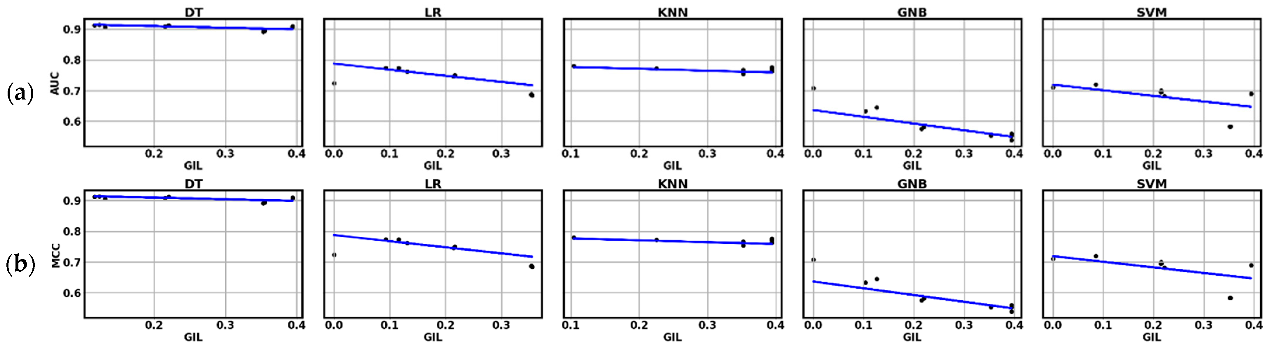
| Machine Learning Model | Linear Regression AUC vs. GIL | Linear Regression MCC vs. GIL |
|---|---|---|
| Logistic Regression | yAUC = 0.77886 − 0.1914 × xGIL | yMCC = 0.54762 − 0.3393 × xGIL |
| Decision Tree Classifier | yAUC = 0.9182 − 0.03648 × xGIL | yMCC = 0.84385 − 0.1185 × xGIL |
| KNeighborsClassifier | yAUC = 0.78136 − 0.04867 × xGIL | yMCC = 0.56195 − 0.0921 × xGIL |
| GaussianNB | yAUC = 0.659 − 0.2924 × xGIL | yMCC = 0.41258 − 0.6357 × xGIL |
| SVC | yAUC = 0.72082 − 0.1865 × xGIL | yMCC = 0.44355 − 0.26539528 × xGIL |
| f | df1 | df2 | p | |
|---|---|---|---|---|
| Test MCC | 908 | 4 | 65.9 | <0.001 |
| Test AUC | 1163 | 4 | 65.6 | <0.001 |
| DecisionTreeClassifier | GaussianNB | KNN | LogisticRegression | SVC | ||
|---|---|---|---|---|---|---|
| Decision Tree classifier | Mean difference | - | 0.563 *** | 0.277 *** | 0.3497 *** | 0.452 *** |
| p-value | - | <0.001 | <0.001 | <0.001 | <0.001 | |
| Gaussian NB | Mean difference | - | −0.285 *** | −0.2129 *** | −0.111 *** | |
| p-value | - | <0.001 | <0.001 | <0.001 | ||
| KNN | Mean difference | - | 0.0723 *** | 0.174 *** | ||
| p-value | - | <0.0001 | <0.001 | |||
| Logistic Regression | Mean difference | - | 0.102 *** | |||
| p-value | - | <0.001 | ||||
| SVC | Mean difference | - | ||||
| p-value | - |
| DecisionTreeClassifier | GaussianNB | KNN | LogisticRegression | SVC | ||
|---|---|---|---|---|---|---|
| Decision Tree classifier | Mean difference | - | 0.348 *** | 0.156 *** | 0.1995 *** | 0.2629 *** |
| p-value | - | <0.001 | <0.001 | <0.001 | <0.001 | |
| Gaussian NB | Mean difference | - | −0.191 *** | −0.1481 *** | −0.0848 *** | |
| p-value | - | <0.001 | <0.001 | <0.001 | ||
| KNN | Mean difference | - | 0.0431 *** | 0.1065 *** | ||
| p-value | - | <0.0001 | <0.001 | |||
| Logistic Regression | Mean difference | - | 0.0633 *** | |||
| p-value | - | <0.001 | ||||
| SVC | Mean difference | - | ||||
| p-value | - |
| x2 | df | p | |
|---|---|---|---|
| Test MCC | 125 | 4 | <0.001 |
| Test AUC | 128 | 4 | <0.001 |
| W | p | ||
|---|---|---|---|
| DecisionTreeClassifier | GaussianNB | −9.25 | <0.001 |
| DecisionTreeClassifier | KNeighborsClassifier | −9.33 | <0.001 |
| DecisionTreeClassifier | LogisticRegression | −9.25 | <0.001 |
| DecisionTreeClassifier | SVC | −9.25 | <0.001 |
| GaussianNB | KNeighborsClassifier | 9.33 | <0.001 |
| GaussianNB | LogisticRegression | 8.54 | <0.001 |
| GaussianNB | SVC | 6.37 | <0.001 |
| KNeighborsClassifier | LogisticRegression | −6.80 | <0.001 |
| KNeighborsClassifier | SVC | −9.33 | <0.001 |
| LogisticRegression | SVC | −5.97 | <0.001 |
| W | p | ||
|---|---|---|---|
| DecisionTreeClassifier | GaussianNB | −9.25 | <0.001 |
| DecisionTreeClassifier | KNeighborsClassifier | −9.33 | <0.001 |
| DecisionTreeClassifier | LogisticRegression | −9.25 | <0.001 |
| DecisionTreeClassifier | SVC | −9.25 | <0.001 |
| GaussianNB | KNeighborsClassifier | 9.33 | <0.001 |
| GaussianNB | LogisticRegression | 9.1 | <0.001 |
| GaussianNB | SVC | 7.46 | <0.001 |
| KNeighborsClassifier | LogisticRegression | −6.88 | <0.001 |
| KNeighborsClassifier | SVC | −9.33 | <0.001 |
| LogisticRegression | SVC | −6.32 | <0.001 |
References
- Abouelmehdi, K.; Beni-Hssane, A.; Khaloufi, H.; Saadi, M. Big Data Security and Privacy in Healthcare: A Review. In Procedia Computer Science; Elsevier: Amsterdam, The Netherlands, 2017; Volume 113, pp. 73–80. [Google Scholar]
- Priya, R.; Sivasankaran, S.; Ravisasthiri, P.; Sivachandiran, S. A Survey on Security Attacks in Electronic Healthcare Systems. In Proceedings of the 2017 IEEE International Conference on Communication and Signal Processing, ICCSP, Chennai, India, 6–8 April 2017; pp. 691–694. [Google Scholar]
- Khokhar, R.H.; Chen, R.; Fung, B.C.M.; Lui, S.M. Quantifying the Costs and Benefits of Privacy-Preserving Health Data Publishing. J. Biomed. Inform. 2014, 50, 107–121. [Google Scholar] [CrossRef] [PubMed]
- Pitoglou, S.; Giannouli, D.; Costarides, V.; Androutsou, T.; Anastasiou, A. Cybercrime and Private Health Data. In Encyclopedia of Criminal Activities and the Deep Web; IGI Global: Hershey, PA, USA, 2020; pp. 763–787. [Google Scholar]
- Kruse, C.S.; Frederick, B.; Jacobson, T.; Monticone, D.K. Cybersecurity in Healthcare: A Systematic Review of Modern Threats and Trends. Technol. Health Care 2017, 25, 1–10. [Google Scholar] [CrossRef] [PubMed]
- Ponemon Institute, LLC. Sixth Annual Benchmark Study on Privacy & Security of Healthcare Data. Available online: https://www.ponemon.org/blog/sixth-annual-benchmark-study-on-privacy-security-of-healthcare-data-1 (accessed on 8 May 2020).
- Samarati, P. Protecting Respondents’ Identities in Microdata Release. IEEE Trans. Knowl. Data Eng. 2001, 13, 1010–1027. [Google Scholar] [CrossRef]
- Hathaliya, J.J.; Tanwar, S. An Exhaustive Survey on Security and Privacy Issues in Healthcare 4.0. Comput. Commun. 2020, 153, 311–335. [Google Scholar] [CrossRef]
- Gkoulalas-Divanis, A.; Loukides, G.; Sun, J. Publishing Data from Electronic Health Records While Preserving Privacy: A Survey of Algorithms. J. Biomed. Inform. 2014, 50, 4–19. [Google Scholar] [CrossRef] [PubMed]
- Nusinovici, S.; Tham, Y.C.; Yan, M.Y.C.; Ting, D.S.W.; Li, J.; Sabanayagam, C.; Wong, T.Y.; Cheng, C.-Y. Logistic Regression Was as Good as Machine Learning for Predicting Major Chronic Diseases. J. Clin. Epidemiol. 2020, 122, 56–69. [Google Scholar] [CrossRef]
- Ngiam, K.Y.; Khor, I.W. Big Data and Machine Learning Algorithms for Health-Care Delivery. Lancet Oncol. 2019, 20, e262–e273. [Google Scholar] [CrossRef]
- Ravi, D.; Wong, C.; Deligianni, F.; Berthelot, M.; Andreu-Perez, J.; Lo, B.; Yang, G.Z. Deep Learning for Health Informatics. IEEE J. Biomed. Health Inform. 2017, 21, 4–21. [Google Scholar] [CrossRef]
- Rajkomar, A.; Oren, E.; Chen, K.; Dai, A.M.; Hajaj, N.; Hardt, M.; Liu, P.J.; Liu, X.; Marcus, J.; Sun, M.; et al. Scalable and Accurate Deep Learning with Electronic Health Records. npj Digit. Med. 2018, 1, 18. [Google Scholar] [CrossRef]
- Miotto, R.; Li, L.; Kidd, B.A.; Dudley, J.T. Deep Patient: An Unsupervised Representation to Predict the Future of Patients from the Electronic Health Records. Sci. Rep. 2016, 6, 26094. [Google Scholar] [CrossRef]
- Al-Rubaie, M.; Chang, J.M. Privacy-Preserving Machine Learning: Threats and Solutions. IEEE Secur. Priv. 2019, 17, 49–58. [Google Scholar] [CrossRef]
- Malle, B.; Kieseberg, P.; Weippl, E.; Holzinger, A. The Right to Be Forgotten: Towards Machine Learning on Perturbed Knowledge Bases. In Availability, Reliability, and Security in Information Systems, Proceedings of the CD-ARES 2016, Salzburg, Austria, 31 August–2 September 2016; Springer: Berlin/Heidelberg, Germany, 2016; Volume 9817, pp. 251–266. [Google Scholar]
- Malle, B.; Kieseberg, P.; Holzinger, A. Interactive Anonymization for Privacy Aware Machine Learning. In Proceedings of the European Conference on Machine Learning and Knowledge Discovery ECML-PKDD, Skopje, North Macedonia, 18–20 September 2017; pp. 15–26. [Google Scholar]
- Jaidan, D.N.; Carrere, M.; Chemli, Z.; Poisvert, R. Data Anonymization for Privacy Aware Machine Learning. In Machine Learning, Optimization, and Data Science, Proceedings of the LOD 2019, Siena, Italy, 10–13 September 2019; Springer: Amsterdam, The Netherlands, 2019; Volume 11943 LNCS, pp. 725–737. [Google Scholar]
- Bost, R.; Ada Popa, R.; Tu, S.; Goldwasser, S. Machine Learning Classification over Encrypted Data. In Network and Distributed System Security Symposium; Internet Society: Reston, VA, USA, 2015; p. 4325. [Google Scholar]
- Li, J.; Liu, J.; Baig, M.; Wong, R.C.W. Information Based Data Anonymization for Classification Utility. Data Knowl. Eng. 2011, 70, 1030–1045. [Google Scholar] [CrossRef]
- Last, M.; Tassa, T.; Zhmudyak, A.; Shmueli, E. Improving Accuracy of Classification Models Induced from Anonymized Datasets. Inf. Sci. 2014, 256, 138–161. [Google Scholar] [CrossRef]
- Slijepčević, D.; Henzl, M.; Daniel Klausner, L.; Dam, T.; Kieseberg, P.; Zeppelzauer, M. K-Anonymity in Practice: How Generalisation and Suppression Affect Machine Learning Classifiers. Comput. Secur. 2021, 111, 102488. [Google Scholar] [CrossRef]
- LeFevre, K.; DeWitt, D.J.; Ramakrishnan, R. Mondrian Multidimensional K-Anonymity. In Proceedings of the International Conference on Data Engineering, Atlanta, GA, USA, 3–7 April 2006; Volume 2006, p. 25. [Google Scholar]
- Mohammed, N.; Fung, B.C.M.; Hung, P.C.K.; Lee, C.K. Anonymizing Healthcare Data: A Case Study on the Blood Transfusion Service. In Proceedings of the 15th ACM SIGKDD International Conference on Knowledge Discovery and Data Mining, Paris, France, 28 June–1 July 2009; ACM Press: New York, NY, USA, 2009; pp. 1285–1293. [Google Scholar]
- Goldberger, J.; Tassa, T. Efficient Anonymizations with Enhanced Utility. Trans. Data Priv. 2010, 3, 149–175. [Google Scholar]
- El Emam, K.; Dankar, F.K.; Issa, R.; Jonker, E.; Amyot, D.; Cogo, E.; Corriveau, J.P.; Walker, M.; Chowdhury, S.; Vaillancourt, R.; et al. A Globally Optimal K-Anonymity Method for the De-Identification of Health Data. J. Am. Med. Inform. Assoc. 2009, 16, 670–682. [Google Scholar] [CrossRef]
- Xu, J.; Wang, W.; Pei, J.; Wang, X.; Shi, B.; Fu, A.W.C. Utility-Based Anonymization Using Local Recoding. In Proceedings of the 12th ACM SIGKDD International Conference on Knowledge Discovery and Data Mining, Philadelphia, PA, USA, 20–23 August 2006; Association for Computing Machinery: New York, NY, USA, 2006; Volume 2006, pp. 785–790. [Google Scholar]
- Lin, J.L.; Wei, M.C. An Efficient Clustering Method for K-Anonymization. In Proceedings of the ACM International Conference Proceeding Series, Nantes, France, 29 March 2008; ACM Press: New York, NY, USA, 2008; Volume 331, pp. 46–50. [Google Scholar]
- Pitoglou, S.; Anastasiou, A.; Androutsou, T.; Giannouli, D.; Kostalas, E.; Matsopoulos, G.; Koutsouris, D. MODELHealth: Facilitating Machine Learning on Big Health Data Networks. In Proceedings of the Annual International Conference of the IEEE Engineering in Medicine and Biology Society (EMBC), Berlin, Germany, 23–27 July 2019; Institute of Electrical and Electronics Engineers: Piscataway, NJ, USA, 2019; pp. 2174–2177. [Google Scholar]
- Pitoglou, S. Machine Learning in Healthcare, Introduction and Real World Application Considerations. Int. J. Reliab. Qual. E-Healthcare 2018, 7, 27–36. [Google Scholar] [CrossRef]
- Samarati, P.; Sweeney, L. Protecting Privacy When Disclosing Information: K-Anonymity and Its Enforcement through Generalization and Suppression; Technical Report SRI-CSL-98-04; Computer Science Laboratory, SRI International: Menlo Park, CA, USA, 1998. [Google Scholar]
- Aggarwal, N.; Agrawal, R.K. First and Second Order Statistics Features for Classification of Magnetic Resonance Brain Images. J. Signal Inf. Process. 2012, 3, 146–153. [Google Scholar] [CrossRef]
- Ninghui, L.; Tiancheng, L.; Venkatasubramanian, S. T-Closeness: Privacy beyond k-Anonymity and ℓ-Diversity. In Proceedings of the International Conference on Data Engineering, Istanbul, Turkey, 15 April 2006–20 April 2007; pp. 106–115. [Google Scholar]
- Machanavajjhala, A.; Kifer, D.; Gehrke, J.; Venkitasubramaniam, M. ℓ-Diversity: Privacy beyond k-Anonymity. ACM Trans. Knowl. Discov. Data 2007, 1, 3. [Google Scholar] [CrossRef]
- Ayala-Rivera, V.; McDonagh, P.; Cerqueus, T.; Murphy, L. A Systematic Comparison and Evaluation of K-Anonymization Algorithms for Practitioners. Trans. Data Priv. 2014, 7, 337–370. [Google Scholar]
- Iyengar, V.S. Transforming Data to Satisfy Privacy Constraints. In Proceedings of the Eighth ACM SIGKDD International Conference on Knowledge Discovery and Data Mining, Edmonton, AB, Canada, 23–26 July 2002; ACM Press: New York, NY, USA, 2002; p. 279. [Google Scholar]
- Nergiz, M.E.; Clifton, C. Thoughts on K-Anonymization. In Proceedings of the 22nd International Conference on Data Engineering Workshops (ICDEW 2006), Atlanta, GA, USA, 3–7 April 2006; Institute of Electrical and Electronics Engineers Inc.: Piscataway, NJ, USA, 2006. [Google Scholar]
- Bayardo, R.J.; Agrawal, R. Data Privacy through Optimal K-Anonymization. In Proceedings of the 21st International Conference on Data Engineering (ICDE’05), Tokyo, Japan, 5–8 April 2005; Institute of Electrical and Electronics Engineers Inc.: Piscataway, NJ, USA, 2005; pp. 217–228. [Google Scholar]
- Cirkovic, B.R.A.; Cvetkovic, A.M.; Ninkovic, S.M.; Filipovic, N.D. Prediction Models for Estimation of Survival Rate and Relapse for Breast Cancer Patients. In Proceedings of the 2015 IEEE 15th International Conference on Bioinformatics and Bioengineering, BIBE, Belgrade, Serbia, 2–4 November 2015; Institute of Electrical and Electronics Engineers Inc.: Piscataway, NJ, USA, 2015. [Google Scholar]
- Lee, Y.; Ragguett, R.M.; Mansur, R.B.; Boutilier, J.J.; Rosenblat, J.D.; Trevizol, A.; Brietzke, E.; Lin, K.; Pan, Z.; Subramaniapillai, M.; et al. Applications of Machine Learning Algorithms to Predict Therapeutic Outcomes in Depression: A Meta-Analysis and Systematic Review. J. Affect. Disord. 2018, 241, 519–532. [Google Scholar] [CrossRef]
- Luz, C.F.; Vollmer, M.; Decruyenaere, J.; Nijsten, M.W.; Glasner, C.; Sinha, B. Machine Learning in Infection Management Using Routine Electronic Health Records: Tools, Techniques, and Reporting of Future Technologies. Clin. Microbiol. Infect. 2020, 26, 1291–1299. [Google Scholar] [CrossRef]
- Nisbet, R.; Miner, G.; Yale, K. Basic Algorithms for Data Mining: A Brief Overview. In Handbook of Statistical Analysis and Data Mining Applications; Elsevier: Amsterdam, The Netherlands, 2018; pp. 121–147. [Google Scholar]
- Hosmer, D.W.; Lemeshow, S.; Sturdivant, R.X. Applied Logistic Regression, 3rd ed.; Wiley: Hoboken, NJ, USA, 2013; ISBN 978-0-470-58247-3. [Google Scholar]
- Spitznagel, E.L. 6 Logistic Regression. Handb. Stat. 2007, 27, 187–209. [Google Scholar]
- Hassanipour, S.; Ghaem, H.; Arab-Zozani, M.; Seif, M.; Fararouei, M.; Abdzadeh, E.; Sabetian, G.; Paydar, S. Comparison of Artificial Neural Network and Logistic Regression Models for Prediction of Outcomes in Trauma Patients: A Systematic Review and Meta-Analysis. Injury 2019, 50, 244–250. [Google Scholar] [CrossRef]
- Christodoulou, E.; Ma, J.; Collins, G.S.; Steyerberg, E.W.; Verbakel, J.Y.; Van Calster, B. A Systematic Review Shows No Performance Benefit of Machine Learning over Logistic Regression for Clinical Prediction Models. J. Clin. Epidemiol. 2019, 110, 12–22. [Google Scholar] [CrossRef]
- Sun, X.; Douiri, A.; Gulliford, M. Applying Machine Learning Algorithms to Electronic Health Records to Predict Pneumonia after Respiratory Tract Infection. J. Clin. Epidemiol. 2022, 145, 154–163. [Google Scholar] [CrossRef]
- Austin, P.C.; Harrell, F.E.; Steyerberg, E.W. Predictive Performance of Machine and Statistical Learning Methods: Impact of Data-Generating Processes on External Validity in the “Large N, Small p” Setting. Stat. Methods Med. Res. 2021, 30, 1465–1483. [Google Scholar] [CrossRef]
- Fernandes, M.; Vieira, S.M.; Leite, F.; Palos, C.; Finkelstein, S.; Sousa, J.M.C. Clinical Decision Support Systems for Triage in the Emergency Department Using Intelligent Systems: A Review. Artif. Intell. Med. 2020, 102, 101762. [Google Scholar] [CrossRef]
- Talia, D.; Trunfio, P.; Marozzo, F. Introduction to Data Mining. In Data Analysis in the Cloud; Elsevier: Amsterdam, The Netherlands, 2016; pp. 1–25. [Google Scholar]
- Quinlan, J.R. Simplifying Decision Trees. Int. J. Man. Mach. Stud. 1987, 27, 221–234. [Google Scholar] [CrossRef]
- Nisbet, R.; Miner, G.; Yale, K. Chapter 9—Classification. In Handbook of Statistical Analysis and Data Mining Applications; Elsevier: Amsterdam, The Netherlands, 2018; Volume 9, pp. 169–186. [Google Scholar] [CrossRef]
- Richter, A.N.; Khoshgoftaar, T.M. A Review of Statistical and Machine Learning Methods for Modeling Cancer Risk Using Structured Clinical Data. Artif. Intell. Med. 2018, 90, 1–14. [Google Scholar] [CrossRef]
- Salcedo-Bernal, A.; Villamil-Giraldo, M.P.; Moreno-Barbosa, A.D. Clinical Data Analysis: An Opportunity to Compare Machine Learning Methods. In Procedia Computer Science; Elsevier: Amsterdam, The Netherlands, 2016; Volume 100, pp. 731–738. [Google Scholar]
- Altman, N.S. An Introduction to Kernel and Nearest-Neighbor Nonparametric Regression. Am. Stat. 1992, 46, 175–185. [Google Scholar] [CrossRef]
- Cortes, C.; Vapnik, V. Support-Vector Networks. Mach. Learn. 1995, 20, 273–297. [Google Scholar] [CrossRef]
- Pisner, D.A.; Schnyer, D.M. Support Vector Machine. In Machine Learning; Elsevier: Amsterdam, The Netherlands, 2020; pp. 101–121. [Google Scholar]
- Zhang, H. The Optimality of Naïve Bayes. In Proceedings of the FLAIRS2004 Conference, Miami Beach, FL, USA, 1 January 2004; Volume 1, p. 3. [Google Scholar]
- Hand, D.J.; Yu, K. Idiot’s Bayes: Not So Stupid after All? Int. Stat. Rev. Rev. Int. Stat. 2001, 69, 385. [Google Scholar] [CrossRef]
- Bradley, A.P. The Use of the Area under the ROC Curve in the Evaluation of Machine Learning Algorithms. Pattern Recognit. 1997, 30, 1145–1159. [Google Scholar] [CrossRef]
- Fawcett, T. An Introduction to ROC Analysis. Pattern Recognit. Lett. 2006, 27, 861–874. [Google Scholar] [CrossRef]
- Chicco, D.; Jurman, G. The Advantages of the Matthews Correlation Coefficient (MCC) over F1 Score and Accuracy in Binary Classification Evaluation. BMC Genom. 2020, 21, 6. [Google Scholar] [CrossRef]
- Boughorbel, S.; Jarray, F.; El-Anbari, M. Optimal Classifier for Imbalanced Data Using Matthews Correlation Coefficient Metric. PLoS ONE 2017, 12, e0177678. [Google Scholar] [CrossRef]
- Welch, B.L. The generalization of ‘student’s’ problem when several different population varlances are involved. Biometrika 1947, 34, 28–35. [Google Scholar] [CrossRef]
- Kruskal, W.H.; Wallis, W.A. Use of Ranks in One-Criterion Variance Analysis. J. Am. Stat. Assoc. 1952, 47, 583–621. [Google Scholar] [CrossRef]


| Original Dataset Attributes | Attributes after One-Hot Decoding | Attribute Type | Values | Attribute Description |
|---|---|---|---|---|
| AGE | AGE | Numerical | 0–114 | Patient age |
| SEX_F | SEX | Categorical | [Female, | Patient sex |
| SEX_M | Male] | |||
| CURADM_DAYS | CURADM_DAYS | Numerical | 1–307 | Number of days during the current stay at the hospital |
| OUTCOME_H | OUTCOME | Categorical | [Healing, | Hospitalization (care encounter) outcome |
| OUTCOME_N | No change, | |||
| OUTCOME_I | Improvement, | |||
| OUTCOME_D | Deterioration] | |||
| CURRICU_FLAG | CURRICU_FLAG | Categorical | [0, 1] | The patient had to be transferred to ICU during the current hospitalization |
| PREVADM_NO | PREVADM_NO | Numerical | 0–170 | Number of previous admissions to the hospital |
| PREVADM_DAYS | PREVADM_DAYS | Numerical | 0–627 | Cumulative number of days of previous hospital admissions |
| PREVICU_DAYS | PREVICU_DAYS | Numerical | 0–315 | Cumulative days of ICU treatment during previous hospital admissions |
| READMISSION _30_DAYS | READMISSION _30_DAYS | Categorical | 0–1 | Readmission within 30 days or not |
| Dataset Version | QI Set | QI ID | k | GIL | DM | CAVG |
|---|---|---|---|---|---|---|
| S0 | [] | 0 | 1 | 0 | 0 | 0 |
| S2.1 | [AGE, SEX] | 2 | 2 | 0.394 | 346,873,092 | 492.353 |
| S1.2 | [AGE, SEX] | 2 | 3 | 0.394 | 346,873,108 | 331.017 |
| S2.3 | [AGE, SEX] | 2 | 5 | 0.394 | 346,873,168 | 202.034 |
| S2.4 | [AGE, SEX] | 2 | 10 | 0.394 | 346,873,396 | 102.789 |
| S2.5 | [AGE, SEX] | 2 | 15 | 0.394 | 346,875,014 | 70.378 |
| S2.6 | [AGE, SEX] | 2 | 20 | 0.394 | 346,878,574 | 54.25 |
| S2.7 | [AGE, SEX] | 2 | 30 | 0.394 | 346,884,568 | 37.558 |
| S3a.1 | [AGE, SEX, OUTCOME] | 3a | 2 | 0.352 | 254,366,790 | 209.25 |
| S3a.2 | [AGE, SEX, OUTCOME] | 3a | 3 | 0.352 | 254,366,928 | 144.133 |
| S3a.3 | [AGE, SEX, OUTCOME] | 3a | 5 | 0.352 | 254,367,482 | 91.547 |
| S3a.4 | [AGE, SEX, OUTCOME] | 3a | 10 | 0.353 | 254,371,334 | 50.509 |
| S3a.5 | [AGE, SEX, OUTCOME] | 3a | 15 | 0.353 | 254,378,570 | 36 |
| S3a.6 | [AGE, SEX, OUTCOME] | 3a | 20 | 0.354 | 254,353,268 | 28.721 |
| S3a.7 | [AGE, SEX, OUTCOME] | 3a | 30 | 0.355 | 254,372,510 | 20.134 |
| S3b.1 | [AGE, SEX, CURADM_DAYS] | 3b | 2 | 0.214 | 75,443,862 | 21.275 |
| S3b.2 | [AGE, SEX, CURADM_DAYS] | 3b | 3 | 0.215 | 75,448,478 | 16.502 |
| S3b.3 | [AGE, SEX, CURADM_DAYS] | 3b | 5 | 0.216 | 75,461,502 | 11.83 |
| S3b.4 | [AGE, SEX, CURADM_DAYS] | 3b | 10 | 0.219 | 75,530,606 | 7.73 |
| S3b.5 | [AGE, SEX, CURADM_DAYS] | 3b | 15 | 0.219 | 75,530,606 | 7.73 |
| S3b.6 | [AGE, SEX, CURADM_DAYS] | 3b | 20 | 0.222 | 75,820,294 | 5.208 |
| S3b.7 | [AGE, SEX, CURADM_DAYS] | 3b | 30 | 0.225 | 76,159,906 | 4.099 |
| S4.1 | [AGE, SEX, CURADM_DAYS, PREVADM_DAYS] | 4 | 2 | 0.085 | 7,964,110 | 3.789 |
| S4.2 | [AGE, SEX, CURADM_DAYS, PREVADM_DAYS] | 4 | 3 | 0.093 | 8,016,196 | 3.434 |
| S4.3 | [AGE, SEX, CURADM_DAYS, PREVADM_DAYS] | 4 | 5 | 0.104 | 8,145,452 | 3.012 |
| S4.4 | [AGE, SEX, CURADM_DAYS, PREVADM_DAYS] | 4 | 10 | 0.116 | 8,563,030 | 2.525 |
| S4.5 | [AGE, SEX, CURADM_DAYS, PREVADM_DAYS] | 4 | 15 | 0.123 | 9,082,286 | 2.304 |
| S4.6 | [AGE, SEX, CURADM_DAYS, PREVADM_DAYS] | 4 | 20 | 0.126 | 9,621,138 | 2.138 |
| S4.7 | [AGE, SEX, CURADM_DAYS, PREVADM_DAYS] | 4 | 30 | 0.131 | 10,880,770 | 1.953 |
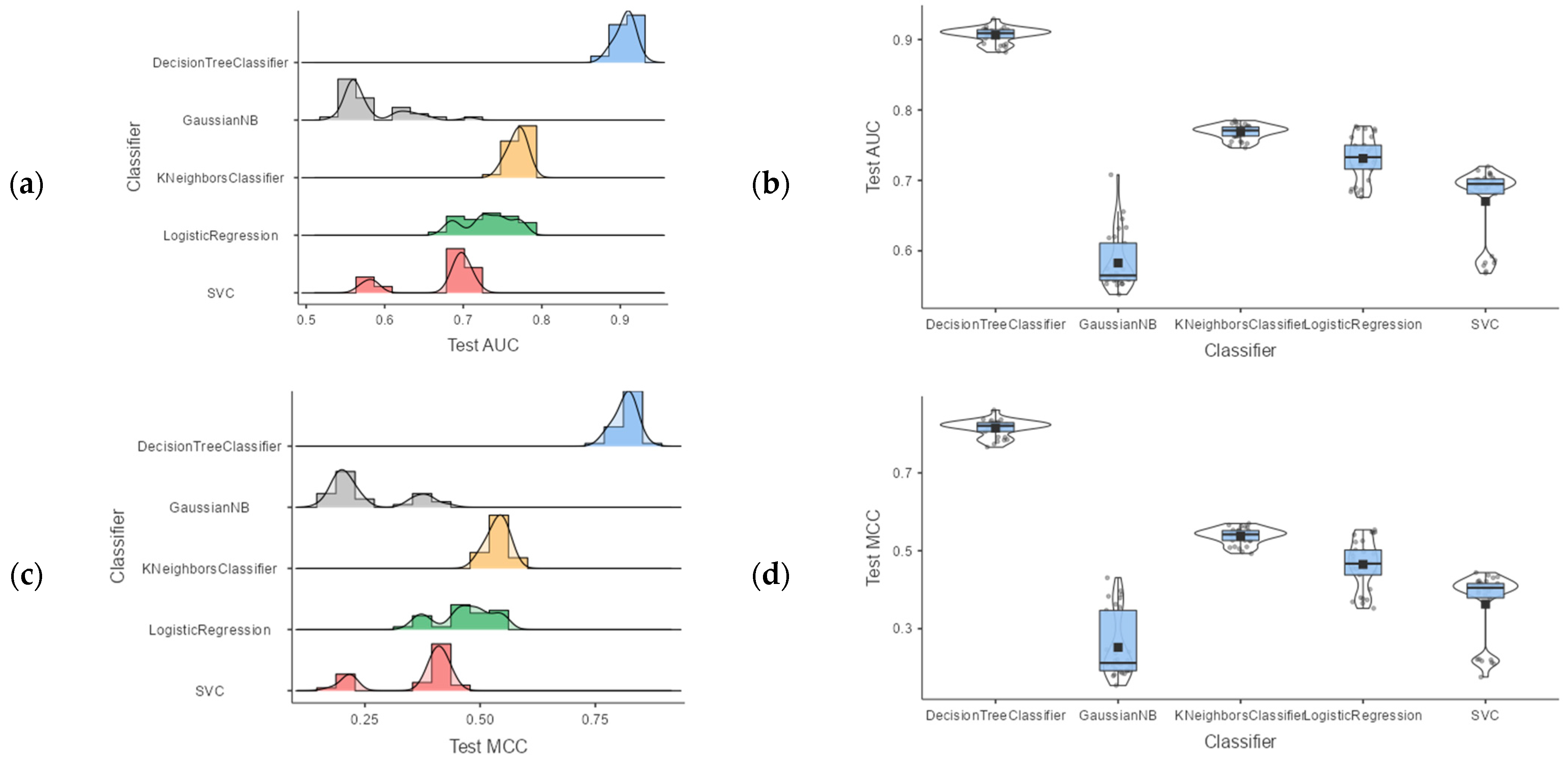
| 95% Confidence Interval | ||||||
|---|---|---|---|---|---|---|
| Classifier | Mean | Lower | Upper | Median | SD | |
| AUC | DecisionTreeClassifier | 0.906 | 0.902 | 0.910 | 0.909 | 0.0111 |
| GaussianNB | 0.583 | 0.568 | 0.597 | 0.565 | 0.0402 | |
| KNeighborsClassifier | 0.768 | 0.765 | 0.772 | 0.771 | 0.0103 | |
| LogisticRegression | 0.731 | 0.720 | 0.742 | 0.733 | 0.0311 | |
| SVC | 0.670 | 0.651 | 0.689 | 0.695 | 0.0524 | |
| MCC | DecisionTreeClassifier | 0.815 | 0.807 | 0.823 | 0.821 | 0.0217 |
| GaussianNB | 0.252 | 0.222 | 0.283 | 0.212 | 0.0838 | |
| KNeighborsClassifier | 0.537 | 0.530 | 0.545 | 0.542 | 0.0208 | |
| LogisticRegression | 0.465 | 0.443 | 0.488 | 0.467 | 0.0620 | |
| SVC | 0.363 | 0.331 | 0.395 | 0.405 | 0.0886 | |
Publisher’s Note: MDPI stays neutral with regard to jurisdictional claims in published maps and institutional affiliations. |
© 2022 by the authors. Licensee MDPI, Basel, Switzerland. This article is an open access article distributed under the terms and conditions of the Creative Commons Attribution (CC BY) license (https://creativecommons.org/licenses/by/4.0/).
Share and Cite
Pitoglou, S.; Filntisi, A.; Anastasiou, A.; Matsopoulos, G.K.; Koutsouris, D. Exploring the Utility of Anonymized EHR Datasets in Machine Learning Experiments in the Context of the MODELHealth Project. Appl. Sci. 2022, 12, 5942. https://doi.org/10.3390/app12125942
Pitoglou S, Filntisi A, Anastasiou A, Matsopoulos GK, Koutsouris D. Exploring the Utility of Anonymized EHR Datasets in Machine Learning Experiments in the Context of the MODELHealth Project. Applied Sciences. 2022; 12(12):5942. https://doi.org/10.3390/app12125942
Chicago/Turabian StylePitoglou, Stavros, Arianna Filntisi, Athanasios Anastasiou, George K. Matsopoulos, and Dimitrios Koutsouris. 2022. "Exploring the Utility of Anonymized EHR Datasets in Machine Learning Experiments in the Context of the MODELHealth Project" Applied Sciences 12, no. 12: 5942. https://doi.org/10.3390/app12125942